Multispectral Inversion of Citrus Multi-Slope Evapotranspiration by UAV Based on Modified RSEB Model

Abstract

Evaptotranspiration (ET_c) is a crucial link in the farmland water cycle process. To accurately obtain the citrus ET_c in different slope positions, the METRIC, RSEB, and FAO Penman–Monteith (P-M) models were constructed based on unmanned aerial vehicle (UAV) multispectral images to invert the ET_c values. The ET_c of citrus calculated by the P-M model was used as a reference standard, and the accuracy of the ET_c inversion was evaluated by the METRIC model and the RSEB model. The results showed that the R², RMSE, and SE of the METRIC model and the RSEB model were 0.396 and 0.486, 4.940 and 3.010, and 4.570 and 2.090, respectively, indicating a higher accuracy of the RSEB model for inverting the ET_c values. Furthermore, the accuracy of the RSEB model could be improved by introducing the optimal correction coefficient (after correction: RMSE = 1.470, SE = 0.003). Based on the modified RSEB model, the ET_c values of the citrus in different slope positions were obtained. We also found that the middle slope ET_c > the top slope ET_c > the bottom slope ET_c, indicating that the slope position indeed affected the citrus ET_c. This research provides a favorable framework for the ET_c inversion, and the results are of theoretical and practical importance to realize crop water conservation.

1. Introduction

Evapotranspiration (ET_c) is a crucial component of the hydrological cycle and water resource management and plays a key role in the exchange of material and energy within the soil–crop–atmosphere system [1,2]. ET_c serves as an important indicator that reflects the water consumption of crops, and an accurate estimation of ET_c can optimize irrigation systems and improve water resource utilization efficiency [3], which is of great significance to the development of agriculture in China. Historically and spatially, ET_c was estimated using hydrological principles [4]. In the early 17th century, Dalton proposed a model for calculating water surface ET_c from the saturated state of water vapor pressure, which formed the basis of ET_c theory [5].

In recent years, satellite remote sensing technology has been increasingly utilized for the estimation of ET_c on a large-scale regional or global level due to its wide monitoring scale. Researchers and scholars demonstrated that remote sensing energy balance models using satellite data, such as the one proposed by Peng et al. [6], could be effective for estimating ET_c. However, satellite remote sensing has limitations such as low surface resolution, susceptibility to atmospheric factors, and long revisit periods [7,8]. In contrast, UAV remote sensing has advantages such as mobility, flexibility, portability, and low cost, and is able to obtain high spatial and temporal resolution data in small- and medium-scale areas, effectively addressing many issues associated with satellite remote sensing [9,10]. UAV technology for monitoring soil and vegetation information is characterized by its fast, macroscopic, and convenient capabilities. It has been widely applied in agriculture [11]. Therefore, based on UAV remote sensing technology, ET_c models can be constructed for farmland. Hoffmann et al. [12] applied UAVs to obtain high-resolution surface temperatures for the TSEB and DTD algorithms to calculate surface evapotranspiration.

However, most existing remote sensing ET_c models were based on satellite data, and there is a need for more in-depth research on models based on UAV data [13,14]. Remote sensing ET_c models can be classified into mechanistic models, empirical regression models, and spatial feature method models. Among these, mechanistic models have been the most widely used, with single-source models, such as the SEBAL model, the S-SEBI model, and the METRIC model [15,16,17], being commonly utilized. The METRIC model, proposed by Allen et al. [18], has been widely used in many related fields due to its good fit with satellite data and relatively accurate estimation of ET_c. In contrast, multi-source models consider the effects of soil and vegetation on ET_c separately and were shown to provide better results in areas with heterogeneous vegetation cover and varying surface environments [19]. Typical multi-source models included the SHUTTLEWORTH model, RSEB model, and TSM model [20,21,22]. The RSEB model is an energy balance model designed for remote sensing and was shown to be suitable for estimating ET_c in areas with an inhomogeneous vegetation distribution by Samani et al. [23]. Ortega-Farías et al. [24] used the RSEB model to estimate the evapotranspiration in Brazilian olive groves.

Citrus is considered one of the most essential commercial fruits in the global market, where the production of citrus increased substantially from 25.1 Mt to 158.5 Mt worldwide from 1961 to 2020 [25]. China is the world’s largest citrus producer, accounting for 31% of the global citrus planting area and 25% of the global citrus production [26]. In the western Hubei region, citrus is the fruit tree with the largest planting area and the most important economic status, and the citrus industry has become one of the pillar industries of rural economic development in this region [25]. However, there were limited studies on citrus multi-slope ET_c based on UAV multispectral remote sensing data combined with the RSEB model. Therefore, this study focused on citrus in Yichang City, utilizing a UAV remote sensing platform equipped with a multispectral camera to carry out the ET_c inversion of multi-slope Newhall navel oranges in an experimental orchard. This study aimed to use the FAO Penman–Monteith (P-M) model for calculating citrus ET_c as a criterion and construct a modified RSEB model with a high accuracy to achieve the fast, efficient, and accurate ET_c inversion of different slopes in a citrus orchard. The research results of this study will provide technical support and a reference basis for the estimation of ET_c in different terrains at the regional scale using UAV remote sensing images.

2. Materials and Methods

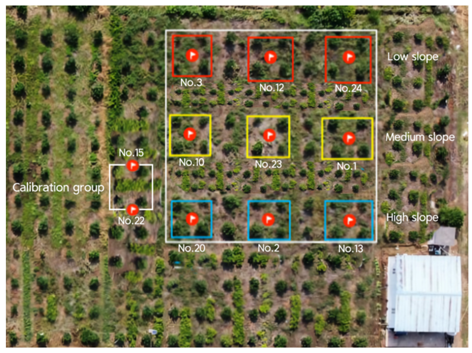
2.1. Overview of the Experimental Area

This experiment was conducted at the Zhijiang experimental field of the Yichang Institute of Agricultural Science, Hubei Province, at latitude 30°58.26′ N and longitude 111°79.05′ E, as shown in Figure 1. The fruit tree variety studied was the Newhall navel orange, with the fruit trees spaced 4 m × 4 m apart within the 28 m × 28 m experimental orchard. The growth of the fruit trees was generally consistent. The lowest point of the experimental orchard was 89 m above sea level, while the highest point was at 92 m above sea level, resulting in a height difference of approximately 3 m. The region’s climate is classified as subtropical monsoon humid, characterized by four distinct seasons, the simultaneous presence of water and heat, an annual frost-free period of 271 days, an average annual rainfall of 1019 mm, and annual sunshine hours of 1895.7 h. The average annual temperature is 16.9 °C, with an annual extreme maximum temperature of 39.3 °C, and an annual extreme minimum temperature of −14.8 °C. This climate is suitable for citrus planting and growth.

2.2. Experimental Design

From July 2022 to November 2022, the experiment involving the UAV inversion of ET_c for citrus crops in the field was divided into 10 areas, consisting of 1 calibration group and 9 experimental groups. The average area of each section was 16 m², and the growth of citrus trees in each area was generally uniform, as shown in Figure 2. All factors such as the irrigation amount, fertilizer application, fertilizer type, dosing amount, and dosing type were consistently maintained.

To mitigate any border influence, the experimental area was positioned in the center of the citrus orchard, with two longitudinally aligned spacing areas of 8 m between each experimental group and four spacing rows between the three groups. This layout aimed to minimize the impact of measurement data between each experimental group. Three categories for primary planting slopes of citrus—top slope, medium slope, and bottom slope—were established. The difference in planting height between the top slope and bottom slope was approximately 3 m, with a 15° slope. Three replicates were instituted for each treatment to ensure result accuracy.

2.3. Experimental Observation Data

2.3.1. UAV Multispectral Data

The multispectral images were captured using a drone (DJI Elf 4, DJI, Shenzhen, China) equipped with a multispectral camera. These data were used for the METRIC model and RSEB model, with the collected images having a resolution of 1280 × 720 pixels and a wavelength range of 434~886 nm. The experiment was primarily conducted from September to November, which are the two key reproductive periods of citrus: the fruit expansion period and the period of color change and sugar increase [27,28]. The data collection took place during sunny, windless (breeze) weather around midday, with data being collected 8~10 times per month. The drone flew at an altitude of 70 m, at a speed of 3 m/s, along 9 flight routes, and for a duration of 15 min.

Following the acquisition of the complete raw multispectral orthoimagery of the citrus ochard, data preprocessing was carried out. The DJI mapping software (DJI Terra 3.0.0) was used for the atmospheric calibration, calibration, and data stitching to obtain the full spectral image data for the day (Figure 3a). Subsequently, ENVI software (ENVI 5.3) was utilized to process the multispectral digital information (Figure 3b–d), extract the reflectance of the two bands of the spectrum, and calculate the vegetation index (Figure 3e).

2.3.2. Meteorological Data

The meteorological data were from a small meteorological monitoring station, which was located approximately 25 m from the experimental area (PH-1, Hubei Zechuan Technology Corporation, Yichang, China). These data were used for the FAO Penman–Monteith method, METRIC model, and RSEB model.

2.4. Mathematical Modeling

2.4.1. FAO Penman–Monteith Method

ET₀ was calculated by the FAO Penman–Monteith formula [29,30]:

$$E{T}_0=\frac{0.408\Delta \left(R_n-G\right)+\gamma \frac{900}{T+273}{U}_2\left(e_s-e_a\right)}{\Delta +\gamma (1+0.34U_2)}$$

(1)

ET_C was calculated by the crop coefficient method [31]:

$$E{T}_C=K_{C}E{T}_0$$

(2)

where ET₀ is the reference daily evapotranspiration (mm/day); R_n is the net radiation (MJ/m²); G is the soil heat flux (MJ/m²·day); T is the average air temperature at a height of 2 m (°C); U₂ is the wind speed at a height of two meters (m/s); e_s is the saturated water pressure (kPa); e_a is the actual water pressure (kPa); e_s − e_a is the difference in the saturated water and air pressure (kPa); Δ is the slope of the saturated water pressure curve (kPa/°C); γ is the humidity constant (kPa/°C); Kc is the crop coefficient, where the experimental crop was citrus with a surface weed cover, a tree height between 1.3 and 1.8 m, and canopy cover of 20% of the value taken so that the coefficient value was taken as follows: Kc = 0.85 [32,33].

2.4.2. METRIC Modeling Approach

The METRIC model derives the latent heat flux LE by calculating the relevant components of the surface energy balance, and thus, estimates ET_c using the following formula [34]:

$$R_n-G-H=LE=ET\cdot \frac{\delta {\rho }_w}{3600}$$

(3)

where R_n is the net radiative flux (W/m²); G is the soil heat flux (W/m²); H is the sensible heat flux (W/m²); LE is the latent heat flux (W/m²); ET is the hourly evapotranspiration (mm/h); ρ_w is the density of water (kg/m³), where the density of water at room temperature is 1.0 × 10³ kg/m³; δ is the latent heat of evaporation (J/kg), i.e., the heat absorbed by evaporation of 1 kg of water; and 3600 is in seconds.

Multispectral remote sensing to obtain a large amount of data and high spectral resolution can be effective to show the characteristics of the features. The METRIC model formulas for estimating the soil heat flux and sensible heat flux are as follows [35]:

$$G=\frac{T_S-273.15}{\alpha }\left(0.0038\alpha +0.0074{\alpha }^2\right)\left(1-0.98NDV{I}^4\right)R_n$$

(4)

$$H=\rho C_{pair}\frac{\Delta T}{r_{ah}}$$

(5)

where T_s is the surface temperature (K); ρ is the air density (kg/m³); C_pair is the constant pressure specific heat of air (J/(kg × k)); ΔT is the difference in air temperature (K); and r_ah is the aerodynamic impedance of heat transfer (s/m).

2.4.3. RSEB Modeling Approach

The RSEB model can be used to estimate latent heat fluxes in areas where the surface was partially covered by vegetation. It is a two-layer model, which can more accurately characterize the surface fluxes in areas where the vegetation is not uniformly distributed than in a single-layer model. Like the METRIC model, the RSEB model was used to estimate the instantaneous ET_c from the surface by calculating the latent heat flux LE from the relevant components of the energy balance of the surface and then estimating the ET_c, first by calculating R_n [24]:

$$R_n=f_r\times R_{nc}+\left(1-f_r\right)\times R_{ns}$$

(6)

where R_n is the canopy net radiation component (W/m²); R_ns is the soil net radiation component (W/m²); and f_r is the minimum cover, which is obtained by dividing the vegetation and obtaining the ratio of vegetation area to total area.

Due to the large differences in albedo and surface temperature between the soil and canopy, the net radiative components of the two were obtained separately and summed up to obtain the total net radiative flux based on the ratio of the two. The instantaneous values of R_nc and R_ns were calculated by an equilibrium model of longwave and shortwave radiation at the soil surface and canopy [24]:

$$R_{nc}=\left(1-{\alpha }_c\right)\times R_{se}+L_{in}-L_{outc}-\left(1-{\epsilon }_c\right)\times L_{in}$$

(7)

$$R_{ns}=\left(1-{\alpha }_s\right)\times R_{se}+L_{in}-L_{outs}-\left(1-{\epsilon }_s\right)\times L_{in}$$

(8)

where α_s is the soil albedo; α_c is the canopy albedo; R_se is the downward solar shortwave radiation (W/m²); L_in is the instantaneous incoming longwave radiation (W/m²); L_outs is the instantaneous outgoing longwave radiation from the soil (W/m²); L_outc is the instantaneous outgoing longwave radiation from the canopy (W/m²); ɛ_s is the soil surface thermal emissivity; and ɛ_c is the canopy surface thermal emissivity.

The estimation method of G that introduces multispectral data can better take into account the effect of vegetation on ET_c, and the scope of application was also wider [36]. In order to make the estimation method applicable to the field experimental environment at a higher level, Equation (4) was chosen for the calculation of G in this experiment.

Next, the sensible heat flux was calculated using the equations shown below [37]:

$$H=f_r\times H_c+\left(1-f_r\right)H_s$$

(9)

$$H_c=\frac{\rho C_{pair}\left(T_c-T_a\right)}{r_a^c-r_a^a}$$

(10)

$$H_s=\frac{\rho C_{pair}\left(T_s-T_a\right)}{r_a^s-r_a^a}$$

(11)

where H_c is the canopy sensible heat flux component (W/m²); H_s is the soil sensible heat flux component (W/m²); r_a^c is the aerodynamic impedance above the canopy (s/m); r_a^a is the aerodynamic impedance between the canopy and the reference level (s/m); r_a^s is the aerodynamic impedance between the soil and the canopy (s/m); and C_pair is the constant-pressure specific heat of the air (J/(kg × k)).

3. Results and Analysis

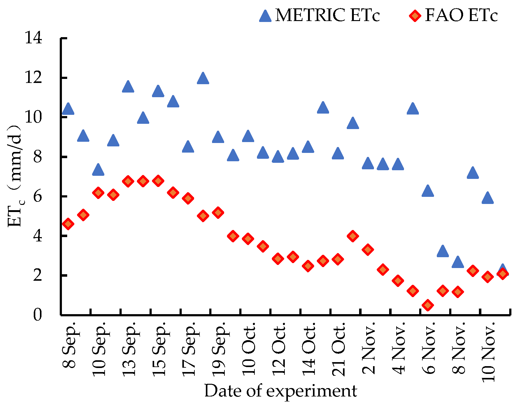
3.1. Inversion of Citrus ET_c Based on the METRIC Model

Based on the spectral data collected by UAV remote sensing, the METRIC model was constructed. Using the P-M model combined with the meteorological data, the ET_c of the Newhall navel oranges during the experimental period (fruit expansion period and color change and sugar increase period) was calculated separately, and the correlation between the two was compared to evaluate the estimation effect of the METRIC model. The results are shown in Figure 4, Figure 5 and Figure 6. The ET_c values of different slopes inverted by the METRIC model were one-way ANOVA analyzed and correlation analyzed using SPSS 23 software (IBM SPSS Statistics 23) and were multiply compared using Duncan’s test, where different lowercase letters represent significant differences in the ET_c values of different slopes at the p < 0.05 level, and the standard deviations were calculated, as shown in Figure 6.

Figure 4 depicts the ET_c change process of the Newhall navel oranges in two growth periods simulated using the METRIC model and P-M formula (average ET_c of the whole experimental area). The lowest value of ET_c estimated based on the METRIC model was 2.30 mm/d during the color change and sugar increase period, while the highest value was 11.98 mm/d during the fruit expansion period.

Figure 5 presents the results of ET_c calculated by the two methods to establish univariate linear regression model. The resulting coefficient of determination (R²) was 0.396, the root-mean-square error (RMSE) was 4.940, and the systematic error (SE) was 4.570. This indicated that using the METRIC model to calculate the ET_c of the Newhall navel orange had a larger error, and there was a significant difference in the values of the ET_c estimated by the two methods.

From the ET_c space shown in Figure 6, the average ET_c in the mid-slope treatment was the highest at 8.33 mm/d, followed by the low-slope treatment at 8.28 mm/d, and the smallest in the high-slope treatment at 8.21 mm/d. The differences were relatively small, indicating a stable state in the daily average ET_c of citrus under the three treatments. The overall trend of daily ET_c estimated by the two methods used in this study was basically the same, except for differences in some extreme values between the two growth periods of citrus.

3.2. Influence Factor Analysis of ET_c Based on METRIC Model

Based on the METRIC model, the relationship between ET_c and each influencing factor was analyzed, and the results are shown in

Table 1. Summary of each influence factor of the METRIC model.

Factor	Relevant Formula	R2	Relevance
Air velocity	y = −0.2426x + 4.4457	0.5844	Negative correlation
Temp	y = 0.6678x + 16.366	0.2338	Positive correlation
Net radiation	y = 2.1154x + 580.92	0.4371	Positive correlation
Shortwave radiation	y = 2.4274x + 704.02	0.4216	Positive correlation
Uplink longwave radiation	y = 3.3202x + 337.26	0.2324	Positive correlation
Downlink longwave radiation	y = 2.6729x + 259.51	0.2324	Positive correlation
Vegetation cover index	y = 0.0009x + 0.8027	0.0359	Positive correlation
Aerodynamic roughness	y = −0.0816x + 1.3083	0.5575	Negative correlation
Aerodynamic Impedance	y = 0.6987x + 2.5427	0.8657	Positive correlation

Note: x represents ET_c, y represents each impact factor.

. Evapotranspiration showed a high negative correlation with wind speed (R² = 0.584). Higher wind speed attenuates the energy of shortwave radiation and reduces the energy of water molecule transport, thus affecting the evapotranspiration. On the other hand, the correlation between ET_c and temperature was poor (R² = 0.234), showing a positive correlation. The appropriate wind speed for dispersing the crop-saturated air had a greater effect on ET_c than the temperature enhancement.

When comparing the relationship between the four types of radiation and the amount of ET_c, the net radiation (R_n) and shortwave radiation (R_s) had the greatest impacts on ET_c (R² = 0.437 and 0.422, respectively), whereas upward longwave radiation (R_L↑) and downward longwave radiation (R_L↓) had relatively smaller impacts (R² = 0.232). This was attributed to the different roles of each type of radiation. R_n is the combination of two types of radiation (R_ns and R_nl). R_L↑ represents the energy emitted to the atmosphere by the Earth’s surface after absorbing shortwave radiation, which has a relatively small effect on evaporation. Conversely, R_L↓ represents the energy emitted by the atmosphere that is received again by the Earth’s surface; although it also directly provides energy to the ET_c process, it has little effect due to its instability and the relatively small energy provided.

Next, the correlations of indirectly influenced factors, such as the vegetation index (NDVI), aerodynamic roughness (z_o), and aerodynamic impedance (r_ah), were analyzed. As shown in Table 1, the correlation between NDVI and ET_c was extremely low (R² = 0.036). In contrast, the correlation of z_o and r_ah with ET_c was highly significant (R² = 0.558 and 0.866, respectively). z_o exhibited a negative correlation with ET_c, while r_ah showed a positive correlation with ET_c. A larger r_ah makes it more difficult for heat to rise to the atmosphere above the canopy, causing more heat to remain at the surface below the canopy and resulting in increased ET_c.

Unlike the P-M formula, the METRIC model was constructed by incorporating additional parameters related to the wind speed, such as z_o and r_ah, the results are shown in

Table 2. Comparison table of the two models.

	Factor	Air Velocity	Temp	Net Radiation	Vapor Pressure Difference
Model (R2)
P-M formula		0.3102	0.8017	0.5367	0.8272
METRIC model		0.5844	0.2338	0.4371	0.3388

. This led to an increased sensitivity to the wind speed factor and reduced sensitivity to the temperature. While the formula does not explicitly describe the water vapor pressure difference, the saturated water vapor pressure is a function of temperature. Therefore, a linear fit of the water vapor pressure difference to the METRIC model revealed a low correlation (R² = 0.339).

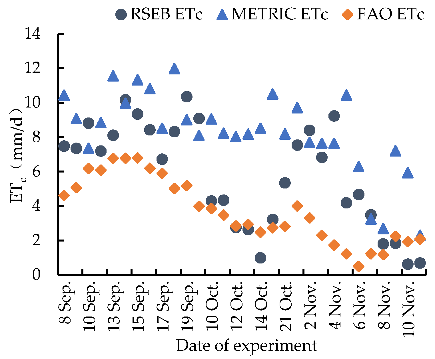
3.3. Inversion of Citrus ET_c Based on the RSEB Model

Based on the UAV spectral remote sensing data, the RSEB model was constructed to estimate the ET_c of the citrus orchard. The effectiveness of the RSEB model was assessed by comparing it with the ET_c data calculated by the P-M model. The optimal model was then derived by comparing it with the METRIC model. The results are shown in Figure 7, Figure 8, Figure 9 and Figure 10. The ET_c values of different slopes inverted by the RSEB model were one-way ANOVA analyzed and correlation analyzed using SPSS 23 software and were multiply compared using Duncan’s test, where different lowercase letters represent significant differences in the ET_c of different slopes at the p < 0.05 level, and the standard deviations were calculated, as shown in Figure 10.

Figure 7 illustrates the changes in ET_c of the Newhall navel oranges during the two growth periods, as estimated by the RSEB model and P-M formula. The lowest value of ET_c based on the RSEB model was 0.63 mm/d at the end of the color change and sugar increase period (close to the fruit-picking period), with the highest value being 10.35 mm/d during the fruit expansion period.

In Figure 8, the univariate linear regression model for the ET_c results calculated by the two methods is presented, yielding a simulation effect of the two methods (R² = 0.486) with a regression equation of y = 0.4357x + 1.1836. The root-mean-square error (RMSE) was 3.010, and the systematic error (SE) was 2.090.

Figure 9 indicates a clear difference in the values of the ET_c estimated by the three methods. The values estimated by the METRIC model were much larger than those estimated by the remaining two methods, while the values estimated by the RSEB model were closer to the results calculated by the P-M formula. Consequently, the RSEB model was a better choice than the METRIC model for estimating the ET_c in citrus zones using UAV multispectral remote sensing.

In Figure 10, the average ET_c of the different experimental treatments was the highest at the mid-slope position (5.82 mm/d), followed by the high-slope position (5.81 mm/d) and lowest at the low-slope position (5.78 mm/d). Overall, the mean ET_c was relatively stable across the three different treatments, which was consistent with the conclusion of the METRIC model. However, the RSEB model exhibited a more pronounced response to the influence of the surrounding environment, reflecting a more realistic estimation of the mean ET_c among the different treatments of citrus crops. During the two growth periods of the experiment, the values of the daily ET_c estimated by the RSEB model and P-M formula were very close to each other. Most of the time, the ET_c values estimated by the P-M formula were smaller than those estimated by the RSEB model. However, at the end of the color change and sugar increase period and close to the fruit picking period, the values alternated. This could be attributed to the decrease in the water dependence of the mature citrus fruit and the temperature decrease had a great impact on the estimation of the RSEB model. Fitting ET_c using the two models and the P-M formula, respectively, where the RSEB model and the P-M formula fitted ET_c with higher correlation. The results are shown in

Table 3. Fitting ET_c using the two models and the P-M formula.

Model	Regression Equation	R2	RMSE	SE
RSEB model	y = 0.4357x + 1.1836	0.486	3.010	2.090
METRIC model	y = 0.4996x − 0.4241	0.396	4.940	4.570

.

3.4. Influence Factor Analysis of ET_c Based on the RSEB Model

The effectiveness of the impact factors was first analyzed in terms of the basic meteorological factors, which were used to explore the reason why the RSEB model fit the P-M formula better than the METRIC model. The basic meteorological factors included temperature, wind speed, and radiation. Unlike the P-M formula and the METRIC model, the RSEB model had a very detailed classification of temperature, which was divided into the atmospheric temperature T_a (the same as that used in the P-M formula), surface temperature T_s (the same as that used in the METRIC model), and canopy temperature T_c, which was unique to the RSEB model. The results of fitting the basic meteorological factors were as follows: The R² for wind speed was 0.282. The linear relationship was negatively correlated, which was close to the results of the previous subsection, but the wind speed factor had a much smaller effect on the RSEB model than on the METRIC model.

Comparing the three temperature and ET_c fits, T_a, T_s, and T_c had different fits (the R² values were 0.770, 0.258, and 0.348, respectively), with T_a having the highest effect on the ET_c value, which was close to the P-M formula. This indicated that the temperature factor had the same effect on the RSEB model as that of the P-M formula. Comparing the three kinds of radiation and ET_c values, the fit of emitted longwave radiation was much better than that of soil-emitted longwave radiation and canopy-emitted longwave radiation (the R² values were 0.756, 0.260, and 0.355, respectively), the results are shown in

Table 4. Summary of factors associated with the RSEB model.

Factor	Relevant Formula	R2	Relevance
Air velocity	y = −0.2476x + 4.452	0.282	Negative correlation
Air temperature	y = 2.2004x + 9.8376	0.7695	Positive correlation
Surface temperature	y = 0.5525x + 18.689	0.2582	Positive correlation
Canopy temperature	y = 1.0875x + 290.46	0.3475	Positive correlation
Net radiation	y = 1.129x + 717.57	0.1471	Positive correlation
Radiate longwave radiation	y = 9.8418x + 272.94	0.7561	Positive correlation
Longwave radiation from the soil	y = 2.4396x + 307.68	0.26	Positive correlation
Longwave radiation from the canopy	y = 6.2044x + 382.73	0.3546	Positive correlation

Note: x represents ET_c, y represents each impact factor.

. The fit of the ET_c values of the P-M formula to the emitted longwave radiation values yielded a better fit (R² = 0.562), which indicated that radiation was also a major influence factor of the P-M formula and the RSEB model. The effect of the temperature factor on the RSEB model was consistent with that of the P-M formula and both were positively correlated in the same way.

The fits of the two most important factors affecting ET_c, H sensible heat flux and G soil heat flux, were analyzed. Through

Table 5. Summary of key factors of variation.

Model	Sensible Heat Flux H	Soil Heat Flux G
RSEB model	0.9992	0.3936
P-M formula	0.4928	0.8511

, we found that the RSEB model fitted well to the H sensible heat flux (R² = 0.999) and less well to the G soil heat flux (R² = 0.394). This finding was completely opposite to the P-M formula, which showed a fit to H of R² = 0.493 and fit to G of R² = 0.851. Both fits were not optimal, and there was some error in the estimates.

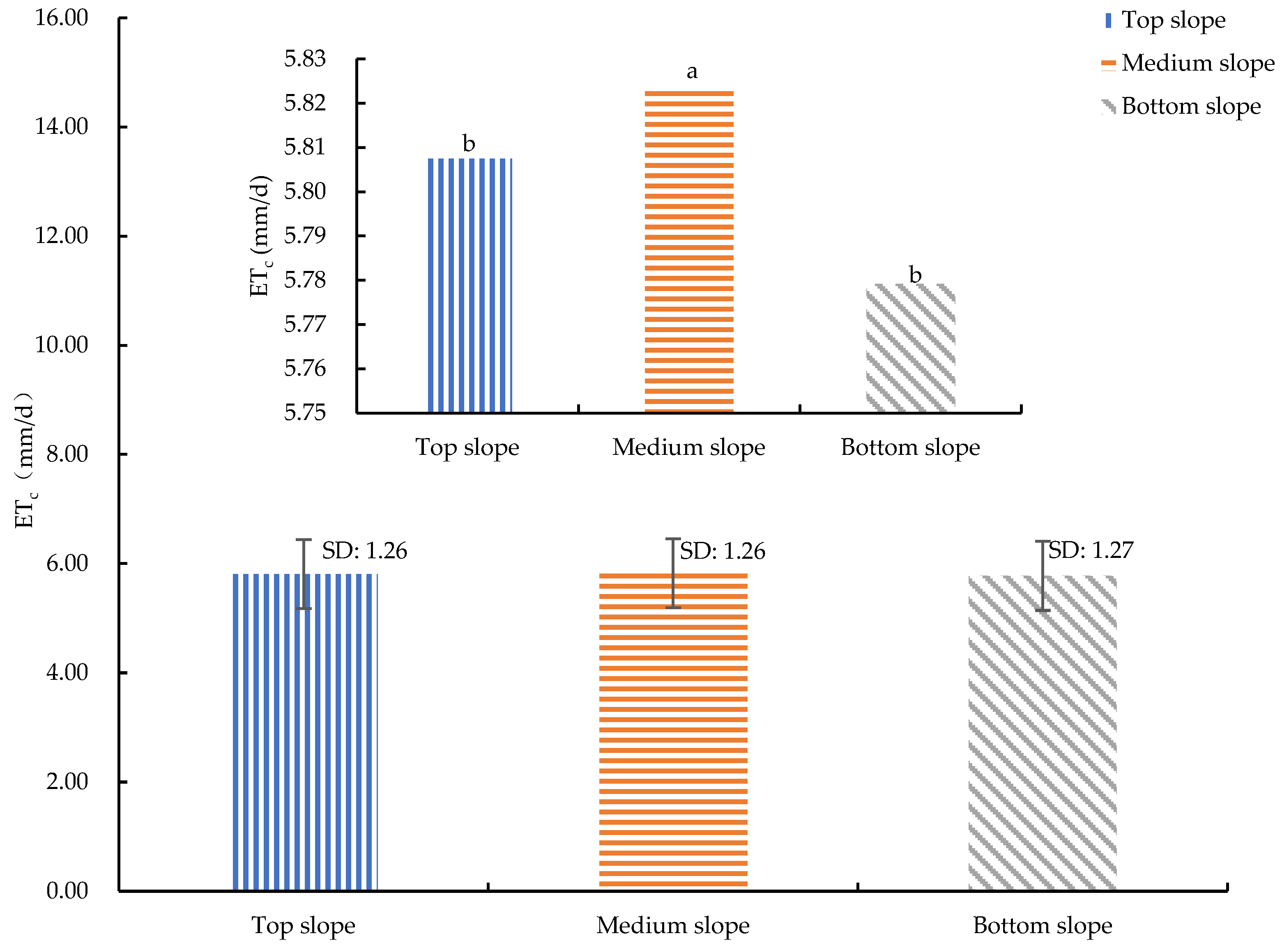
3.5. Inversion of ETc from Citrus Orchard

The RSEB model, which yielded higher results in the three precision validations, was chosen as the primary model for ET_c in citrus zones. However, the precision was not satisfactory based on the evaluation results of the three precision validation indicators. Therefore, the RSEB model was revised to ensure that the inversion results were more reliable and accurate compared with the original. The specific revisions are shown in

Table 6. Accuracy verification index table of different correction models.

Correction Model	R2	RMSE	SE
RSEB	0.486	3.010	2.090
0.7 RSEB	0.486	1.590	0.350
0.65 RSEB	0.486	1.490	0.060
0.6 RSEB	0.486	1.450	−0.230
0.64 RSEB	0.486	1.470	0.003
0.63 RSEB	0.486	1.460	−0.050

.

The results in Table 6 represent the ET_c results calculated by RSEB multiplied by several conversion factors of 0.70, 0.65, 0.64, 0.63, and 0.60 before comparing them with the standard values. Where R² represents no change in the degree of fit, the RMSE and SE values were significantly decreased, indicating that the corrected fit was improved. Since there was not much difference in the RMSE after the correction of several conversion factors of 0.65, 0.64, 0.63, 0.60, the final correction factor of 0.64 was chosen since it had the smallest systematic error (SE).

Using the modified RSEB model (0.64 RSEB) in a time series, the four trees were divided into a group of nine sets of three different treatments, and the results of the inversion of ET_c from citrus fields in the top slope treatment (No. 13, No. 2, No. 20), the medium slope treatment (No. 1, No. 23, No. 10), and the bottom slope treatment (No. 24, No. 12, and No. 3) are shown in Figure 11, Figure 12 and Figure 13.

The inversion of ET_c of citrus on different slopes was realized by using UAV multispectral remote sensing with the RSEB model and simple corrections. It was evident that the ET_c of crops under the same treatment was generally consistent and decreased with time, with some variations in specific values. Notably, the ET_c value of the medium slope treatment was 3.745 mm/d greater than that of the high-slope treatment and 3.747 mm/d greater than that of the low-slope treatment due to the vigorous growth of weeds. The average ET_c of the top slope treatment was 0.063 mm/d more than that of the bottom slope treatment, indicating that the ET_c varied greatly when there was a difference in the amount of weed cover. Conversely, the height of the slope did not significantly impact the ET_c, suggesting that the effect of weeds should be carefully considered when planting mandarin oranges in the field. Timely weeding is crucial, as excessive weeds could consume more soil water content, leading to insufficient irrigation for the mandarin oranges, and subsequently causing a decrease in fruit quality. When setting up the citrus field trial treatments, strict control over the weed coverage, height, and species is essential. The next step could involve quantifying the weed coverage, allowing for more accurate and controlled trial results.

4. Discussion

In this study, by comparing the inversion accuracy of two models, METRIC and RSEB, it was found that the RSEB model performed better. Overall, the inversion accuracy of the two models needed to be improved, which might have been due to the existence of artificial errors in the actual measurement process, and a sudden change in the weather could also make the meteorological data have errors [38], which, in turn, affected the verification accuracy of the P-M formula. In this study, only two of the more commonly used energy balance models were selected, and the accuracy of more models still needs to be subsequently verified. In addition, Liu et al. pointed out that eliminating the soil background is the key to obtaining accurate canopy spectral information [39]. Therefore, subsequent experiments should enhance access to citrus spectral data to further validate this idea. In this study, only multispectral remote sensing data were used to invert citrus evapotranspiration, and thermal infrared remote sensing fused with multispectral remote sensing will be used to further verify the inversion accuracy in the later stage.

This experiment was conducted during two critical growth periods, the fruit expansion stage and the color change and sugar increase stage, while it was crucial for guaranteeing the quality of citrus fruit and water-saving irrigation to meet the water consumption of citrus in all growth periods using precise irrigation [40], and the subsequent research will be carried out on the ET of citrus throughout the whole growth period.

In this specific experiment, the evapotranspiration was not significantly affected by the height of the slope, where the evapotranspiration was the largest in the middle slope, which may have been caused by the larger weed cover in this slope. In further citrus field experiment treatment settings, there should be strict control over the weed cover, height, and species, and thus, the next step can include a quantitative assessment of the weed cover so that the results of the experiment will be more accurate and controlled. Alternatively, research could be conducted specifically on the effects of different weed covers on citrus evapotranspiration.

5. Conclusions

(1) The ET_c of the Newhall navel oranges in the citrus orchard was estimated using the METRIC model, where the lowest values occurred during the color transition and sugar enhancement period, and the highest values occurred during the fruit expansion period. Among the different treatments, the mean ET_c was the highest in the mid-slope treatment, followed by the low-slope treatment, and lowest in the high-slope treatment. The accuracy of the ET_c estimation using the METRIC model was verified against the P-M model, with R² = 0.396, RMSE = 4.940, and systematic error (SE) = 4.570.

(2) The estimation of the ET_c of Newhall navel oranges in the citrus orchard using the RSEB model revealed the lowest value during the color transition and sugar enhancement period, and the highest value during the fruit expansion period. Among the different treatments, the mean ET_c was highest in the mid-slope treatment, followed by the high-slope treatment, and lowest in the low-slope treatment. The accuracy of the ET_c estimation using the RSEB model was verified against the P-M model, with R² = 0.486, RMSE = 3.010, and systematic error (SE) = 2.090. The RSEB model inversion was found to be better than that of the METRIC model.

(3) The optimal modification coefficient of the RSEB model was determined to be 0.64. After the modification, RMSE = 1.470, SE = 0.003, and R² remained unchanged, resulting in more accurate and reliable calculation results. Based on the corrected RSEB model for the ET_c inversion in citrus zones, the mean ET_c in the medium slope treatment was 3.745 mm/d higher than that in the high-slope treatment, and 3.747 mm/d higher than that in the low-slope treatment, with the high-slope treatment being 0.063 mm/d higher than the low-slope treatment.

In this study, by using multispectral remote sensing by UAV, constructing the RSEB model, and correcting key parameters, we could realize rapid and accurate estimation of the citrus ET_c for different slopes. This can provide theoretical and technical support for the study of the citrus water–heat cycle in farmland and the formulation of irrigation systems.

References

1. Li, J.; Li, Y.; Yin, L.; Zhao, Q. A novel composite drought index combining precipitation, temperature and evapotranspiration used for drought monitoring in the Huang-Huai-Hai Plain. Agric. Water Manag. 2024, 291, 108626. [Google Scholar] [CrossRef]
2. Huang, L.; Cai, J.; Zhang, B.; Chen, H.; Bai, L.; Wei, Z.; Peng, Z. Estimation of evapotranspiration using the crop canopy temperature at field to regional scales in large irrigation district. Agric. For. Meteorol. 2019, 269, 305–322. [Google Scholar] [CrossRef]
3. Huang, H.; Song, Y.; Fan, Z.; Xu, G.; Yuan, R.; Zhao, J. Estimation of walnut crop evapotranspiration under different micro-irrigation techniques in arid zones based on deep learning sequence models. Results Appl. Math. 2023, 20, 100412. [Google Scholar] [CrossRef]
4. Peerbhai, T.; Chetty, K.T.; Clark, D.J.; Gokool, S. Estimating evapotranspiration using earth observation data: A comparison between hydrological and energy balance modelling approaches. J. Hydrol. 2022, 613, 128347. [Google Scholar] [CrossRef]
5. Aldarabseh, S.M.; Merati, P. An experimental investigation of the potential of empirical correlations derived based on Dalton’s law and similarity theory to predict evaporation rate from still water surface. Proc. Inst. Mech. Eng. Part C J. Mech. Eng. Sci. 2022, 236, 6554–6578. [Google Scholar] [CrossRef]
6. Bai, P.; Cai, C. Calibrating a remote sensing evapotranspiration model using the Budyko framework. Agric. For. Meteorol. 2023, 342, 109757. [Google Scholar] [CrossRef]
7. Cook, K.V.; Beyer, J.E.; Xiao, X.; Hambright, K.D. Ground-based remote sensing provides alternative to satellites for monitoring cyanobacteria in small lakes. Water Res. 2023, 242, 120076. [Google Scholar] [CrossRef]
8. Qin, L.; Yan, C.; Yu, L.; Chai, M.; Wang, B.; Hayat, M.; Qiu, G.Y. High-resolution spatio-temporal characteristics of urban evapotranspiration measured by unmanned aerial vehicle and infrared remote sensing. Build. Environ. 2022, 222, 109389. [Google Scholar] [CrossRef]
9. Pajares, G. Overview and current status of remote sensing applications based on unmanned aerial vehicles (UAVs). Photogramm. Eng. Remote Sens. 2015, 81, 281–330. [Google Scholar] [CrossRef]
10. Kieu, H.T.; Pak, H.Y.; Trinh, H.L.; Pang, D.S.C.; Khoo, E.; Law, A.W.K. UAV-based remote sensing of turbidity in coastal environment for regulatory monitoring and assessment. Mar. Pollut. Bull. 2023, 196, 115482. [Google Scholar] [CrossRef]
11. Matese, A.; Toscano, P.; Di Gennaro, S.F.; Genesio, L.; Vaccari, F.P.; Primicerio, J.; Gioli, B. Intercomparison of UAV, aircraft and satellite remote sensing platforms for precision viticulture. Remote Sens. 2015, 7, 2971–2990. [Google Scholar] [CrossRef]
12. Hoffmann, H.; Nieto, H.; Jensen, R.; Guzinski, R.; Zarco-Tejada, P.; Friborg, T. Estimating evaporation with thermal UAV data and two-source energy balance models. Hydrol. Earth Syst. Sci. 2016, 20, 697–713. [Google Scholar] [CrossRef]
13. Amani, S.; Shafizadeh-Moghadam, H. A review of machine learning models and influential factors for estimating evapotranspiration using remote sensing and ground-based data. Agric. Water Manag. 2023, 284, 108324. [Google Scholar] [CrossRef]
14. Wang, X.; Lei, H.; Li, J.; Huo, Z.; Zhang, Y.; Qu, Y. Estimating evapotranspiration and yield of wheat and maize croplands through a remote sensing-based model. Agric. Water Manag. 2023, 282, 108294. [Google Scholar] [CrossRef]
15. Ma, Y.; Sun, S.; Li, C.; Zhao, J.; Li, Z.; Jia, C. Estimation of regional actual evapotranspiration based on the improved SEBAL model. J. Hydrol. 2023, 619, 129283. [Google Scholar] [CrossRef]
16. Mattar, C.; Franch, B.; Sobrino, J.A.; Corbari, C.; Jiménez-Muñoz, J.C.; Olivera-Guerra, L.; Mancini, M. Impacts of the broadband albedo on actual evapotranspiration estimated by S-SEBI model over an agricultural area. Remote Sens. Environ. 2014, 147, 23–42. [Google Scholar] [CrossRef]
17. Li, H.; Li, C.; Xing, K.; Lei, Y.; Shen, Y. Surface temperature adjustment in METRIC model for monitoring crop water consumption in North China Plain. Agric. Water Manag. 2024, 291, 108654. [Google Scholar] [CrossRef]
18. Allen, R.G.; Tasumi, M.; Trezza, R. Satellite-Based Energy Balance for Mapping Evapotranspiration with Internalized Calibration (METRIC)-Model. J. Irrig. Drain. Eng. 2007, 133, 380–394. [Google Scholar] [CrossRef]
19. Ma, Y.; Liu, S.; Song, L.; Xu, Z.; Liu, Y.; Xu, T.; Zhu, Z. Estimation of daily evapotranspiration and irrigation water efficiency at a Landsat-like scale for an arid irrigation area using multi-source remote sensing data. Remote Sens. Environ. 2018, 216, 715–734. [Google Scholar] [CrossRef]
20. Qin, S.; Li, S.; Cheng, L.; Zhang, L.; Qiu, R.; Liu, P. Partitioning evapotranspiration in partially mulched interplanted croplands by improving the Shuttleworth-Wallace model. Agric. Water Manag. 2023, 276, 108040. [Google Scholar] [CrossRef]
21. Norman, J.M.; Kustas, W.P.; Humes, K.S. Source approach for estimating soil and vegetation energy fluxes in observations of directional radiometric surface temperature. Agric. For. Meteorol. 1995, 77, 263–293. [Google Scholar] [CrossRef]
22. Aryalekshmi, B.N.; Biradar, R.C.; Chandrasekar, K.; Ahamed, J.M. Analysis of various surface energy balance models for evapotranspiration estimation using satellite data. Egypt. J. Remote Sens. Space Sci. 2021, 24, 1119–1126. [Google Scholar] [CrossRef]
23. Samani, Z.; Bawazir, A.S.; Bleiweiss, M.; Skaggs, R.; Longworth, J.; Tran, V.D.; Pinon, A. Using remote sensing to evaluate the spatial variability of evapotranspiration and crop coefficient in the lower Rio Grande Valley, New Mexico. Irrig. Sci. 2009, 28, 93–100. [Google Scholar] [CrossRef]
24. Ortega-Farías, S.; Ortega-Salazar, S.; Poblete, T.; Kilic, A.; Allen, R.; Poblete-Echeverría, C.; Sepúlveda, D. Estimation of energy balance components over a drip-irrigated olive orchard using thermal and multispectral cameras placed on a helicopter-based unmanned aerial vehicle (UAV). Remote Sens. 2016, 8, 638. [Google Scholar] [CrossRef]
25. Luo, Y.; Wu, X.; Xiao, H.; Toan, N.S.; Liao, B.; Wu, X.; Hu, R. Leaching is the main pathway of nitrogen loss from a citrus orchard in Central China. Agric. Ecosyst. Environ. 2023, 356, 108559. [Google Scholar] [CrossRef]
26. Li, Y.J.; Yang, M.; Zhang, Z.Z.; Li, W.L.; Guo, C.Y.; Chen, X.P.; Zhang, Y.Q. An Ecological Research on Potential for Zero-growth of Chemical Fertilizer Use in Citrus Production in China. Ekoloji Derg. 2019, 28, 1049–1059. [Google Scholar]
27. Ma, X.; Chang, Y.; Li, F.; Yang, J.; Ye, L.; Zhou, T.; Lu, X. CsABF3-activated CsSUT1 pathway is implicated in pre-harvest water deficit inducing sucrose accumulation in citrus fruit. Hortic. Plant J. 2023, 10, 103–114. [Google Scholar] [CrossRef]
28. Chen, S.; Zhai, L.; Xie, J.; Shao, Y.; Wang, W.; Li, H.; Cen, H. Early diagnosis and mechanistic understanding of citrus Huanglongbing via sun-induced chlorophyll fluorescence. Comput. Electron. Agric. 2023, 215, 108357. [Google Scholar] [CrossRef]
29. Cunha, A.C.; Gabriel Filho, L.R.A.; Tanaka, A.A.; Goes, B.C.; Putti, F.F. Influence of the estimated global solar radiation on the reference evapotranspiration obtained through the penman-monteith fao 56 method. Agric. Water Manag. 2021, 243, 106491. [Google Scholar] [CrossRef]
30. Wu, Z.; Cui, N.; Zhao, L.; Han, L.; Hu, X.; Cai, H.; Liu, Q. Estimation of maize evapotranspiration in semi-humid regions of northern China using Penman-Monteith model and segmentally optimized Jarvis model. J. Hydrol. 2022, 607, 127483. [Google Scholar] [CrossRef]
31. Han, X.; Zhou, Q.; Zhang, B.; Che, Z.; Wei, Z.; Qiu, R.; Du, T. Real-time methods for short and medium-term evapotranspiration forecasting using dynamic crop coefficient and historical threshold. J. Hydrol. 2022, 606, 127414. [Google Scholar] [CrossRef]
32. Yagci, A.L. Estimation of instantaneous, diurnal, and daily evaporative fraction using readily available inputs in the wetlands of South Florida, United States. Int. J. Remote Sens. 2023, 44, 2115–2144. [Google Scholar] [CrossRef]
33. Jamshidi, S.; Zand-Parsa, S.; Kamgar-Haghighi, A.A.; Shahsavar, A.R.; Niyogi, D. Evapotranspiration, crop coefficients, and physiological responses of citrus trees in semi-arid climatic conditions. Agric. Water Manag. 2020, 227, 105838. [Google Scholar] [CrossRef]
34. Castellví, F.; Suvočarev, K.; Reba, M.L.; Runkle, B.R. A new free-convection form to estimate sensible heat and latent heat fluxes for unstable cases. J. Hydrol. 2020, 586, 124917. [Google Scholar] [CrossRef]
35. Yang, C.; Wu, T.; Hu, G.; Zhu, X.; Yao, J.; Li, R.; Zhang, Y. Approaches to assessing the daily average ground surface soil heat flux on a regional scale over the Qinghai-Tibet Plateau. Agric. For. Meteorol. 2023, 336, 109494. [Google Scholar] [CrossRef]
36. Kustas, W.P.; Daughtry, C.S.T. Estimation of the soil heat flux/net radiation ratio from spectral data. Agric. For. Meteorol. 1990, 49, 205–223. [Google Scholar] [CrossRef]
37. Sánchez, J.M.; López-Urrea, R.; Rubio, E.; González-Piqueras, J.; Caselles, V. Assessing crop coefficients of sunflower and canola using two-source energy balance and thermal radiometry. Agric. Water Manag. 2014, 137, 23–29. [Google Scholar] [CrossRef]
38. Ukhurebor, K.E.; Azi, S.O.; Aigbe, U.O.; Onyancha, R.B.; Emegha, J.O. Analyzing the uncertainties between reanalysis meteorological data and ground measured meteorological data. Measurement 2020, 165, 108110. [Google Scholar] [CrossRef]
39. Liu, S.; Jin, X.; Bai, Y.; Wu, W.; Cui, N.; Cheng, M.; Yin, D. UAV multispectral images for accurate estimation of the maize LAI considering the effect of soil background. Int. J. Appl. Earth Obs. Geoinf. 2023, 121, 103383. [Google Scholar] [CrossRef]
40. Segovia-Cardozo, D.A.; Franco, L.; Provenzano, G. Detecting crop water requirement indicators in irrigated agroecosystems from soil water content profiles: An application for a citrus orchard. Sci. Total Environ. 2022, 806, 150492. [Google Scholar] [CrossRef]
Figure 1. Map of the experimental area.
Water 16 01520 g001
Figure 2. Distribution of the experimental area.
Water 16 01520 g002
Figure 3. Flow chart of the spectral data extraction. Note: (a) Color composite image of the experimental area. (b) UAV multispectral image. (c) UAV multispectral image element. (d) UAV multispectral image element data statistics (the horizontal coordinate was the DN value of the image element and the vertical coordinate was the statistical value of the number of image elements). (e) Multispectral data extraction table.
Water 16 01520 g003
Figure 4. METRIC ETc and FAO ETc change process.
Water 16 01520 g004
Figure 5. Fitting of ETc calculated in METRIC and P-M.
Water 16 01520 g005
Figure 6. Average METRIC ETc for each treatment. Note: Different lowercase letters represent significant differences in ETc at the p < 0.05 level for different slopes.
Water 16 01520 g006
Figure 7. RSEB ETc and FAO ETc change process.
Water 16 01520 g007
Figure 8. Fitting of ETc calculated in RSEB and P-M.
Water 16 01520 g008
Figure 9. RSEB ETc, METRIC ETc, and FAO ETc change process.
Water 16 01520 g009
Figure 10. Average RSEB ETc for each treatment. Note: Different lowercase letters represent significant differences in ETc at the p < 0.05 level for different slopes.
Water 16 01520 g010
Figure 11. Top slope treatment.
Water 16 01520 g011
Figure 12. Middle slope treatment.
Water 16 01520 g012
Figure 13. Bottom slope treatment.
Water 16 01520 g013