Article

Utilizing Data-Driven Approaches to Forecast Fluctuations in Groundwater Table

Department of Environmental Science and Technology, University of Maryland, College Park, MD 20742, USA
*
Author to whom correspondence should be addressed.
Water 2024, 16(11), 1500; https://doi.org/10.3390/w16111500
Submission received: 9 April 2024 / Revised: 14 May 2024 / Accepted: 22 May 2024 / Published: 24 May 2024

Abstract

:
Accurate forecasting of fluctuations in groundwater table is crucial for the effective management of regional water resources. This study explores the potential of utilizing remotely sensed satellite data to predict and forecast water table variations. Specifically, two Artificial Neural Network (ANN) models were developed to simulate water table fluctuations at two distinct well sites, namely BA Ea 18 and FR Df 35 in Maryland. One model leveraged the relationship between variations in brightness temperature and water table depth, while the other model was founded on the association between changes in soil moisture and water table depth. These models were trained and validated using recorded water table depths from the aforementioned wells, brightness temperature data acquired from the Advanced Microwave Scanning Radiometer—Earth Observing System (AMSR-E), and soil moisture information generated using the Land Data Assimilation System (LDAS). All models exhibited strong performance in predicting and forecasting water table fluctuations, with root mean square errors ranging from 0.043 m to 0.047 m for a 12-month forecasting horizon. Sensitivity tests revealed that the models displayed greater sensitivity to uncertainties in water table depth compared to uncertainties in both brightness temperature and soil moisture content. This underscores the feasibility of constructing an ANN-based water table prediction model, even in cases where high-resolution remotely sensed data is unavailable. In such situations, the model’s efficacy is contingent on the compatibility of the time series trends in data, such as brightness temperature or soil moisture, with those observed at the study site.

1. Introduction

Groundwater plays a pivotal role in sustaining both the environment and human activities in Maryland, underscoring its significance in the region. As a primary source of freshwater, groundwater in Maryland supports diverse ecosystems, maintaining the flow of rivers and wetlands while nurturing vital habitats for wildlife [1]. Furthermore, it serves as a dependable source of drinking water for a substantial portion population in Maryland and the Mid-Atlantic region, with approximately 3.3 million residents relying on groundwater in Maryland alone for their domestic water needs [1,2]. In addition, stresses induced by climate change and growing populations has resulted in increased withdrawals from the confined aquifers, thus requiring timely management of this vital resource for the future sustainability of freshwater. For example, Shirmohammadi et al. (2019) reported increased freshwater withdrawals for irrigation (by about 122% since 1985) and for municipal use (by about 48% since 1985) in Maryland [3]. They showed that these heavy water withdrawals resulted in water level declines ranging from 4.3 m to about 22 m in Aquia aquifer, a major confined aquifer in the Coastal Plain of Maryland. Also, other studies emphasize the growing importance of preserving Maryland’s groundwater resources in the face of evolving challenges, such as climate change and population growth [4]. Ensuring the sustainability and quality of groundwater is paramount to mitigate water scarcity and safeguard the state’s ecosystems. Effective groundwater management strategies, informed by the latest research and proper data [5], are essential to meet the present and future water demands of residents, agriculture, and industry while protecting the environment.
Groundwater modeling has conventionally relied on conceptual or physical-based models to unravel the intricate physical processes within specific hydrological systems and decipher the complex relationships among various hydrologic variables. These models have been instrumental in enhancing our understanding of groundwater dynamics. However, a significant challenge arises in the form of a large number of parameters required during the modeling process. Acquiring and quantifying all the influential variables within a groundwater system can be a formidable and resource-intensive task and having appropriate input parameter values represents a big gap in the use of such process-based models. Moreover, certain variables exhibit nonlinear and intricate relationships, rendering them challenging to comprehend using conventional means. In response to these challenges, conventional statistical techniques, such as autoregressive (AR), autoregressive moving average (ARMA), and autoregressive integrated moving average (ARIMA), have been consistently applied to model groundwater resources [6,7,8]. ARIMA is advantageous for reducing the impact of extreme values on prediction accuracy. While linear regression methods are cost-effective, they fall short in describing complex groundwater fluctuations. Recent research often uses linear regression models as benchmarks to highlight superior alternatives [9,10,11].
Various numerical models, rooted in the Boussinesq equation, have been developed to simulate water table variations under diverse climatic and hydrological conditions [12]. Although physically based models necessitate a thorough understanding of complex input/output relationships and extensive meteorological, hydrological, and geological data for the study area [13,14], their application is hindered by the demand for substantial measurements. In addition to physically based models, alternative methods such as water balance models [15,16,17] and statistical regression models [18,19,20] have been developed and used. However, they both need large amount of input parameter values and observations to fulfill the calculation. In most field applications, the errors in model output are caused to some extent by the presence of errors or uncertainties in the input data. This therefore increases the difficulty of accomplishing the simulation in a timely manner [21].
Within the data-driven methodology for predicting groundwater levels and groundwater table, diverse techniques are accessible [22]. These encompass approaches utilizing moving averages (MA), autoregressive moving averages (ARMA), multiple linear regression (MLR) [23], artificial neural networks (ANN), support vector machines (SVMs) [24], the adaptive neurofuzzy inference system (ANFIS) approach [25], and the long short-term memory (LSTM) [26], derived from recurrent neural networks (RNN). Among these methods, artificial neural networks (ANN) have gained popularity due to their ability to account for the nonlinearity of the variables involved and showcasing the reliability of predicted results as evidenced by numerous researchers [27,28,29,30].
In contrast to numerous water quality models grounded in statistical methods that assume linear and normally distributed relationships between response and prediction parameters, artificial neural networks (ANNs) have the capability to capture the nonlinear relationships inherent in ecosystems [31,32]. However, such models are thirsty for a large relevant database that is often not available. Recent research has emphasized the application of ANN models in predicting river water quality, as highlighted in some studies [33,34,35]. Daliakopoulos et al. (2005) examined the efficacy of seven distinct artificial neural network (ANN) models with varied architectures and training algorithms for predicting groundwater levels [36]. Results of their studies indicated that the Levenberg–Marquardt algorithm proved to be the most accurate in training feed-forward ANNs. In a comparison between an ANN model and a numerical model (MODFLOW) for simulating groundwater levels in an alluvial aquifer system, the ANN model demonstrated superior predictive performance for short-term horizon forecasts, as supported by both Mohanty et al. (2013) and Shiri et al. (2013) [37,38]. Mohanty et al. (2013) used extensive database inclusive of weekly rainfall, evaporation, river stage, water level in the drain, pumping rate of the tubewells, and groundwater levels in more than 18 wells at a previous time step to predict the current groundwater levels [37]. These studies indicated that ANN modeling could provide accurate results and require little time for training and execution. However, their method required too many parameters, as listed above. As such, our study used available unique database on brightness temperatures and LDAS surface soil moisture to develop relationship between groundwater table fluctuations using ANN as a tool. This study pursues multiple objectives aimed at harnessing the potential of remotely sensed satellite data for predicting water table variations. Firstly, we aim to develop and evaluate two distinct Artificial Neural Network (ANN) models tailored to simulate water table fluctuations at two well sites: BA Ea 18 and FR Df 35 in Maryland. One model will be crafted to exploit the correlation between variations in brightness temperature and water table depth, while the second model will be based on the relationship between changes in soil moisture and water table depth. To achieve these objectives, we will meticulously train and validate the ANN models using recorded water table depths from the specified wells. Additionally, we will integrate relevant satellite-derived data, including brightness temperature information from the Advanced Microwave Scanning Radiometer—Earth Observing System (AMSR-E) and soil moisture data generated by the Land Data Assimilation System (LDAS). Our overarching goal is to enhance the predictive accuracy of water table variations, contributing to a deeper understanding of the potential applications of satellite data in hydrological modeling. Through these objectives, we aim to advance the field’s knowledge and capabilities in utilizing remote sensing for accurate water table predictions at specific well sites.

2. Materials and Methods

2.1. Data Acquisition

2.1.1. Water Table Depth Data

Maryland has three distinct physiographic regions. From west to east across the state, they are the Appalachian (Appalachian Plateau, Valley and Ridges, Blue Ridge), Piedmont, and Coastal Plain. In the Piedmont region, the formation formed mainly by unconsolidated volcanic deposits consisting mostly of sand and gravel; therefore, it is capable of providing large quantities of groundwater to the users. In 2001, there were 345 groundwater wells in Maryland that recorded the groundwater level in a variety of locations [39]. Among them, eighty wells provided groundwater level information for unconfined aquifers (provided by Wendy McPherson of USGS). Two water table wells (BA Ea 18 and FR Df 35), both in Piedmont, that recorded daily water table depths for a time span of several years were used in this study.
BA Ea 18 is located in Baltimore County, MD (39.35 N, 76.86 W) in the Woodstock Quartz Monzonite local aquifer. The land-surface elevation is 149.66 m (491 feet) above mean sea level. It recorded monthly mean water table data from October 1999 through September 2007. FR Df 35 is located in Frederick County, MD (39.42 N, 77.32 W) in the Urbana Formation local aquifer (Figure 1). The land-surface elevation is 173.74 m (570 feet) above mean sea level. It provides the monthly mean water table measurements for the period from February 2004 to September 2006. Both wells have some months without monthly mean data. The water table data at both sites were downloaded from USGS, 02/15/2008, NWISWeb (http://waterdata.usgs.gov/nwis/gw (accessed on 15 February 2008)).

2.1.2. Brightness Temperature Data

The brightness temperature retrieved from the observation of the Advanced Microwave Scanning Radiometer—Earth Observing System (AMSR-E) was used in this study. AMSR-E was launched on board the NASA EOS Aqua satellite on 4 May 2002 [39]. AMSR-E provides global passive microwave measurements of terrestrial, oceanic, and atmospheric variables. The AMSR-E Level 2A product (AE_L2A) contains brightness temperatures at six frequencies: 6.9 GHz, 10.7 GHz, 18.7 GHz, 23.8 GHz, 36.5 GHz, and 89.0 GHz. The footprint sizes of the observations are 56 km, 38 km, 24 km, 21 km, 12 km, and 5.4 km, respectively. The brightness temperature resampled at 89.0 GHz vertical (V) field with a footprint size of 5.4 km (diameter of coverage) was selected to be used for this study. The data were obtained from National Snow and Ice Data Center [40]. The monthly mean brightness temperature at the well site was computed by averaging the daily observations which fall inside a circle with a radius of 2.75 km from the well site for each month.

2.1.3. Soil Moisture Data

A high-resolution satellite remotely sensed soil moisture data with several years of coverage would be optimal for this research. However, it was not available in the study area. Therefore, instead, the soil moisture data produced by the Land Data Assimilation System (LDAS) was used.
The LDAS is a real-time, hourly, distributed, uncoupled, land surface simulation system [41]. The output of LDAS includes energy balance components, water balance components, evaporation components, surface water variables, and subsurface state variables. The LDAS produces its output at a higher spatial resolution and a longer temporal coverage which is essential in the training of ANN model. Soil moisture output from LDAS can be either hourly total soil column moisture or hourly layered soil moisture at the layers of 0–10 cm, 10–40 cm, and 40–200 cm. The soil moisture data of the North American Land Data Assimilation System (NLDAS), which is a subsystem of LDAS, was used in this study. The NLDAS runs in near real-time on a one-eighth degree grid. The spatial coverage is from 25 N to 53 N in latitude and from 125 W to 67 W in longitude. The soil moisture data were downloaded from https://ldas.gsfc.nasa.gov/nldas/mosaic (accessed on 15 February 2008). The soil moisture data at a grid location that was the closest to the well site was used for the model training at that well.

2.2. Groundwater Table

Groundwater is recharged by percolation through the unsaturated zone. The fluctuation of the water table is determined by the relative rates of recharge versus outflow. The extent of vertical variation of the water table is primarily affected by the intensity and frequency of local precipitation. A net recharge of groundwater results in a rise of the water table. Inversely, the water table will descend if there is a net discharge of groundwater. Groundwater outflow is the major cause for the lowering of the water table. Based on the water balance concept, the groundwater recharge can be derived from the soil water budget in the vadose zone. The vadose zone refers to the geologic media that lie below the surface of the earth but above the water table of the shallowest year-round aquifer [42]. The vertical water movement between the vadose zone and the unconfined saturated zone in a geologic formation is the primary mechanism that results in the water table variation. Therefore, the water table fluctuation and the soil moisture variation in the vadose zone are highly related.

2.3. Surface Brightness Temperature and Soil Moisture

The thermal microwave radiation emitted from soils strongly depends on the soil moisture content. The emission is a function of the radiometer wavelength and the distribution of the moisture in the soil [43]. Because of the large difference in dielectric constant between dry and wet soils, the microwave brightness temperature can be estimated as a function of the amount of water in the soil. Schmugge (1978) has indicated that there was a correlation of up to 0.9 between the microwave brightness temperature and the moisture in the surface layer [44]. Several algorithms have been developed and successfully retrieved soil moisture from surface brightness temperature at different spatial scales [45,46,47,48]. The relationship between surface brightness temperature and soil moisture content and the ties between soil moisture variation and the water table fluctuations were the foundation to develop an ANN model for water table fluctuation prediction.

2.4. Artificial Neural Network (ANN)

A multilayer feedforward backpropagation ANN was used in this study [49]. The mathematical basis for the back-propagation algorithm is the optimization technique known as gradient descent. The training is to minimize the total squared error of the output computed by the network. The training of a network by backpropagation method involves three stages: the feedforward of the input training pattern, the calculation and backpropagation of the associated error, and the adjustment of the weights [50]. Sigmoid function is used as the activation function in this approach. Two separate ANN models were developed for predicting monthly water table fluctuations. One is based on the relationship between surface brightness temperature variation and changes in water table depth. The other one is based on the relationship between soil moisture variation and changes in water table depth. The first model uses monthly mean AMSR-E brightness temperature and water table depth change as input. The second model uses monthly mean LDAS soil moisture and water table depth as input. The outputs of both models are predicted and forecasted water table depth.
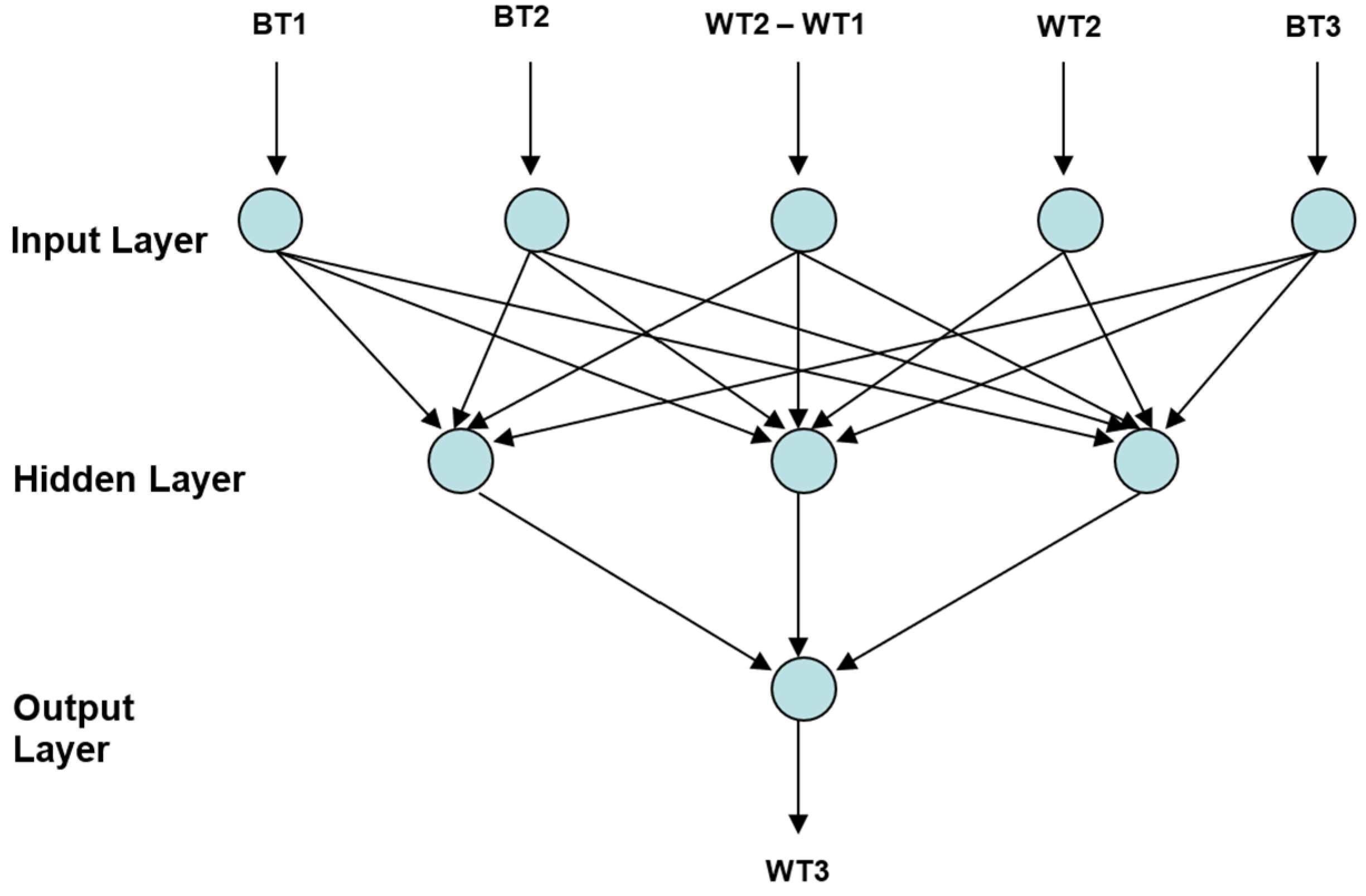
A three-layer feedforward backpropagation ANN with five input nodes in the input layer and three hidden nodes in the hidden layer was selected for building the model. The sigmoid function was used as the activation function. The monthly mean AMSR-E brightness temperature and the monthly mean water table depth at BA Ea 18 were used as input data. Figure 2 shows the structure of this three-layer ANN model, which uses previous month’s brightness temperature, current month’s brightness temperature, water table depth change in these two months, current month’s water table depth, and the subsequent month’s brightness temperature as input. These parameters are all contained in the input file. The output is the predicted subsequent month’s water table depth. Another file containing the measured water table depth for the subsequent month is used as the target file.

2.5. Statistical Analysis

We used several statistical parameters to measure the goodness of predicted groundwater table compared with the observed data and correlation between the groundwater table predictions and the input parameters used in this study. The Root Mean Square of Errors (RMSE) was used to examine the goodness of predicted/forecasted and observed groundwater tables. The RMSE may be expressed as
R M S E = i N ( P W T D i O W T D i ) N
where PWTD is the predicted water table depth, OWTD is the observed water table depth, and N is number of observations.
Also, Pearson correlation coefficient analysis with r as an indication of correlation between objective function (i.e., groundwater table) and input parameters such as the brightness temperature and the surface soil moisture. The Pearson correlation coefficient, often denoted as r, measures the strength and direction of a linear relationship between dependent and independent variables. It is commonly used in statistical analysis to compare observed data to simulation results, assessing how well the simulation corresponds to observed realities [51].
The formula for the Pearson correlation coefficient is given by
r = n x y x y n x 2 x 2 n y 2 y 2
where n is the number of data points (observations), x and y are the individual values of the observed and simulated data, respectively, Σxy, Σx, Σy, Σx², and Σy² represent the summations of the products of pairs, the values of x, the values of y, the squares of x, and the squares of y, respectively.

3. Results

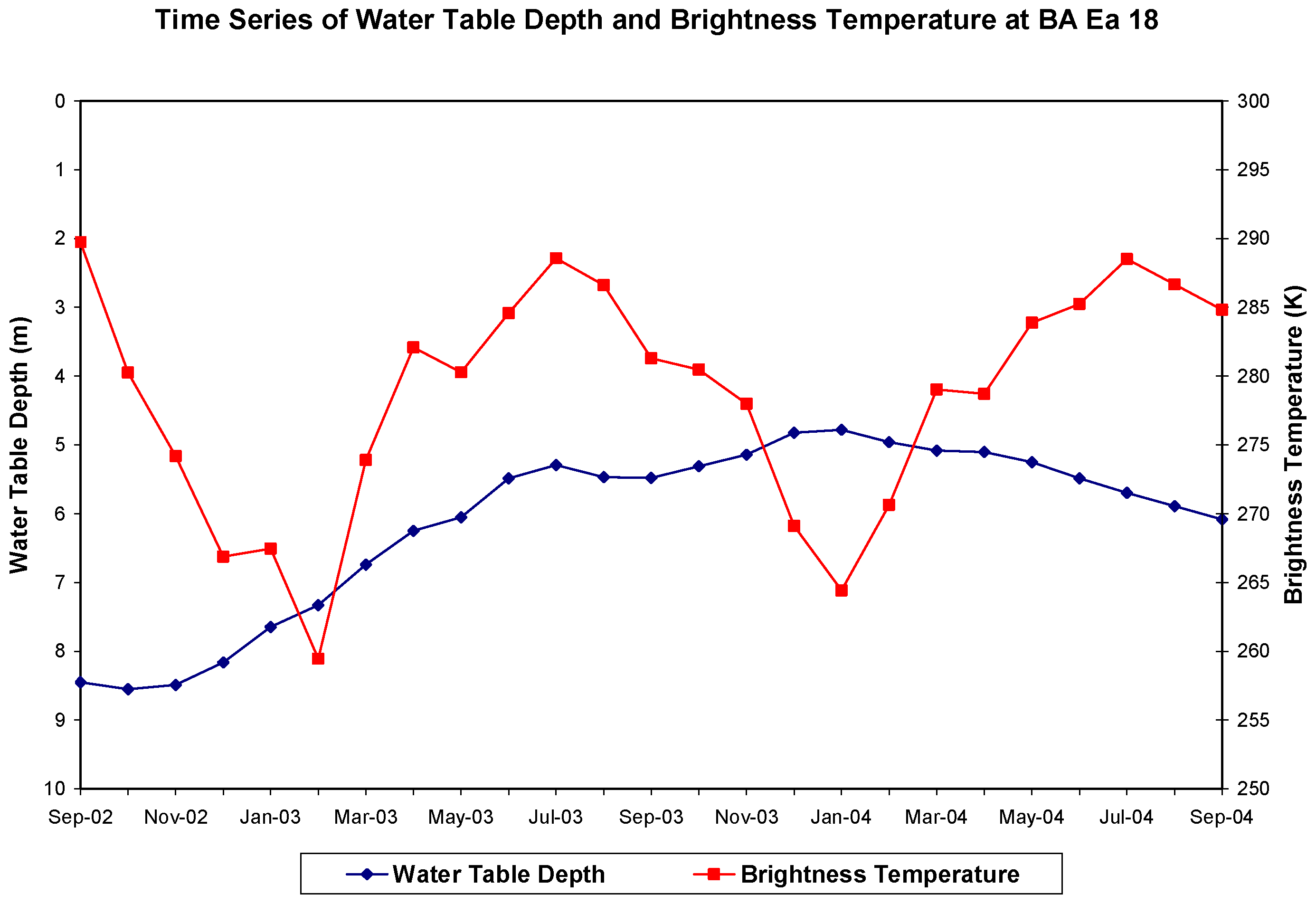
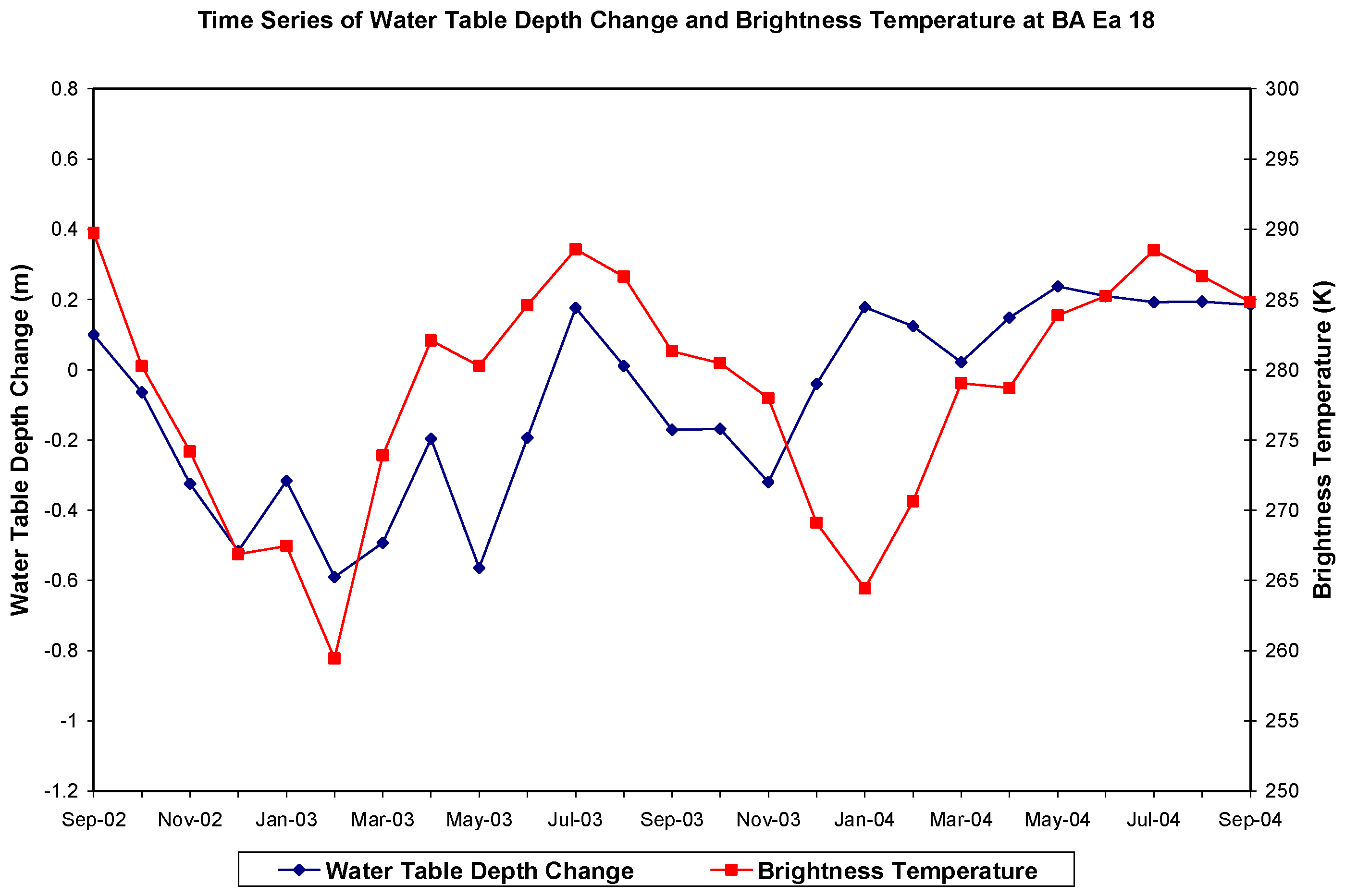
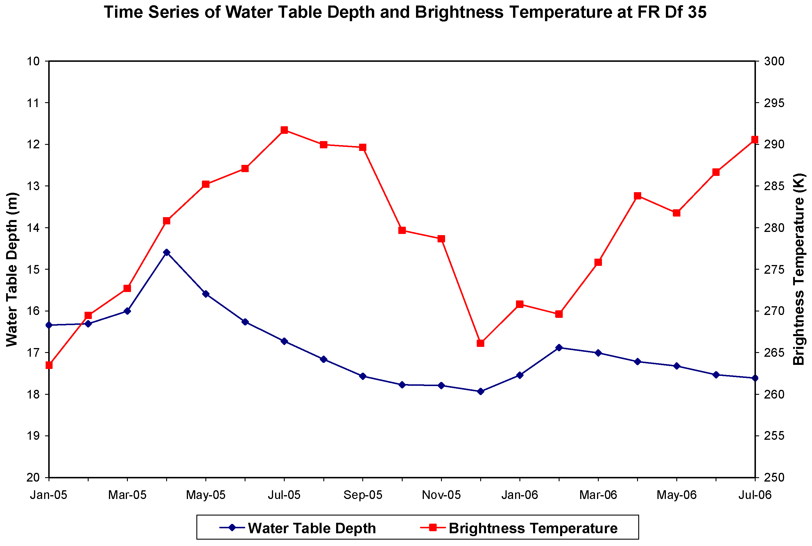
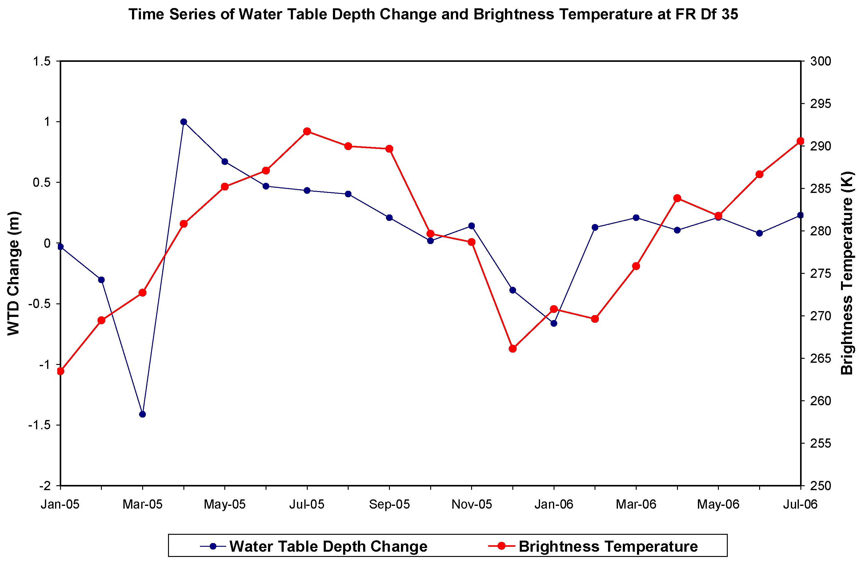
The first attempt in the development of an ANN model for water table prediction utilized monthly mean brightness temperature and monthly mean water table depth as the primary input. The time series of the groundwater table depth and that of the brightness temperature at well BA Ea 18 from September 2002 through September 2004 indicated that there was a weak negative correlation between them (r = −0.17, Figure 3). This means that as the brightness temperature increases, groundwater table declines but with a weak correlation. However, while comparing the time series of the changes in water table depth with that of the brightness temperature for the same time period, they have relatively strong positive correlation (r = 0.53) and follow similar trend as is depicted in Figure 4. Similar relationship was obtained for well site FR Df 35. The time series of water table depth and brightness temperature had a very weak positive correlation (r = 0.05, Figure 5), but their time series trend of changes in water table depth (WTD) was very similar and had a relatively strong positive correlation (r = 0.56, Figure 6). Therefore, we decided to use monthly mean water table change and monthly mean brightness temperatures as the input for the ANN model training at both well sites as a reasonable approach in this study.
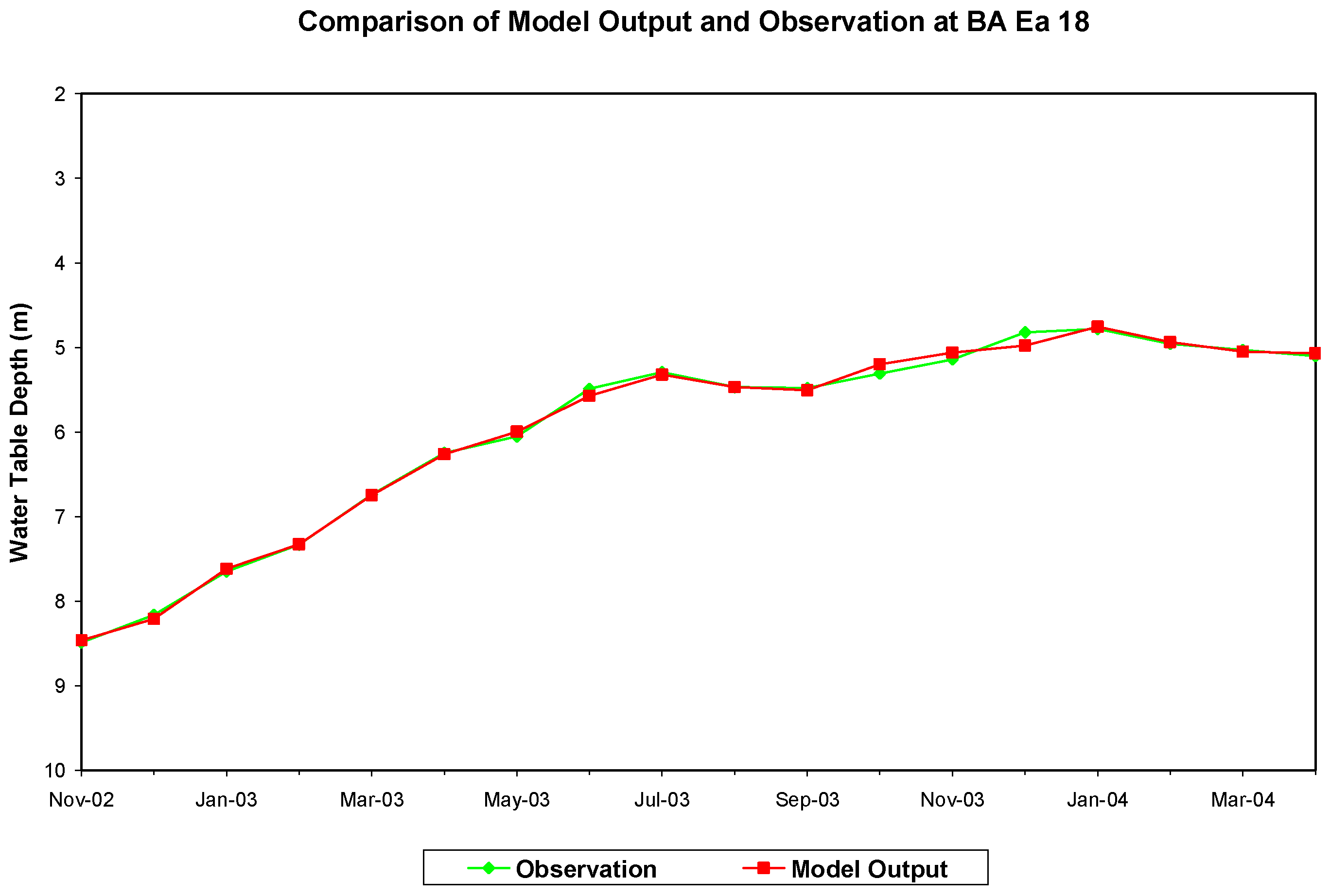
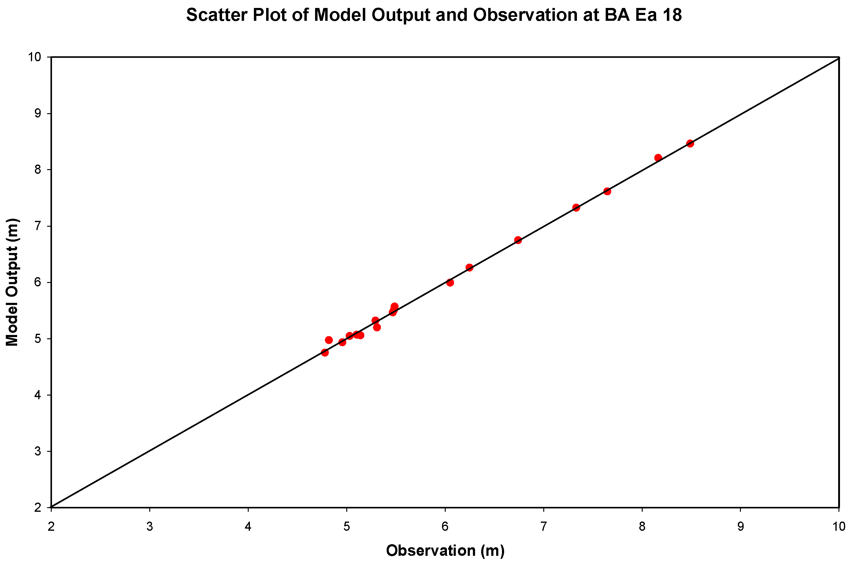
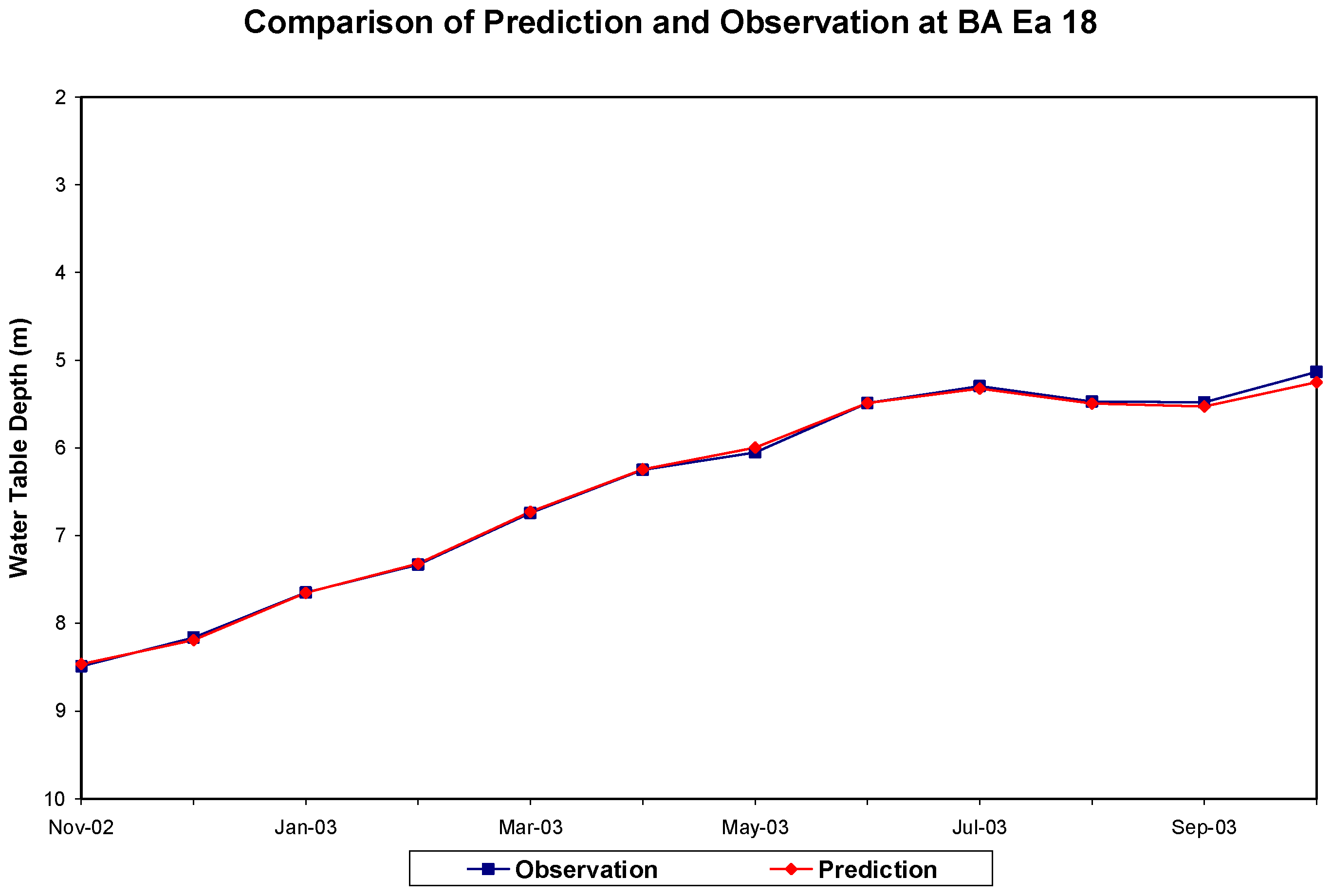
The model was trained with the monthly mean data over the period of November 2002 through April 2004. The training outputs reached a minimum root mean square error of 0.058 m after 350,000 iterations. This ANN model (BA_BT_WT) was selected as the water table prediction model at well site BA Ea 18. The time series of training output of model matches the time series of observation well at this site (Figure 7). A scatter diagram of training output of model against the observed water table depths is also shown in Figure 8. This ANN model was validated by comparing the model’s output with the observed data over the period of May 2004 through October 2004. The validation output resulted in a root mean square error of 0.107 m. The validated water table prediction model’s performance was examined for its forecast capability for the period of November 2002 to October 2003. Except for the predicted water table depth of the subsequent month, the rest of the inputs remained unchanged in the forecast simulations. The comparison between the forecasted and the observed water table depths is shown in Figure 9. A comparison of the forecasted water table depth below ground surface by model BA_BT_WT and the observed data at well site BA Ea 18 shows an RMS error of 0.043 m. Given the graphically illustrated fluctuations in the groundwater table, which are around 3.5 m at this site, an RMSE of 0.043 m signifies a high degree of accuracy in our predictions. This level of precision is particularly notable considering the substantial range of water table fluctuations observed. The absolute difference between the forecasted and the observed water table depths changes from 0.025 m (25 mm) for the first month to 0.116 m (11.6 mm) for the 12th month. The root mean square error of the forecast for 12 months was found to be 0.043 m (43 mm). We believe that these results are very satisfactory considering small difference of 11.6 to 25 mm between the observed and forecasted water tables depths and a low root mean square errors of 43 mm.
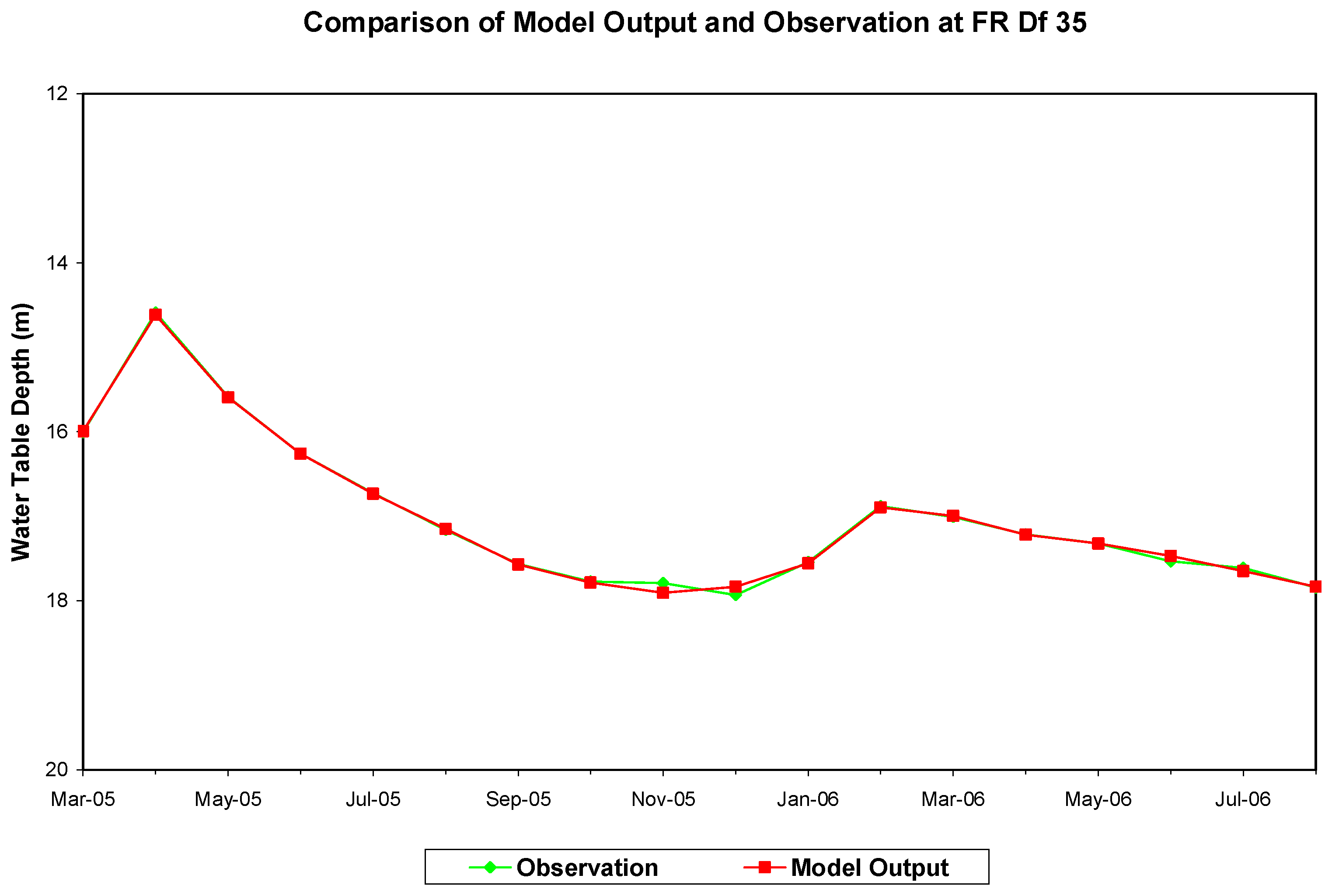
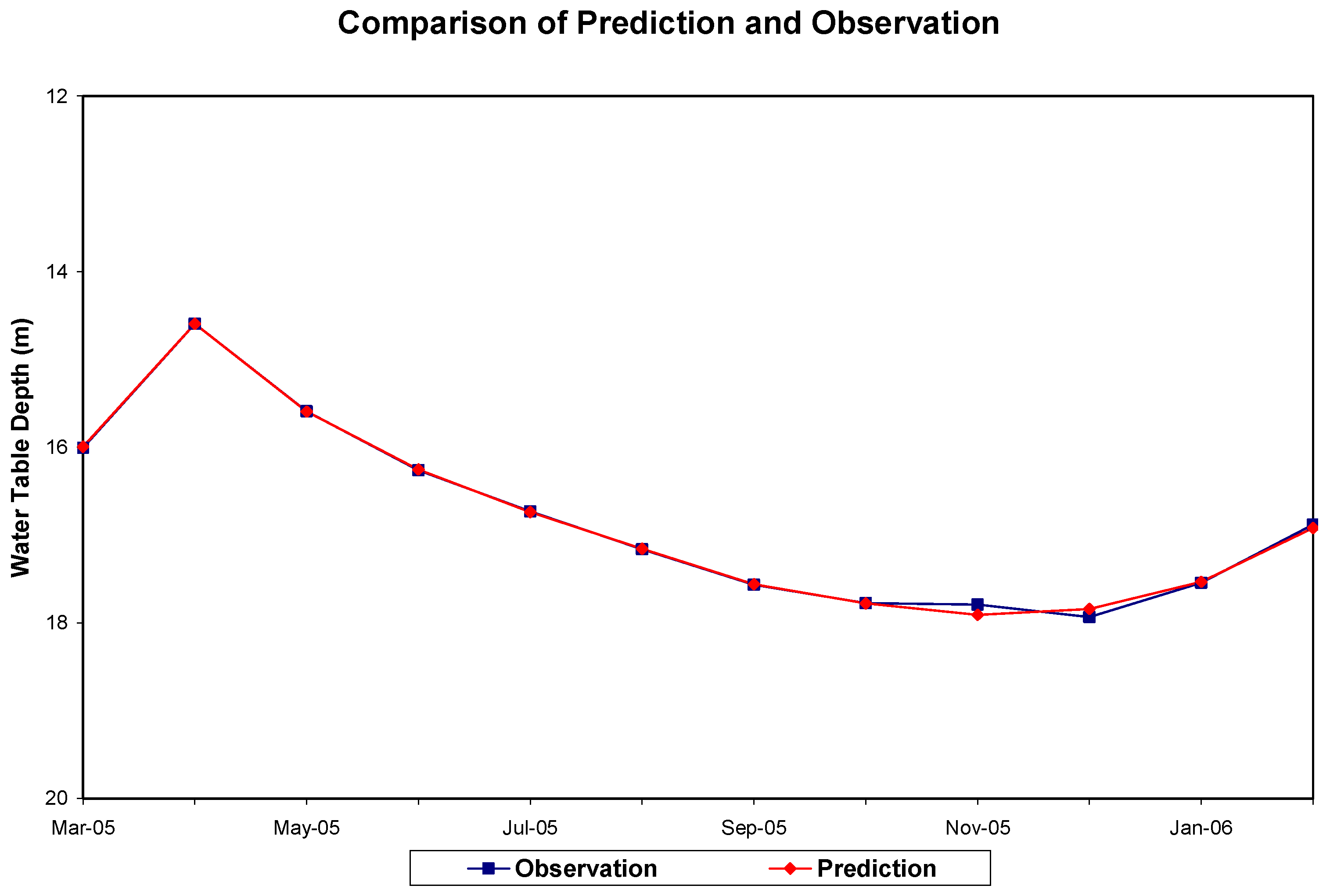
For the purpose of comparison, the same type of model training was conducted in Frederick County, MD at well site FR Df 35. The ANN model structure was the same as that used for BA Ea 18 site. The model was trained with the monthly mean brightness temperature and water table depth over the period from March 2005 to August 2006. The training output came to a minimum root mean square error of 0.04 m (40 mm) after 350,000 iterations. The comparison of the time series of the water table depth resulting from the training phase of the ANN model and the observed water table depth is shown in Figure 10. It demonstrates a good match between these two time series. Figure 11 is the scatter diagram of the model’s output during training against the observed data. Results indicate almost perfect correlation between these two data sets, thus indicating ANN model’s ability in predicting water table depth for the conditions of this study. This ANN model (FR_BT_WT) is thus used as the water table prediction model for this well site. Validation using available data from September 2006 through November 2006 has a root mean square error of 0.089 m (89 mm), indicating a very reasonable performance by the model. Using the validated model, the forecast run was performed over the period from March 2005 to February 2006. The absolute error was found to be 0.009 m (9 mm) and 0.039 m (39 mm) for the first month and 12th month, respectively. The root mean square error over the 12 months’ forecast was determined to be 0.044 m (44 mm), indicating a highly accurate forecasting. This low level of RMSE value (i.e., 44 mm) in light of huge water table fluctuations that are generally over one meter is insignificant, thus showing accuracy of the ANN forecasting model in this study. Figure 12 graphically shows the time series comparison of the forecasted and the observed water table depth for the same well site, FR Df 35 and it clearly indicates very close agreement between the ANN forecasted groundwater tables and the observed values.
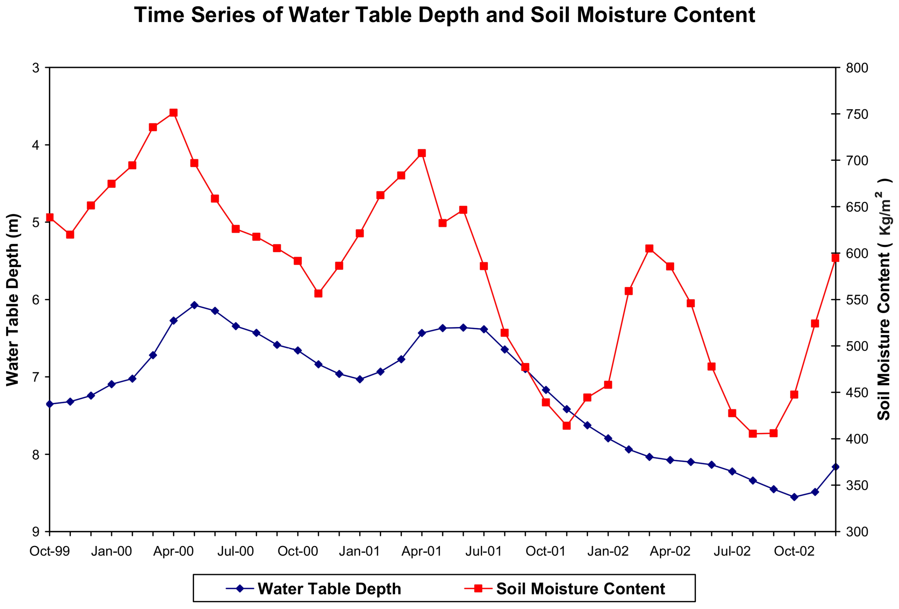
The second attempt in the development of an ANN model for water table prediction utilized monthly mean soil moisture content and monthly mean water table depth as input. Figure 13 shows time series of the monthly mean water table depth and LDAS monthly mean soil moisture content in the topsoil profile (0–2 m) at well site BA Ea 18 in Baltimore County, MD from October 1999 to December 2002. There seems to be a good correlation (r = −0.65) between soil moisture and water table depth. Basically, a water table rise comes with a wet period when soil is moist. The negative r value indicates that higher the soil moisture results in deceased depth from land surface to water table (i.e., high water table) while lower the soil moisture causes increased depth to the water table depth (i.e., low water table).
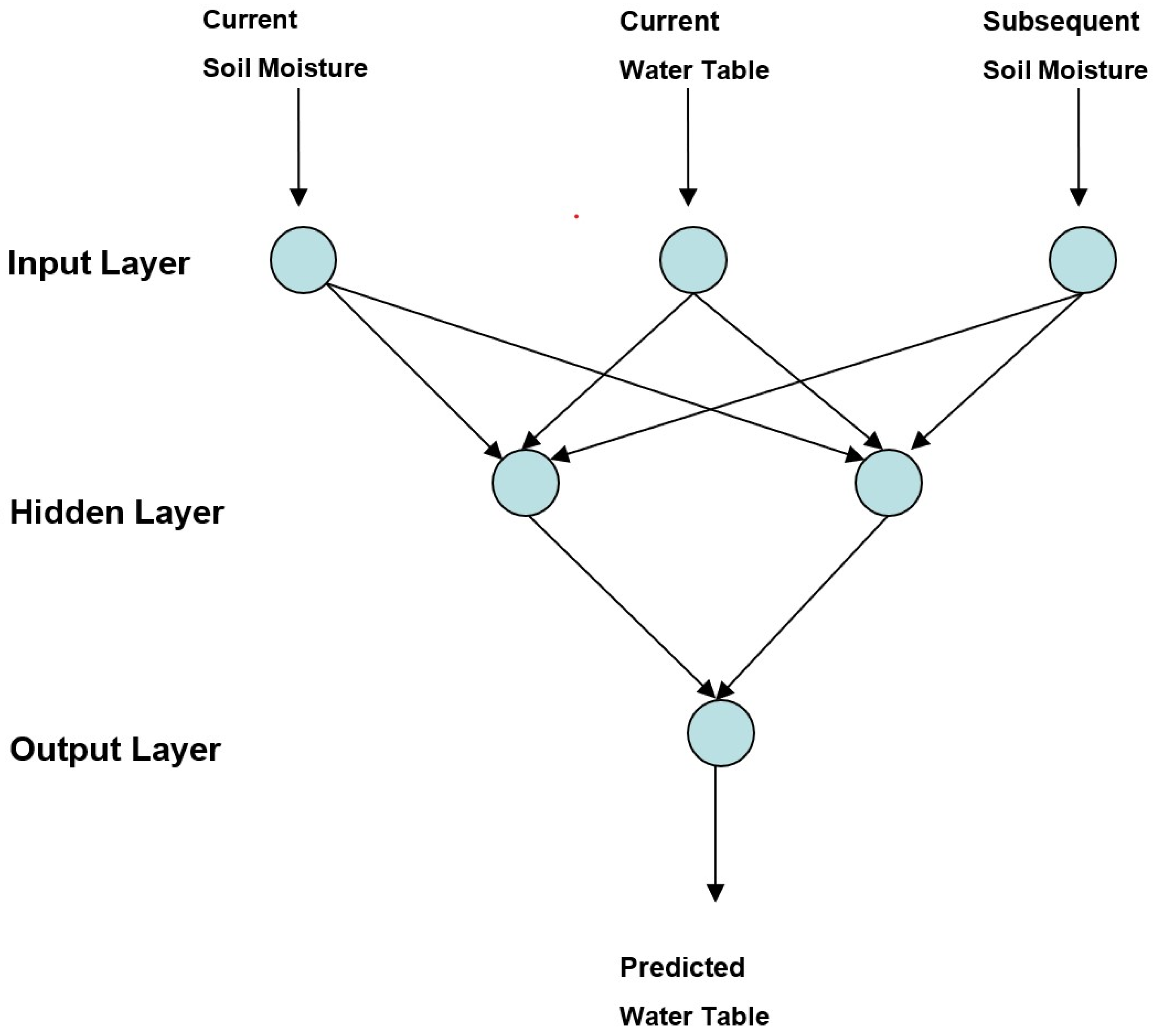
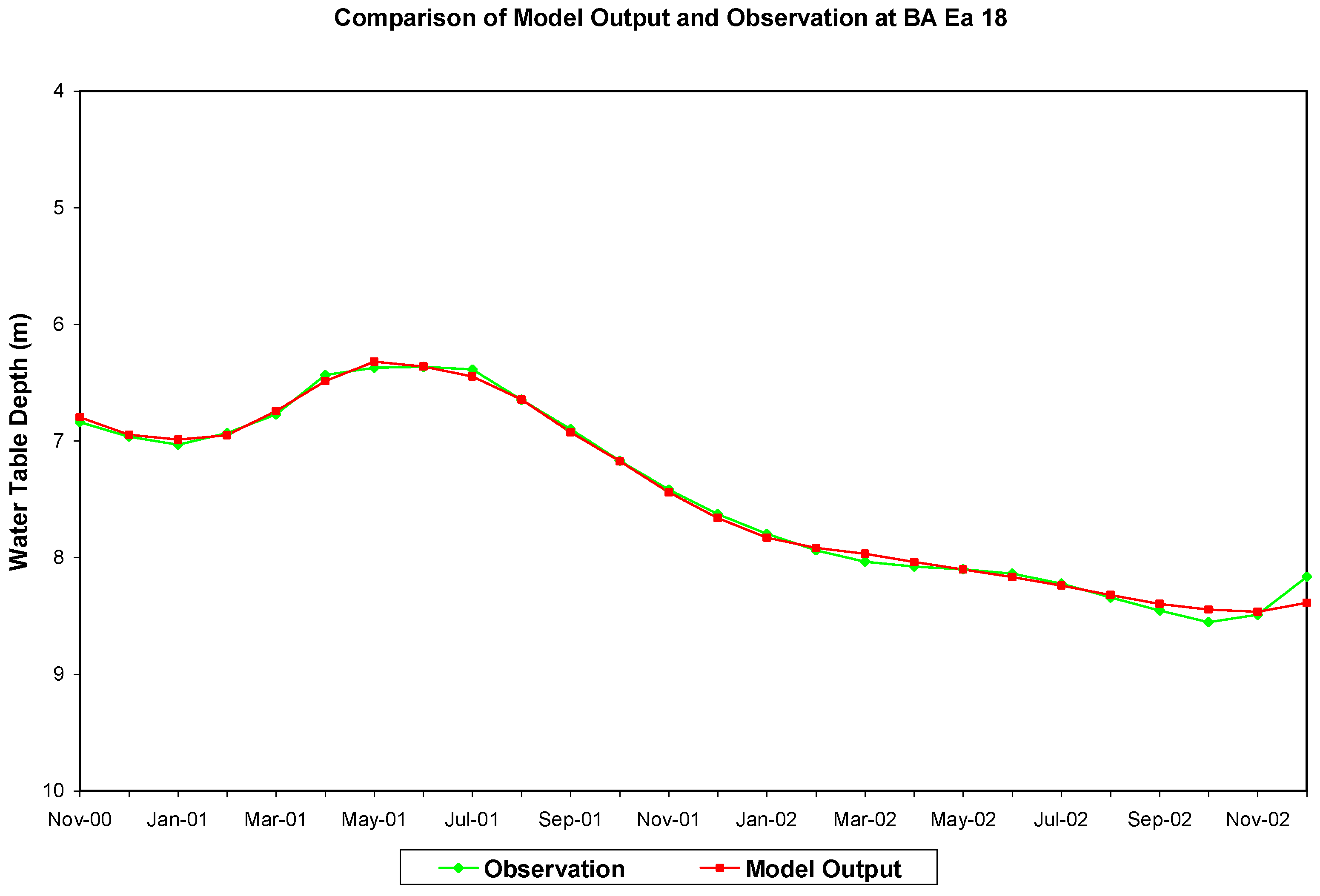
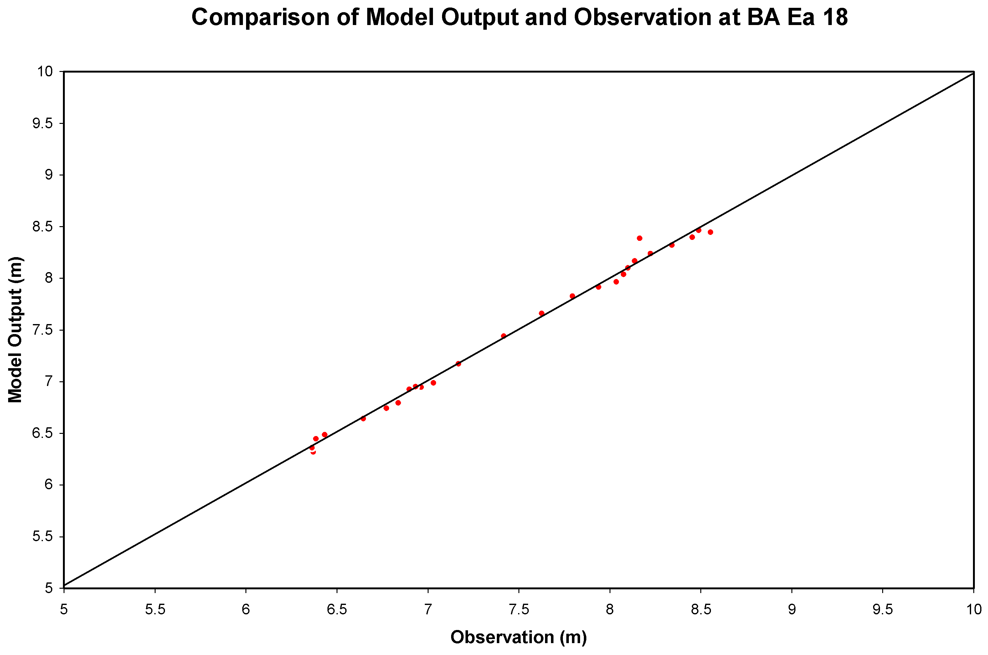
A three-layer feedforward backpropagation ANN with three nodes in the input layer, two nodes in the hidden layer, and one node in the output layer was used to build the ANN model using soil moisture and water table depth as input. The sigmoid function was selected as the activation function. The structure of this ANN model is depicted in Figure 14. Three input nodes are current monthly mean soil moisture, current monthly mean water table depth, and subsequent monthly mean soil moisture. The output node is the predicted water table depth. LDAS monthly mean soil moisture content at the top of the soil profile (0–2 m) and the measured water table depth were used as input to the model. The model was trained with the monthly mean data over the period of November 2000 through December 2002. After 400,000 iterations, the training output reached a minimum root mean square error of 0.059 m (50 mm). Hence, this ANN model (BA_SM_WT) was selected as the water table prediction model. The comparison of the model-predicted water table depth during ANN training with the observation is shown in Figure 15. Results show an excellent match except in the last three months when the water table is low. The scatter plot of the training output against the observation is shown in Figure 16, again indicating a close match. This ANN model was then validated by comparing the model’s output with the observed data over the period from November 1999 through October 2000. The root mean square error of the validation output was 0.069 m (69 mm) which indicates a good prediction. A forecast simulation was conducted for the period from January 2001 to December 2001 to investigate its forecast strength. A comparison of the forecast and the observation is shown in Figure 17. The absolute difference between the forecasted and the observed water table depth ranges from 0.044 m (44 mm) for the first month to 0.089 m (89 mm) for the 12th month. The root mean square error of the forecast over 12 months is 0.047 m (47 mm), all indicating an excellent prediction by the ANN model.

4. Discussion

Two ANN water table prediction models, BA_BT_WT and FR_BT_WT, using brightness temperature and water table depth change as input, were created. Generally, both models predicted water table variation well. The root mean square errors of the model-predicted water table depths during ANN training ranged from 0.04 m (40 mm) for FR_BT_WT to 0.058 m (58 mm) for BA_BT_WT at different well sites. An experiment that used brightness temperature and water table depth for model training was performed, but the results were not acceptable. Results indicated that the relationship between input parameters, as mentioned previously, plays a key factor for the success of this type of modeling. The third ANN model (BA_SM_WT) that utilized soil moisture content and water table depth as input has a root mean square error of 0.059 m (59 mm) for the model training output. Results were compatible with that of the BA_BT_WT’s model. The root mean square errors of the twelve months’ water table depth forecasts are 0.043 m (43 mm), 0.044 m (44 mm), and 0.047 m (47 mm) for BA_BT_WT, FR_BT_WT, and BA_SM_WT, respectively. Comparing with the results of other water table prediction studies [52,53], these results are very encouraging.
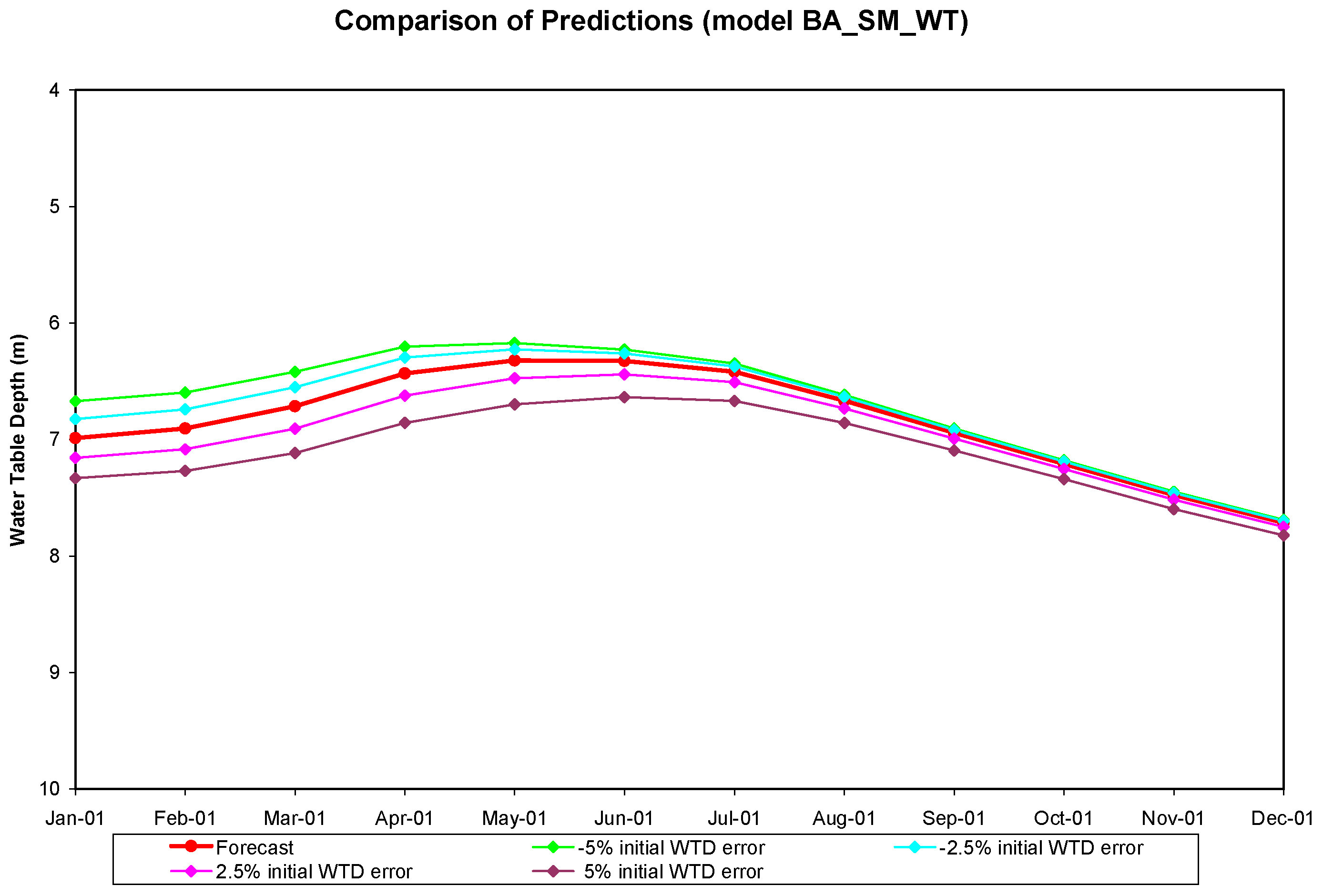
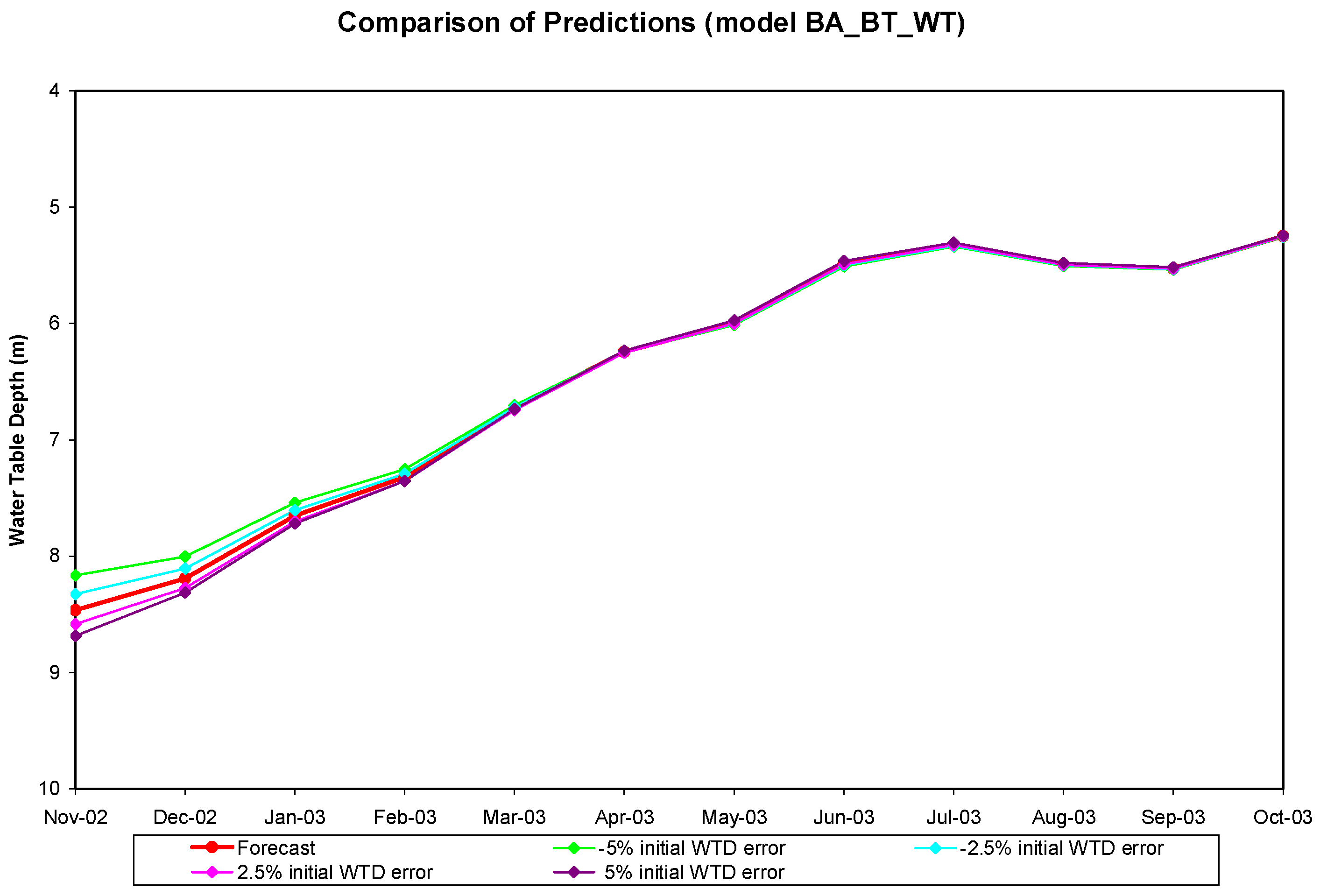
Sensitivity tests were performed for models BA_SM_WT and BA_BT_WT at the Baltimore County well site. BA_SM_WT was tested for the period of January 2001 through December 2001. The monthly mean soil moisture contents remained the same for all cases, but the initial water table depth was assumed to have −5%, −2.5%, 2.5%, or 5% of error for each case of this experiment. After 12 months of model run, the root mean square errors for the monthly predicted output for these four cases were 0.201 m (201 mm), 0.125 m (125 mm), 0.12 m (120 mm), and 0.281 m (281 mm), respectively. They are higher than 0.047 m (47 mm) of the root mean square error of the 12-month long forecast, which started without initial error, for the same time period. The results also showed that the predictions started to converge after 6 months of simulations for all cases (Figure 18). Although they were not fully converged in 12 months, yet it indicates that the influence of the initial error on the input water table depth dissipated after several months of forecasting. A similar test was conducted at the same well site for the period of November 2002 through October 2003 using model BA_BT_WT. The monthly mean brightness temperature remained the same for all cases. The initial water table depth was fed into the model with −5%, −2.5%, 2.5%, or 5% of error for each of these four test cases. The root mean square errors of the 12 months’ predictions for these four cases are 0.121 m (121 mm), 0.068 m (68 mm), 0.061 m (61 mm), and 0.085 m (85 mm), respectively. They are higher than 0.043 m (43 mm) of the 12 months long forecast. The convergence of the predictions occurred at the beginning of the forecast (Figure 19). As the figures show, they completely converged after 5 months of the forecast. This again shows the advantage of applying the ANN model for forecasting long term water table fluctuations. The root mean square errors of models BA_BT_WT and BA_SM_WT are shown in Figure 20. In general, the errors of model BA_BT_WT are larger than that of model BA_SM_WT. This suggests that once higher resolution remotely sensed soil moisture is available, BA_SM_WT might be a better choice for minimizing the effect of possible water table measurement error on the prediction.
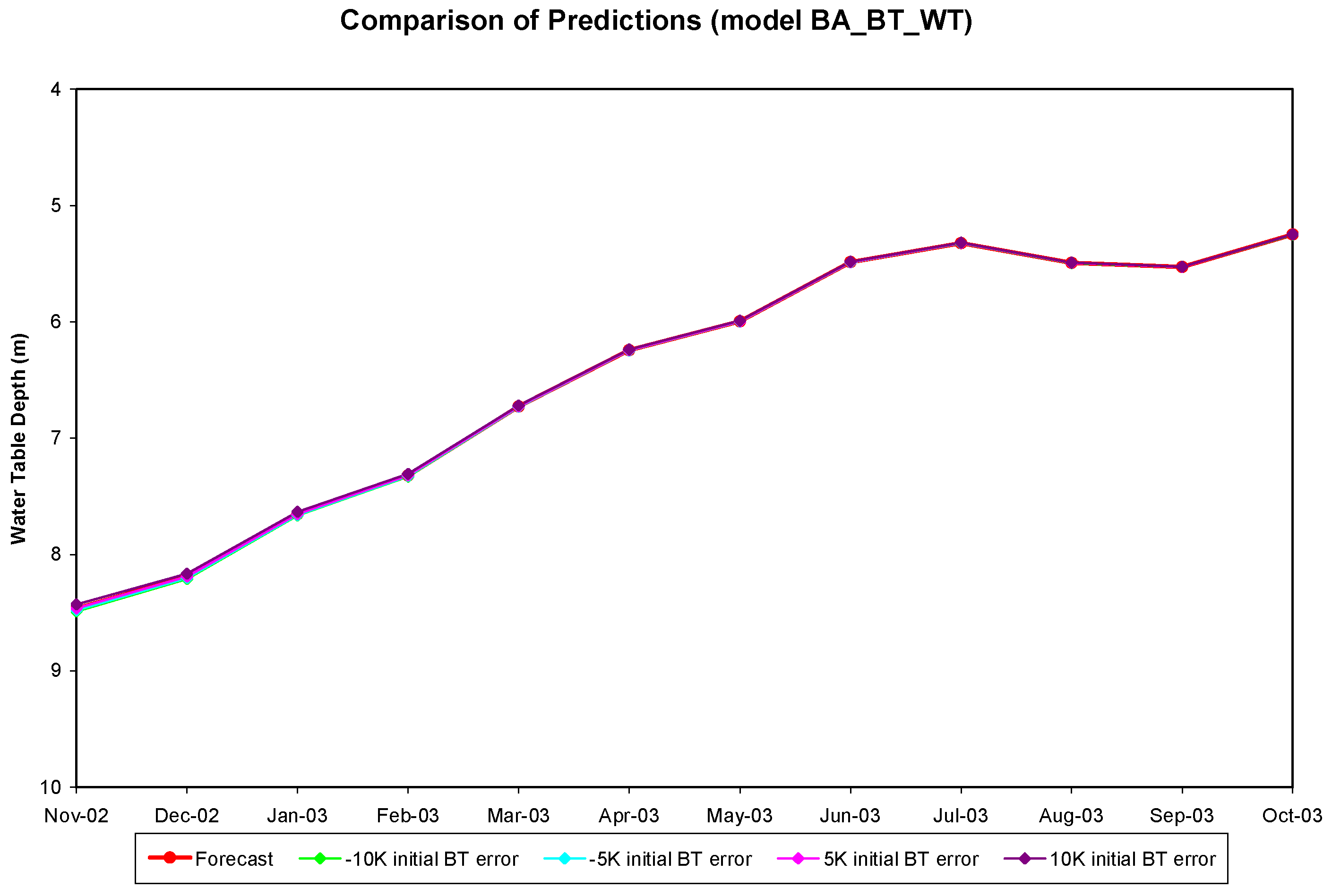
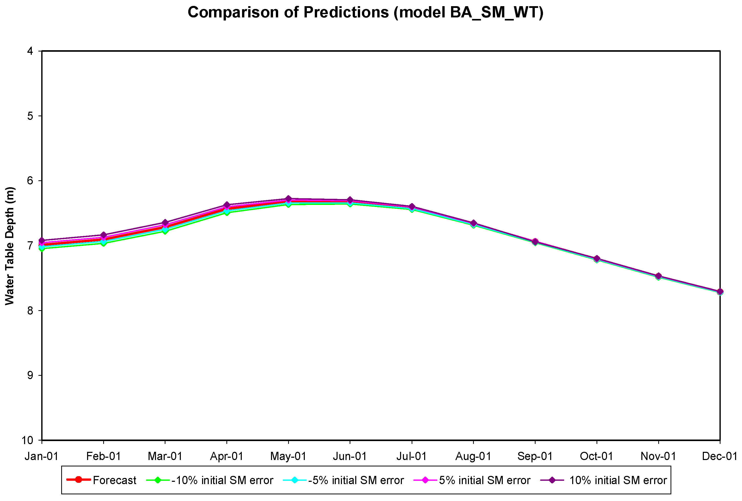
The sensitivity test on brightness temperature was also conducted for the BA_BT_WT model. The test was performed over the period from November 2002 through October 2003. Four cases, each with −10 K, −5 K, 5 K, or 10 K of initial brightness temperature error, were tested. The monthly mean water table depth remained the same for each month. The results showed that there is no significant difference between these four predictions (Figure 21). This indicates that this model is more sensitive to the water table depth error than to the brightness temperature error. Another sensitivity test was performed for the BA_SM_WT model for the period of January 2001 through December 2001 by only changing the initial soil moisture content. For each case, −10%, −5%, 5%, or 10% of error was added onto the initial soil moisture content to determine its impact on the model’s prediction of water table. The comparison of the predicted water table depth of these four tests and the forecast is shown in Figure 22. Data show that the convergence of these predictions occurs at the very beginning and there exists no significant difference among these predictions after 6 months of simulation. The root mean square errors of the monthly predicted water table depth are 0.05 m (50 mm), 0.044 m (44 mm), 0.058 m (58 mm), and 0.076 m (76 mm) for each of these four cases, respectively. Except the second case, they all have higher root mean square errors than that of the forecasted water table depths. All these simulations indicate that the water table depth error, if there is an error, is the major factor affecting ANN model predictions in this study. The influence of the initial brightness temperature error is the least important.
Results obtained in this study are comparable to those obtained by Shamsuddin et al. (2016) where they used multiple input parameters such as daily rainfall, river stage, water level, stream flow rate, temperature, and groundwater level to build their ANN models and predict groundwater fluctuations. Based on the statistical parameters such as coefficient correlation (R), Mean Square Error (MSE), Root Mean Square Error (RMSE) and coefficient determination (R2), they concluded that their models were successful in predicting water table fluctuations. In our study, we were able to build the ANN model with limited number of input parameters such as the brightness temperature and the remotely sensed surface soil moisture and still achieve excellent results as discussed above [54].

5. Conclusions

Three water table depth prediction models which are based on ANN technology were constructed for two locations in Maryland. The sensitivity test results showed that the ANN models developed in this study were more sensitive to the uncertainty in water table depth than both brightness temperature and soil moisture content. This implies that an ANN water table prediction model still can be built once the trend of the time series of the data, such as brightness temperature or soil moisture, over the study site correlates well with that at the study site even if a high resolution remotely sensed data is not available.
The performance of ANN models developed in this study, in general, benefits from better correlation among the input parameters and the target parameter. In addition, the range of the values of the training data, such as water table depth, is crucial on the accuracy of the forecasted water table depths. The prediction might lose its accuracy if the value of the input data is out of the range of the data that trained the model.
The successful application of satellite data on these models for water table fluctuation predictions is very encouraging. A further study that utilizes remotely sensed satellite soil moisture in the model training is needed. An advanced study that extends the ANN water table prediction model to a regional scale is also recommended.
Further investigations could also focus on improving the models’ ability to handle larger fluctuations in water table levels by incorporating more diverse datasets and exploring advanced machine learning techniques. These enhancements will contribute to the development of more accurate and reliable water table prediction tools, crucial for effective water resource management.

Author Contributions

Conceptualization, A.S.; methodology, A.S.; formal analysis, A.S.; writing draft preparation, M.M. and A.S.; writing—review and editing, M.M. and A.S.; visualization, M.M.; supervision, A.S.; project administration, A.S.; funding acquisition, A.S. All authors have read and agreed to the published version of the manuscript.

Funding

This research received no external funding.

Data Availability Statement

Data are available from the authors by request.

Acknowledgments

Authors would like to acknowledge the efforts and time committed by Chung-Yu Wu in building the foundation of this methodology and data used as a part of his Ph.D. research under the supervision of Shirmohammadi in 2007–2008 while a graduate student in the Department of the Biological Resources Engineering at the University of Maryland. Authors tried and searched to locate Wu in order to include him as a co-author in this revised version of the work, but were unable to locate him and find his contact information that is required by the publisher for each co-author. As such, we acknowledge his earlier contributions to the work presented in this manuscript.

Conflicts of Interest

The authors declare no conflicts of interest.

References

  1. Andreasen, D.C.; Nardi, M.R.; Staley, A.W.; Achmad, G.; Grace, J.W. The Maryland Coastal Plain Aquifer Information System: A GIS-based tool for assessing groundwater resources. In Geoscience for the Public Good and Global Development: Toward a Sustainable Future; Wessel, G.R., Greenberg, J.K., Eds.; Geological Society of America: Boulder, CO, USA, 2016; Volume 520, pp. 159–170. [Google Scholar] [CrossRef]
  2. Sanford, W.E.; Pope, J.P.; Selnick, D.L.; Stumvoll, R.F. Simulation of Groundwater Flow in the Shallow Aquifer System of the Delmarva Peninsula, Maryland and Delaware; No. 2012-1140; US Geological Survey: Reston, VA, USA, 2012; p. i-58. [Google Scholar]
  3. Shirmohammadi, A.M.; Rowe, S.; Kasraei, R.; Summers, B.; Michael, R.; Ortt, H.; Schmidt, R.; Shedlock, D.; Nemazi, M.; Negahban–Azar, M.; et al. Stressed Aquifers on the Coastal Plain of Maryland. In Proceedings of the American Geophysical Union (AGU), Quest for Sustainability of Heavily Stressed Aquifers at regional to Global Scales, Valencia, Spain, 21–24 October 2019. [Google Scholar]
  4. Groundwater Protection Program Report to the Maryland General Assembly; Annapolis, MD, USA. 2021. Available online: https://mde.maryland.gov/programs/water/water_supply/Documents/GroundwaterProtectionReport-2021-Dec.pdf (accessed on 9 February 2024).
  5. Chinnasamy, P.; Shiri, J. Groundwater management: Recent advances and applications. J. Hydrol. 2018, 558, 100–111. [Google Scholar]
  6. Kardan Moghaddam, H.; Kardan Moghaddam, H.; Rahimzadeh Kivi, Z.; Bahreinimotlagh, M.; Alizadeh, M.J. Developing comparative mathematic models, BN and ANN for forecasting of groundwater levels. Groundw. Sustain. Dev. 2019, 9, 100237. [Google Scholar] [CrossRef]
  7. Zhang, M.; Wang, Y.; Wang, X.; Zhou, W. Groundwater depth forecasting using a coupled model. Discret. Dyn. Nat. Soc. 2021, 2021, 6614195. [Google Scholar] [CrossRef]
  8. Li, W.; Bao, L.; Yao, G.; Wang, F.; Guo, Q.; Zhu, J.; Zhu, J.; Wang, Z.; Bi, J.; Zhu, C.; et al. The analysis on groundwater storage variations from GRACE/GRACE-FO in recent 20 years driven by influencing factors and prediction in Shandong Province, China. Sci. Rep. 2024, 14, 5819. [Google Scholar] [CrossRef]
  9. Mirzavand, M.; Ghazavi, R.A. Stochastic Modelling Technique for Groundwater Level Forecasting in an Arid Environment Using Time Series Methods. Water Resour. Manag. 2015, 29, 1315–1328. [Google Scholar] [CrossRef]
  10. Mogaji, K.A.; Lim, H.S.; Abdullah, K. Modeling of groundwater recharge using a multiple linear regression (MLR) recharge model developed from geophysical parameters, a case of groundwater resources management. Environ. Earth Sci. 2015, 73, 1217–1230. [Google Scholar] [CrossRef]
  11. Patle, G.T.; Singh, D.K.; Sarangi, A.; Rai, A.; Khanna, M.; Sahoo, R.N. Time series analysis of groundwater levels and projection of future trend. J. Geol. Soc. India 2015, 85, 232–242. [Google Scholar] [CrossRef]
  12. Patel, P.; Kumar, P.; Rajni. The numerical solution of Boussinesq equation for shallow water waves. AIP Conf. Proc. 2020, 2214, 020019. [Google Scholar] [CrossRef]
  13. Pozdniakov, S.P.; Wang, P.; Grinevsky, S.O.; Frolova, N.L. A Physically Based Model of a Two-Pass Digital Filter for Separating Groundwater Runoff From Streamflow Time Series. Water Resour. Res. 2022, 58, e2021WR031333. [Google Scholar] [CrossRef]
  14. Ebel, B.A.; Shephard, Z.M.; Walvoord, M.A.; Murphy, S.F.; Partridge, T.F.; Perkins, K.S. Modeling Post-Wildfire Hydrologic Response: Review and Future Directions for Applications of Physically Based Distributed Simulation. Earth’s Future 2023, 11, e2022EF003038. [Google Scholar] [CrossRef]
  15. Vujevic, K.; Deissinger, P.; Klocking, B.; Pfutzner, B.; Weiss, J. Regional water balance modelling to evaluate future groundwater management. Grundwasser 2023, 28, 271–285. [Google Scholar] [CrossRef]
  16. Scheibe, C. Groundwater- and surface water balance in aquifers of the ostliche Bodenwohrer Senke, Oberpfalz. Water Resour. Manag. 2022, 27, 171–185. [Google Scholar] [CrossRef]
  17. Abebe, W.T. Evaluation of groundwater resource potential by using water balance model: A case of Upper Gilgel Gibe Watershed, Ethiopia. Water Resour. Power 2022, 10, 209–222. [Google Scholar] [CrossRef]
  18. Ye, Y.; Chen, W.; Wang, G.R.; Xue, W.F. Spatial Prediction of the Groundwater Potential Using Remote Sensing Data and Bivariate Statistical-Based Artificial Intelligence Models. Water Resour. Manag. 2022, 36, 5461–5494. [Google Scholar] [CrossRef]
  19. Eslami, P.; Nasirian, A.; Akbarpour, A.; Tahroudi, M.N. Groundwater estimation of Ghayen plain with regression-based and hybrid time series models. Paddy Water Environ. 2022, 20, 429–440. [Google Scholar] [CrossRef]
  20. Tsuchihara, T.; Yoshimoto, S.; Shirahata, K.; Nakazato, H.; Ishida, S. Analysis of groundwater-level fluctuation and linear regression modeling for prediction of initial groundwater level during irrigation of rice paddies in the Nasunogahara alluvial fan, central Japan. Environ. Earth Sci. 2023, 82, 473. [Google Scholar] [CrossRef]
  21. Shirmohammadi, A.; Chaubey, I.; Harmel, R.D.; Bosch, D.D.; Munoz-Carpena, R.; Dharmarsi, C.; Sexton, A.; Arabi, M.; Wolfe, M.L.; Frankenberger, J.; et al. Uncertainity in TMDL Models. Trans. ASABE 2006, 494, 1033–1049. [Google Scholar] [CrossRef]
  22. Medawela, S.; Armaghani, D.J.; Indraratna, B.; Rowe, R.K.; Thamwattana, N. Development of an ad-vanced machine learning model to predict the pH of groundwater in permeable reactive barriers (PRBs) located in acidic terrain. Comput. Geotech. 2023, 161, 105557. [Google Scholar] [CrossRef]
  23. Sahoo, S.; Jha, M.K. Groundwater-level prediction using multiple linear regression and artificial neural network techniques: A comparative assessment. Hydrogeol. J. 2013, 21, 1865–1887. [Google Scholar] [CrossRef]
  24. Suryanarayana, C.; Sudheer, C.; Mahammood, V.; Panigrahi, B.K. An integrated wavelet-support vector ma-chine for groundwater level prediction in Visakhapatnam, India. Neurocomputing 2014, 145, 324–335. [Google Scholar] [CrossRef]
  25. Wen, X.; Feng, Q.; Yu, H.; Wu, J.; Si, J.; Chang, Z.; Xi, C. Wavelet and adaptive neuro-fuzzy inference system conjunction model for groundwater level predicting in a coastal aquifer. Neural Comput. Appl. 2015, 26, 1203–1215. [Google Scholar] [CrossRef]
  26. Zhang, J.; Zhu, Y.; Zhang, X.; Ye, M.; Yang, J. Developing a Long Short-Term Memory (LSTM) based model for predicting water table depth in agricultural areas. J. Hydrol. 2018, 561, 918–929. [Google Scholar] [CrossRef]
  27. Emamgholizadeh, S.; Moslemi, K.; Karami, G. Prediction the Groundwater Level of Bastam Plain (Iran) by Artificial Neural Network (ANN) and Adaptive Neuro-Fuzzy Inference System (ANFIS). Water Resour. Manag. 2014, 15, 5433–5446. [Google Scholar] [CrossRef]
  28. Dogan, A.; Demirpence, H.; Cobaner, M. Prediction of groundwater levels from lake levels and climate data using ANN approach. Water SA 2008, 34, 199–208. [Google Scholar] [CrossRef]
  29. Reuter, U.; Moller, B. Artificial Neural Networks for Forecasting of Fuzzy Time Series. Comput.-Aided Civ. Infrastruct. Eng. 2010, 25, 363–374. [Google Scholar] [CrossRef]
  30. Shirmohammadi, B.; Vafakhah, M.; Moosavi, V.; Moghaddamnia, A. Application of several data-driven techniques for predicting groundwater level. Water Resour. Manag. 2012, 27, 419–432. [Google Scholar] [CrossRef]
  31. Kuo, J.T.; Hsieh, M.H.; Lung, W.S.; She, N. Using artificial neural network for reservoir eutrophication prediction. Ecol. Model. 2006, 200, 171–177. [Google Scholar] [CrossRef]
  32. Alzahrani, R.A.; Parker, A.C. Neuromorphic Circuits With Neural Modulation Enhancing the Information Content of Neural Signaling. In Proceedings of the International Conference on Neuromorphic Systems 2020 (ICONS 2020), Association for Computing Machinery, New York, NY, USA, 28–30 July 2020; pp. 1–8. [Google Scholar] [CrossRef]
  33. Salami, E.S.; Ehteshami, M. Simulation, evaluation and prediction modeling of river water quality properties (case study: Ireland Rivers). Int. J. Eng. Sci. Technol. 2015, 12, 3235–3242. [Google Scholar] [CrossRef]
  34. Ehteshami, M.; Dolatabadi, N.F.; Tavassoli, S. Simulation of nitrate contamination in groundwater using artificial neural networks. Model Earth Syst. Environ. 2016, 2, 28. [Google Scholar] [CrossRef]
  35. Sarkar, A.; Pandey, P. River water quality modelling using artificial neural network technique. International conference on water resources, coastal and ocean engineering (icwrcoe 2015). Aquat. Procedia 2015, 4, 1070–1077. [Google Scholar] [CrossRef]
  36. Daliakopoulos, I.N.; Coulibaly, P.; Tsanis, I.K. Groundwater level forecasting using artificial neural networks. J. Hydrol. 2005, 309, 229–240. [Google Scholar] [CrossRef]
  37. Mohanty, S.; Jha, M.K.; Kumar, A.; Panda, D.K. Comparative evaluation of numerical model and artificial neural network for simulating groundwater flow in Kathajodi-Surua Inter-basin of Odisha India. J. Hydrol. 2013, 495, 38–51. [Google Scholar] [CrossRef]
  38. Shiri, J.; Kisi, O.; Yoon, H.; Lee, K.K.; Nazemi, A.H. Predicting groundwater level fluctuations with meteorological effect implications—A comparative study among soft computing techniques. Comput. Geosci. 2013, 56, 32–44. [Google Scholar] [CrossRef]
  39. NSIDC. Home Page. 2008. Available online: http://nsidc.org/daac/projects/passivemicro/amsre.html (accessed on 15 February 2008).
  40. USGS. Water Resources Data: Maryland and Delaware Water Year 2001; Ground-Water Data, USGS Water-Data Report MD-DE-01-2; USGS: Reston, VA, USA, 2021; Volume 2. [Google Scholar]
  41. Ashcroft, P.; Wentz, F. Updated Daily. AMSR-E/Aqua L2A Global Swath Spatially-Resampled Brightness Temperatures V002, Mar 2008; Digital Media; National Snow and Ice Data Center: Boulder, CO, USA, 2006. [Google Scholar]
  42. Mitchell, K.; Houser, P.; Wood, E.; Schaake, J.; Tarpley, D.; Lettenmaier, D.; Higgins, W.; Marshall, C.; Lohmann, D.; Ek, M.; et al. GCIP Land Data Assimilation Systems (LDAS) Project Now Underway; World Climate Research Programme; GEWEX News: Fairfax, VA, USA, 1999. [Google Scholar]
  43. Selker, J.S.; Keller, C.K.; McCord, J.T. Vadose Zone Processes; Lewis Publishers: Boca Raton, FL, USA, 1999; p. 339. [Google Scholar]
  44. Schmugge, T.; Gloersen, P.; Wilheit, T.; Geiger, F. Remote Sensing of Soil Moisture with Microwave Radiometers. J. Geophys. Res. 1974, 79, 317–323. [Google Scholar] [CrossRef]
  45. Schmugge, T. Remote Sensing of Surface Soil Moisture. J. Appl. Meteorol. 1978, 17, 1549–1557. [Google Scholar] [CrossRef]
  46. Wang, H.; Li, Z.; Zhang, W.; Ye, X.; Liu, X. A Modified Temperature-Vegetation Dryness Index (MTVDI) for Assessment of Surface Soil Moisture Based on MODIS Data. Chin. Geogr. Sci. 2022, 32, 592–605. [Google Scholar] [CrossRef]
  47. Gao, Y.; Lian, X.; Ge, L. Inversion model of surface bare soil temperature and water content based on UAV thermal infrared remote sensing. Infrared Phys. Technol. 2022, 125, 104289. [Google Scholar] [CrossRef]
  48. Ahmadi, S.; Alizadeh, H.; Mojaradi, B. Land surface temperature assimilation into a soil moisture-temperature model for retrieving farm-scale root zone soil moisture. Geoderma 2022, 421, 115923. [Google Scholar] [CrossRef]
  49. Zou, J.; Gao, J.; Wei, J.; Fan, C. Soil moisture monitoring based on long-term time series land surface temperature (LST) data-a case study in Hebi city, Henan province. Bangladesh J. Bot. 2020, 49, 735–742. [Google Scholar]
  50. Svozil, D.; Kvasnicka, V.; Pospichal, J. Introduction to multi-layer feed-forward neural networks. Chemom. Intell. Lab. Syst. 1997, 39, 43–62. [Google Scholar] [CrossRef]
  51. Socha, P.; Miškovský, V.; Kubátová, H.; Novotný, M. Correlation Power Analysis Distinguisher Based on the Correlation Trace Derivative. In Proceedings of the 2018 21st Euromicro Conference on Digital System Design (DSD), Prague, Czech Republic, 29–31 August 2018; pp. 565–568. [Google Scholar] [CrossRef]
  52. Fausett, L. Fundamentals of Neural Networks: Architectures, Algorithms, and Applications; Prentice-Hall: Englewood Cliffs, NJ, USA, 1994. [Google Scholar]
  53. Coulibaly, P.; Anctil, F.; Aravena, R.; Bobee, B. Artificial neural network modeling of water table depth fluctuations. Water Resour. Res. 2001, 37, 885–896. [Google Scholar] [CrossRef]
  54. Shamsuddin MK, N.; Kusin, F.M.; Sulaiman, W.N.A.; Ramli, M.F.; Baharuddin MF, T.; Adnan, M.S. Forecasting of Groundwater Level using Artificial Neural Network by incorporating river recharge and river bank infiltration. In MATEC Web of Conferences; EDP Sciences: London, UK, 2017; Volume 103, p. 04007. [Google Scholar]
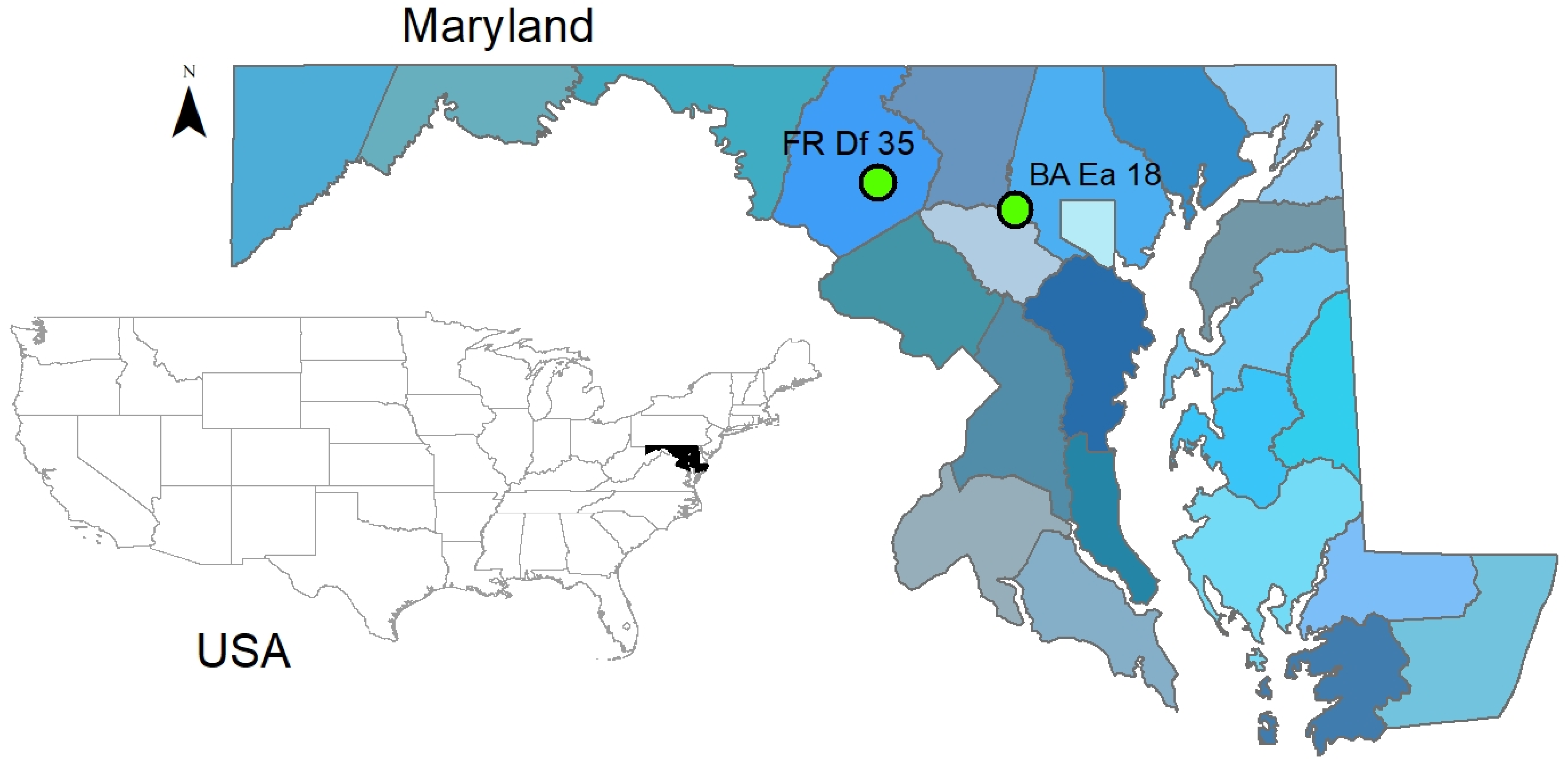
Figure 1. The geographical location of groundwater wells utilized in this study.
Water 16 01500 g001
Figure 2. A schematic diagram of a three-layer ANN model using previous brightness temperature (BT1), current brightness temperature (BT2), water table depth change (WT2–WT1), current water table depth (WT2), and subsequent brightness temperature (BT3) as input. The output is predicted water table depth (WT3).
Water 16 01500 g002
Figure 3. The time series of water table depth (below the ground surface) and brightness temperature at well site BA Ea 18 in Baltimore County, MD (r = −0.17).
Water 16 01500 g003
Figure 4. The Time series of water table depth change and brightness temperature at well site BA Ea 18 in Baltimore County, MD (r = 0.53).
Water 16 01500 g004
Figure 5. The time series of water table depth below ground surface and brightness temperature at well site FR Df 35 in Frederick County, MD (r = 0.05).
Water 16 01500 g005
Figure 6. The time series of water table depth change and brightness temperature at well site FR Df 35 in Frederick County, MD (r = 0.56).
Water 16 01500 g006
Figure 7. Comparison of the model-predicted water table depth (below ground surface) during ANN training with the observation at well site BA Ea 18.
Water 16 01500 g007
Figure 8. The scatter diagram of the model-predicted water table depth during ANN training against the observed water table depth at well site BA Ea 18.
Water 16 01500 g008
Figure 9. A comparison of the forecasted water table depth below ground surface (by model BA_BT_WT) and the observed data at well site BA Ea 18. The forecast has an RMS error of 0.043 m.
Water 16 01500 g009
Figure 10. Comparison of the model-predicted water table depth during ANN training with the observation at well site FR Df 35.
Water 16 01500 g010
Figure 11. The scatter diagram of the model-predicted water table depth during ANN training against the observed water table depth at well site FR Df 35.
Water 16 01500 g011
Figure 12. A comparison of the forecasted water table depth below ground surface (by model FR_BT_WT) and the observed data at well site FR Df 35. The forecast has a RMS error of 0.044 m.
Water 16 01500 g012
Figure 13. The time series of water table depth below ground surface and soil moisture content at well BA Ea 18 in Baltimore County, MD (r = −0.65).
Water 16 01500 g013
Figure 14. A schematic diagram of a three-layer ANN model using current soil moisture content, current water table depth, and subsequent soil moisture content as input. The output is predicted water table depth.
Water 16 01500 g014
Figure 15. Comparison of the model-predicted water table depth (below ground surface) during ANN training with the observation at well site BA Ea 18.
Water 16 01500 g015
Figure 16. The scatter diagram of the model-predicted water table depth below ground surface during ANN training against the observed water table depth at well site BA Ea 18.
Water 16 01500 g016
Figure 17. A comparison of the forecasted water table depth below ground surface (by model BA_SM_WT) and the observed data at well site BA Ea 18. The forecast has an RMS error of 0.047 m.
Water 16 01500 g017
Figure 18. The comparison of predicted monthly water table depths below g round surface generated by running ANN model BA_SM_WT with different errors on initial water table depths (WTD).
Water 16 01500 g018
Figure 19. The comparison of predicted monthly water table depths below ground surface generated by running ANN model BA_BT_WT with different errors on initial water table depths (WTD).
Water 16 01500 g019
Figure 20. Root mean square errors of 12 months’ predicted water table depths below ground surface generated by models BA_BT_WT and BA_SM_WT at different initial water table depth errors.
Water 16 01500 g020
Figure 21. The comparison of predicted monthly water table depths below ground surface generated by running ANN model BA_BT_WT with different errors on initial brightness temperature (BT).
Water 16 01500 g021
Figure 22. The comparison of predicted monthly water table depths below ground surface generated by running ANN model BA_SM_WT with different errors on initial soil moisture content (SM).
Water 16 01500 g022
Disclaimer/Publisher’s Note: The statements, opinions and data contained in all publications are solely those of the individual author(s) and contributor(s) and not of MDPI and/or the editor(s). MDPI and/or the editor(s) disclaim responsibility for any injury to people or property resulting from any ideas, methods, instructions or products referred to in the content.