Article

Developing Regional Hydrological Drought Risk Models through Ordinary and Principal Component Regression Using Low-Flow Indexes in Susurluk Basin, Turkey

by
Çiğdem Gürler
1,2,
Alper Serdar Anli
3,4,* and
Havva Eylem Polat
3
1
General Directorate of Water Management, Ministry of Agriculture and Forestry, 06510 Ankara, Turkey
2
Agricultural Structures and Irrigation Department, Graduate School of Natural and Applied Sciences, Ankara University, 06560 Ankara, Turkey
3
Agricultural Structures and Irrigation Department, Agricultural Faculty, Ankara University, 06560 Ankara, Turkey
4
Water Management Institute, Ankara University, 06560 Ankara, Turkey
*
Author to whom correspondence should be addressed.
Water 2024, 16(11), 1473; https://doi.org/10.3390/w16111473
Submission received: 1 May 2024 / Revised: 18 May 2024 / Accepted: 20 May 2024 / Published: 22 May 2024
(This article belongs to the Special Issue Statistical Modelling of Hydrological Extremes: Floods and Droughts)

Abstract

:
Susurluk Basin is among the basins that may be most affected by drought risk due to its agricultural, economic, and natural resources. In this study, regional hydrological drought risk models were developed for water supply systems in the Susurluk Basin, Turkey. Twenty-four flow observation sites with 25 years or more of data showing natural flow characteristics as much as possible were converted into daily flow data with Q7, Q15, Q30, and Q60 low-flow indexes. Regionalization was carried out by two-stage multivariate cluster and principal component analysis using the basins’ physical and hydrological characteristics and low-flow statistics, and two homogeneous regions were obtained due to the discordancy, heterogeneity, and goodness of fit tests, which are L-moment approaches. Regional models were performed with ordinary and principal component regression techniques using the physical and hydrological characteristics of the watersheds and regional low-flow frequency analysis. The cross-validation procedure results for ungauged basins show that ordinary regression models are more effective in the lowland first region. In contrast, principal component regression models are more suitable for the mountainous second region. This study’s findings, which are a first for the Susurluk Basin, will have important results in terms of agricultural water management in the region and will help the water authority in water allocation. To investigate whether human impact and climate change impact the prediction of hydrological drought, we recommend seasonal non-stationary frequency analysis with the addition of useful empirical hydrological drought indexes.

1. Introduction

Low flow is the state of decreasing flow in a stream, and it is an extreme hydrological process that is usually observed in the summer and changes randomly every year. On the other hand, drought is a natural event that adversely affects land and resource production systems and causes serious hydrological imbalances due to precipitation falling significantly below the recorded normal levels [1]. While low flows may be observed during dry periods, not all low flows indicate drought. However, drought can be observed due to the overlapping of low flows over a period of time. Low-flow studies are important in taking measures that can reduce the negative effects of dry periods. Low-flow analysis studies can be used in water resources and water quality management, determining management strategies, regional analysis of surface water resources, designing water supply facilities within confidence limits, and calculating the minimum tail water that should be left downstream in hydraulic structures [2,3].
Low-flow analyses can be made using two different analysis methods: hydrological and statistical. In hydrological analysis, flow duration curves are drawn with the mean lowest flow values obtained using d-day flow rates, and values corresponding to 90%, 95%, and 99% of the observation period are determined [4]. Statistical low-flow analysis is performed by frequency analysis of d-day flow values and determining appropriate probability distributions. These hydrological and statistical approaches can also combine low-flow statistics with the physiographic–hydrological characteristics of watersheds to transfer them to ungauged sites [5]. The frequency of occurrence of hydrological events is determined by frequency analysis, and it is preferred that the flow data used in these studies be as continuous and uninterrupted as possible. Low flow in a stream is generally defined by the magnitude of flow and the frequency and duration of reductions in flow. Determining the magnitude and duration of low flow with a given probability of occurrence is important in hydrological modeling and water resource management. However, this may not be the case in many cases because the data set is short or more sites are needed. Regionalization techniques have been developed to augment limited data or to estimate flow data at ungauged locations [6].
The concept of using minimum d-day low flows in the low-flow analysis was first proposed by [7]. Generally, 7-day low flows are preferred for drought and water resource management because they give better results. There are also studies related to low-flow analysis, such as [8,9,10,11,12,13]. Ref. [14] is one of the main studies within the scope of low-flow studies and touches on low-flow analysis and the regionalization of these analyses. The study explains methods such as base flow index, flow duration curves, and flow-frequency curves through flow measurements, and many of today’s methods have been developed based on these studies. Ref. [15] conducted low-flow studies at 184 sites in southeastern Australia. In this study, he tried to determine the link between low-flow parameters, climate, and location data. On the other hand, by improving his previous studies, the author in [16] tried to develop a methodology between low-flow characteristics in small-scale rural basins that could not be measured and their reflections in the basin. In this study, a regionalization was conducted to determine hydrologically similar properties and develop appropriate equations. Another fundamental study related to low-flow analysis methods is [17]. He evaluated the low-flow studies conducted in the 1980s and later and the techniques used in these studies. He touched upon issues such as low-flow formation, estimation and interpretation of low flows, and detection of low flows in basins without flow measurement. Ref. [18] used the Wakeby probability distribution function to detect low-flow periods and perform low-flow frequency analysis in ungauged basins in Colombia. This distribution was chosen because it is flexible compared to other distribution functions and gives positive returns at extreme values. Ref. [19] emphasized that low-flow estimation studies are of great importance in assessing the availability of water resources. In their study, they investigated the applicability of physiographic space-based interpolation techniques for the estimation of low-flow indexes in ungauged basins. As the study area, they preferred a wide region to cover 51 basins in central Italy. As a result of the study, they found that physiographic space-based interpolation is a suitable approach for estimating low-flow indexes in ungauged basins, and geostatistics techniques outperform deterministic techniques. Ref. [20] studied the classification of low-flow regimes at a regional scale in semi-arid areas in Europe. They conducted analyses using flow duration curves and monthly flow series in this context. Ref. [21] carried out a series of studies, including quality analysis at metered sites, low-flow frequency analysis, and creating a global model to evaluate the physical parameters of the basin and low-flow indexes. They obtained four different homogeneous regions in the study area. They emphasized that the study result could have been healthier due to the limited number of sites with 20 years or more of data within the study’s scope. It would be beneficial to update the study when data availability is ensured. Ref. [22] studied principal component analysis with 13 dimensionless geomorphological parameters in 8 sub-basins of the Kanhiya Nala basin of India and grouped the parameters under different components depending on their correlations. Principal component analysis results revealed that 11 of these parameters were strongly related to the components. Ref. [23] carried out a study in which possible changes in drought and low-flow rates in the future were determined, considering the effects of climate change. The Netherlands, Switzerland, Italy, Portugal, Spain, and some regions of Greece were defined as the study areas. The study concludes that low flow will likely become excessive and more intense hydrological droughts will develop.
Looking at the low-flow studies in Turkey, Ref. [4] discussed the basic conceptual issues related to low flows. A low-flow statistical analysis was carried out by [24,25] in the Thrace Region and [26] in the Sakarya [27] and Meriç Basins [28]. In addition, a low-flow statistical analysis was carried out by [29] in the Aegean Region, by [30] in the Mediterranean Region, by [31] in the Yeşilırmak Basin, and by [2] in the Tigris Basin. Ref. [32] examined the frequency distributions of semi-dry and continuous streamflow. However, all of the studies have been conducted on the at-site frequency of low flows, and a regional model has not been developed. Ref. [27] tried to find the optimal distribution function for the minimum d-day low flows for the Meriç and Sakarya river basins. For this purpose, WE and LN2 distribution functions were used. The study conducted based on sites determined that the WE distribution function adapts better to the basins. Ref. [33] studied regional frequency analysis and used the L-moments method in this context. As a result of the study in which the precipitation in Ankara province was examined, Ankara was evaluated in three different regions with cluster analysis. The most appropriate probability distribution was determined separately for these three regions. As a result, possible precipitations for different recurrence times were estimated using the L-moments method. Ref. [34] divided the daily data of 83 flow observation sites in Turkey into percentiles and classified them. Hydrologically homogeneous regions were obtained separately for each class’s high- and low-flow variables. As a result of the study, it was determined that the homogeneous regions were compatible with the previously determined number of climatic regions in Turkey. Ref. [25] conducted a low-flow analysis in the Meriç Basin and found that the two-parameter Weibull is the most compatible probability distribution with minimum flows. Ref. [28] found that low-flow threshold values had a negative slope after the 1980s in his study of the Porsuk Stream. He also determined that low flows can be observed more clearly in parallel with dry years. Ref. [35] conducted low-flow frequency analyses in Meriç-Ergene, Gediz, Seyhan, and Ceyhan Basins and determined that the GEV probability distribution function is generally the most compatible distribution function for the basins. Ref. [36] conducted a low-flow analysis study in the Gediz Basin. In this context, they calculated 7-day average flows and used return periods of 2, 5, 10, 50, and 100 years for low-flow estimates. As a result of the study, two homogeneous regions in the Gediz Basin were determined as a result of Kolmogorov–Smirnov (K-S), and it was determined that the GEV probability distribution was the most appropriate probability distribution for the basin. In addition, after the Mann–Kendall test, no trend could be detected in the basin’s low flows. Ref. [37] made a drought assessment in the Aegean region; Ref. [38] used the Standardized Streamflow Drought and the Standardized Precipitation Index together in the Aegean region; Ref. [39] investigated hydrological drought in the Yeşilırmak basin using the Standardized Streamflow Drought Index and Innovative Trend Analysis methods; Ref. [40] determined the response of hydrological drought to meteorological drought in the Eastern Mediterranean Basin of Turkey; Ref. [41] developed low flow duration–frequency curves with hybrid frequency analysis; Ref. [42] determined frequency curves of high and low flows in intermittent river basins for hydrological analysis and hydraulic design. Susurluk Basin, one of the 25 river basins of Turkey, is among the basins that can be greatly affected by the risk of drought due to its agricultural, economic, and natural characteristics [43]. The detection of drought and low flows and their interpretation are important for efficient water use in the basin since it has a drought-prone structure.
In this study, it was aimed to develop regional hydrological drought models with ordinary and principal component regression methods through L-moment approaches using Q7, Q15, Q30, and Q60 low-flow indexes, which are important in water resources management in the Susurluk River basin. This study also attempted to develop regional models that help transfer low-flow statistics to ungauged basins throughout the Susurluk River basin and identify important basin characteristics that affect low flows.

2. Materials and Methods

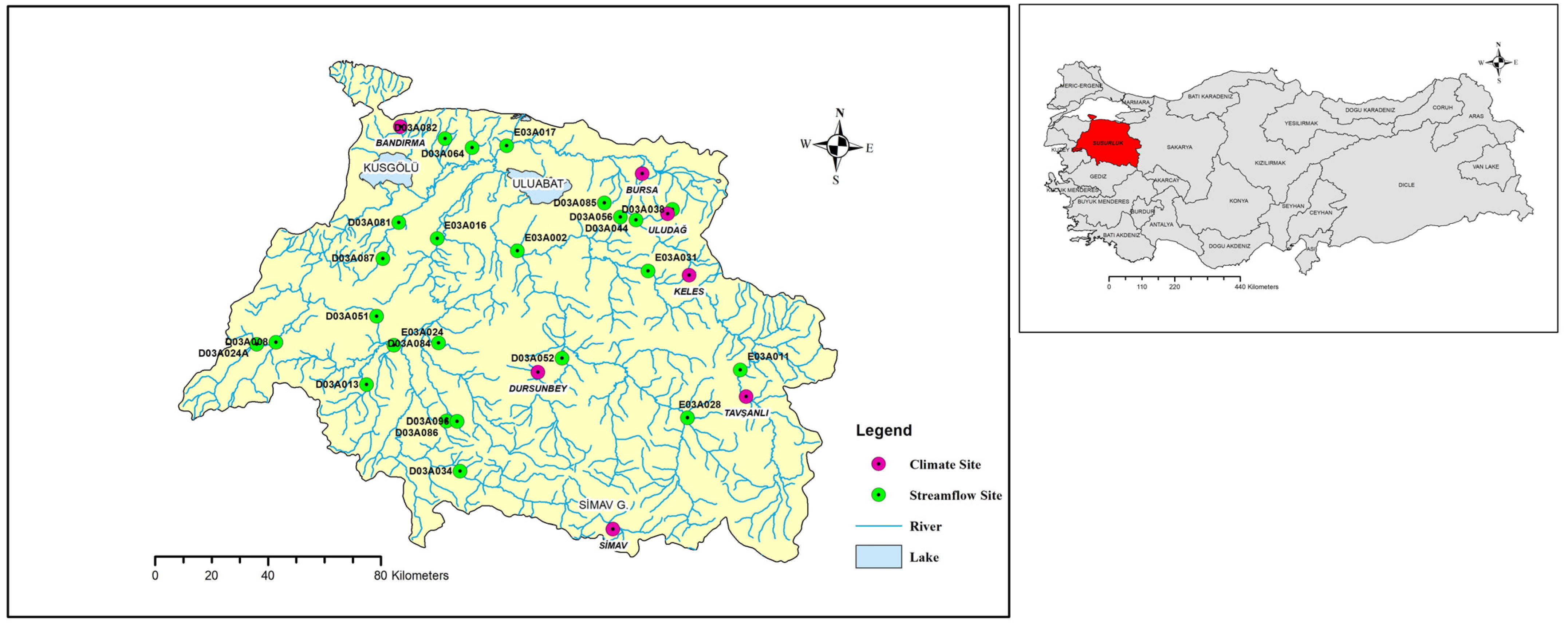
2.1. Study Area and Data Set

The Susurluk Basin, located in western Turkey, was chosen as the study area. The Susurluk Basin is located between 39–40° North latitudes and 27–30° East longitudes. The location of the Susurluk Basin is approximately 24,332 km2, corresponding to 3.11% of Turkey’s area. The total precipitation area of the basin is approximately 22,399 km2, and its annual average flow is 5.43 km3 [44]. The location of the Susurluk Basin in Turkey and the streamflow and climate observation sites in the Susurluk Basin are shown in Figure 1.
Every streamflow observation site in the Susurluk Basin underwent a thorough evaluation in terms of daily data availability. To ensure the most reliable and consistent estimates in our analysis, we selected twenty-four streamflow observation sites with data spanning 25 years or more operated by General Directorate of State Hydraulic Works, Ankara, Turkey. These sites were strategically located on nonregulated creeks, a deliberate choice to avoid any anthropogenic consequences of water utilization and management. For a comprehensive overview, please refer to Table 1 for detailed information about the streamflow observation sites used in the study and Table 2 for the seven climate observation sites where monthly precipitation data were obtained.

2.2. Methods

2.2.1. Brief Methodology

The methods applied for the study were briefly given below:
  • First, daily streamflow time series were obtained from streamflow observation sites in the Susurluk Basin.
  • 7-day, 15-day, 30-day, and 60-day low-flow time series were calculated using daily flow time series to reflect the demand for water resources. Low-flow rates are annual minimum d-day average flows.
  • With the help of geographic information systems (GIS), the physical, morphological, and hydrological characteristics of the Susurluk Basin were calculated, and the watersheds were delineated.
  • To check whether the data are suitable for statistical analysis, the discordancy measure (Di) was first applied to the data, and discordant sites were determined. Frequency distributions were applied to the d-day low-flow time series of each year. After parameter estimation and a test of goodness-of-fit with distributions, d-day low-flows between the basin’s physical, morphological, and hydrological features at different probability levels (risk) and return periods were estimated at the site.
  • Various frequency distribution functions such as Exponential (EXP), 2-parameter exponential (EXP2), Frechet (FRE), 3-parameter Frechet (FRE3), Gamma (G), 3-parameter gamma (G3), Generalized extreme values (GEVs), Generalized gamma (GG), 4-parameter generalized gamma (GG4), Generalized logistic (GLO), Generalized Pareto (GPA), Logarithmic logistic (LLO), 3-parameter logarithmic logistic (LLO3), 3-parameter logarithmic Pearson (LP3), Logistic (LO), Logarithmic normal (LN), 3-parameter logarithmic normal (LN3), Normal (N), Weibull (WE), 3-parameter Weibull (WE3) were used for the estimation of at-site quantities.
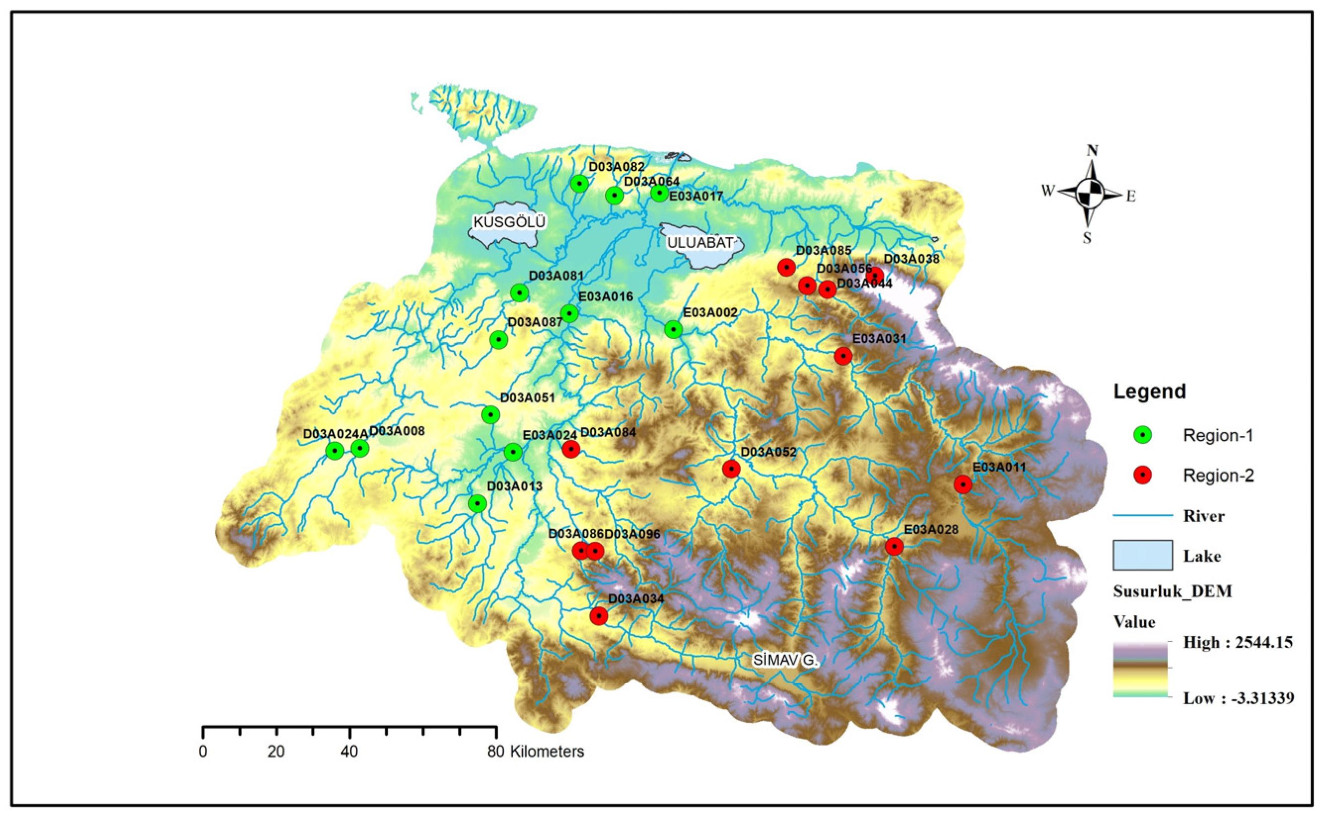
  • Before regionalization, cluster analysis (CA) and principal component analysis (PCA) were performed on group sites to identify homogeneous regions. To determine whether the regions are homogeneous, the discordancy, heterogeneity test, and goodness-of-fit measure tests for each homogeneous region provided were determined with the L-moment approach, and frequency analysis was performed.
  • For each homogeneous region obtained, regional models indicating the relationship between d-day low flows and the basin’s physical, morphological, and hydrological characteristics were developed using ordinary univariate and multivariate linear or univariate non-linear regression and principal component regression analyses [44].

2.2.2. Determination of Watershed Physiographic Parameters

Determining the physiographic features based on the basin is very important in understanding the drainage characteristics. These features can be used to develop rainfall–runoff models, obtain flow duration curves, apply regional models, and analyze floods and droughts. The correct interpretation of the physiographic features, together with the hydrological variables, helps to determine the hydrological characteristics of the basin correctly. First, a hydrological analysis must be performed in the study area to determine the physiographic features. The geographic information system ArcGIS Desktop 10.8 and ArcHydroTools (10.8.0.34) softwares were used to determine the physiographic features of the Susurluk Basin, and a digital elevation model (DEM) with a resolution of 10 × 10 m was used, as shown in Figure 2. After the hydrological analysis study was completed, catchments were determined separately for 24 streamflow observation sites used within the scope of the study, and physiographic characteristics were determined for each catchment. The Thiessen polygon method was applied to calculate the average annual precipitation amount of the catchment [44].

2.2.3. Data Completion

There are many methods for completing the deficiencies in the data sets. Within the scope of this study, correlation analysis was performed first between the streamflow data sets. Then, among the data sets with the highest correlation, the monthly averages were multiplied by the available data, and the completed data sets were obtained. The “Python–Spyder 5.1.5” application was used for data completion [44].

2.2.4. Detection of Annual Minimum d-Day Low Flows

D-daily or d-monthly flows can be used in low-flow analysis. However, n-daily flow rates are generally used in drought analyses and studies of river hydrology. It should be noted that 7-day low flows are mostly used in drought studies. ((Q1 + Q2 + … + Qn)/n), ((Q2 + Q3 + … + Qn+1)/n), …, ((Qm + Qm+1 + … + Qm+n−1)/n) process steps are repeated sequentially, and the data set is created [13].

2.2.5. At-Site Frequency Analysis

At-site frequency analysis is the statistical method that gives the lowest average flow over the d-day period with a y-year recurrence period for each site. It helps determine the low flow regime of the basin. Qd,y denotes it. For example, the most common low flow index corresponding to a 7-day, 10-year recurrence period is Q7days, 10years. Other low-flow indexes, such as the Q7,2, Q30,10, and Q30,2, also are used [45]. In Canada, Q30,5 is a common index [5]. Ref. [13] introduces the Q15;7 and Q60;2 as new indexes for 15- and 60-day low flows in addition to the common Q7,10 and Q30,5 low-flow indexes for the Tigris and Euphrates basins, and they state that these new indexes are useful for medium- and long-term requirements in the region and beyond, such as industrial and agricultural needs, as well as the environmental flow of downstream rivers.
Low flow indexes of Q7days,10years, Q15days,7years, Q30days,5years, and Q60days,2years are frequently preferred within the scope of hydrological studies since they reflect hydrological studies better. In this study, various frequency distribution functions (see Section 2.2.1) for at-site frequency analysis were used, and the Kolmogorov–Smirnov test was applied as a goodness-of-fit test.

2.2.6. Regional Analysis

L-Moments and L-Moment Ratios

In this study, the L-moment approach was applied to low-flow indexes to determine discordancy and heterogeneity measures and the probability distributions that provide the best fit to hydrologically homogeneous regions [46].
The L-moment approach, with its precision in expressing linear functions calculated by the probability-weighted moments method, can accurately reveal the character of hydrological data and determine the shape of probability distributions. It also provides precise information about a distribution’s location, scale, and shape. Probability-weighted moments are obtained with the help of Equation (1), where X represents the statistical data and F (X) represents the cumulative distribution function of X.
Mp,r,s = E [Xp{F (X)}r{1 − F (X)}s]
The probability-weighted moment βr is used if the data are an increasing sequence, and in Equation (2), the probability-weighted moment βr is equal to the multiplication of the data X by the powers (r) of the cumulative distribution function F (X). Here, the F (X) function represents the probability function in which X is given different weights for different r values.
βr = E [X {F (X)} r]      r = 0, 1, 2, …
After the probability-weighted moments are obtained, the first four sample L-moments, denoted by r (r = 1, 2, …), are given as a linear combination in Equation (3).
1 = b 0 , 2 = 2 b 1 b 0 , 3 = 6 b 2 6 b 1 + b 0 , 4 = 20 b 3 30 b 2 + 12 b 1 b 0 ,
Then, dimensionless sample L-moment ratios (t) are expressed as in Equation (4) with the help of L-moments of 1 and 2 , and higher order 3 and 4 ;
t = 2 / 1   ( L-coefficient of variation , L-Cv ) t 3 = 3 / 2   ( L-skewness , L-Cs ) t 4 = 4 / 2   ( L-kurtosis , L-Ck )
Two-parameter or three-parameter distribution functions can be used in low-flow calculations, and the L-moment method, which gives less bias compared to ordinary product moments and maximum likelihood methods, can be considered a useful and reliable method in calculating the values of distribution functions.

Discordancy Measure (Di)

The discordancy measure is applied to detect completely discordant sites in a proposed group. In this context, when determining discordant sites, the L-moment values of that site are used. In the case of discordant sites, the site is first either completely removed from the data set or outlier values are detected in the data set, and the data set is updated and re-analyzed. If any site appears completely out of order, it may be possible to shift that site to another area. The discordancy measure is the determination of the discordant sites within a region, which is explained by [47] as in Equations (5)–(7).
u ¯ = N 1 i = 1 N u i
K = i = 1 N ( u i u ¯ ) ( u i u ¯ ) T
D i = 1 3 N ( u i u ¯ ) T K 1 ( u i u ¯ )
where ui is the vector of L-moment ratios of site i, K is the covariance matrix of this vector, and u ¯ is the mean of the vector. For a site to be considered discordant, the discordancy measure must be greater than the critical table value of 3.0, which varies depending on the number of sites in the region [47].

Basin Classification

The cluster analysis (CA) classification method was used. The heterogeneity measure was applied to the regions obtained due to the clustering, and a dendrogram was obtained as a tree graph in which the areas were separated. CA is a collection of methods that help divide units, variables, or units and variables whose natural groupings are not known precisely into subgroups similar to each other in the X data matrix. Ward’s connection method (Equation (8)), one of the hierarchical clustering methods, was used, and the Euclidean square distance measure (Equation (9)) was used to determine the similarities between units. Average streamflow discharges for all years were used to reflect the at-site characteristics and hydrological and physiographic attributes of the basin for cluster vectors [48].
d m j = ( N j + N k ) d k j + ( N j + N l ) d l j N j d k l N j + N m
The symbols Nj, Nk, Nl, and Nm represent the numbers of observations in clusters j, k, l, and m.
d ( i , k ) = j ( x i j x k j ) 2
where d (i, k) indicates the distance between observations i and k. Small values of d (i, k) suggest that the basins exhibit more similar site attributes.

Heterogeneity Measure (H)

After specifying a suitable region according to the discordancy measure, the heterogeneity measure was applied to evaluate whether the region was homogeneous. Heterogeneity measure: It was calculated for three different L-statistics: L-coefficient of variation and H1, L-coefficient of variation and combination of L-skewness ratios, H2, and combination of L-kurtosis and L-skewness ratios, and H3. From here, the H statistic for all three cases is written as in Equation (10).
H = V o b s μ v σ v
where Vobs is the weighted standard deviation obtained from the regional data according to the L-moment ratios μv and σv. It shows the mean and standard deviation of the number of simulations of the Vobs statistics. This study used the four-parameter Kappa probability distribution, which is strong while performing the simulation since it represents many distributions in the frequency analysis of extreme hydrological events. According to this test, if H < 1, the region is considered acceptably homogeneous; if 1 ≤ H < 2, it is probably heterogeneous and if H ≥ 2, it is heterogeneous. A negative H value indicates that the separation between the at-site sample L-coefficient of variation values is greater than expected. If the H value is lower than −2, it suggests too many cross-correlations between sites and excessive discordancy [49].

The Goodness-of-Fit Measure (ZDIST)

In regional frequency analyses, a single probability distribution best fits the data obtained from sites in the selected homogeneous region. A method called the ZDIST statistic has been proposed for the fit criterion given in Equation (11), and depending on the L-kurtosis ratio and any probability distribution,
Z D I S T = ( τ 4 D I S T t 4 R + B 4 ) / σ 4
In Equation (9), t 4 R represents the regional average L-kurtosis ratio of the sample in B 4 and   σ 4 , respectively, the bias value and standard deviation of the regional average L-kurtosis ratio, and is expressed in Equations (12) and (13), respectively,
B 4 = N s i m 1 m = 1 N s i m ( t 4 ( m ) t 4 R )
σ 4 = [ ( N s i m 1 ) 1 { m = 1 N s i m ( t 4 ( m ) t 4 R ) 2 N s i m B 4 2 } ] 0.5
In Equations (12) and (13), Nsim refers to the number of simulations performed with the help of Kappa distribution, and m refers to the number of simulated regions. Simulations were carried out using the Monte Carlo technique. The three parameters, Generalized logistic, Generalized extreme values, Generalized normal, Pearson type 3, and Generalized Pareto distributions, were used in this study for regional analysis. If the absolute ZDIST ≤ 1.64 in any distribution, this distribution is considered suitable for regional distribution. However, among the distributions considered, the one that provides the absolute value closest to zero is selected as the most appropriate.

2.2.7. Principal Component Analysis (PCA)

PCA analysis is applied to reduce dimensions (reduce the number of variables), eliminate the relationship structure between variables, and prepare data for other statistical analyses. In PCA analysis, linear combinations of variables related to each other can be determined, and there must be a relationship between the variables defined in the initial system [50]. Although it is not possible for all correlations between variables to be zero, correlations very close to zero mean that the similarity of the principal components to the initial variables increases. The covariance matrix for the random variable vector X: px1 is Cov (X)= , and the eigenvalues of this matrix are as follows:
|Σ − λIp| = 0
The roots of Equation (14) are the λj of the form λ1 > λ2 >⋯>λp > 0. The principal components are written as linear functions of the original or standard variables. So, the basic components are as follows:
Y1 = t1X = t11 X1 + t21 X2 + ⋯ + tp1 Xp
Y2 = t2X = t12 X1 + t22 X2 + ⋯ + tp2 Xp
Yp = tpX = t1p X1 + t2p X2 + ⋯ + tpp Xp
Variances and covariances can be calculated for each principal component. Here, the variance for the principal component of Yj is calculated as given in Equation (16), and the covariance between the principal components of Yj and Yk (jk = 1, 2, …, p) is calculated as given in Equation (17).
Var (Yj) = Var (tjX) = tjVar (X) tj = tj′Σtj
Cov (Yj, Yk) = Cov (tjX, tkX) = tjCov (X) tk = tj′Σtk
Equations (18) and (19) give the total variance of the initial system and j—the variance explanation ratio (VER) of the principal component.
σ t o p 2 = i z ( Σ ) = σ 11 + + σ p p = λ 1 + + λ p
V E R = V a r ( Y j ) σ t o p 2 = λ j σ t o p 2
This study used a data set of 13 physiographic watershed (drainage basin) variables for cluster and principal component analysis. These variables: elevation (E), latitude (X), longitude (Y), watershed area (WA), watershed highest elevation (WHE), watershed lowest elevation (WLE), watershed slope (WS), long-term average flow (LAF), longest stream path (LSP), longest stream path slope (LSPS), largest stream elevation (LSE), smallest stream elevation (SSE), and long-term average precipitation (LAP) were obtained from the digital elevation model [44].

2.2.8. Development of Regional Hydrological Drought Models

The regression technique is the most commonly used approach for relating low-flow magnitudes at different return periods to a watershed’s physical and hydro-climatological characteristics. The regional drought model developed in this study is an ordinary univariate and multivariate linear or univariate non-linear regression model and principal component regression (PCR) that also includes watershed characteristics [51]. Multivariate linear regression can define watershed characteristics and low-flow index (Qd,T) for hydrologically homogeneous regions, as shown in Equation (20).
Q d , T = β 0 + β 1 X 1 + β 2 X 2 + + β n X n + ε
where β 0 intercept parameter, β1, …, βn slope parameters, X1, …, Xn is the basin characteristics, and ε: error term. If the model is established using a low-flow index and only one independent variable, it is a univariate model; if more than one independent variable is used, it is a multivariate linear regression model. Univariate non-linear models were constructed to include logarithmic, quadratic, and cubic types. A statistically significant model is selected as the best among these regression models. If more than one statistically significant regression model is found, the best model with the highest coefficient of determination (R2) is selected. R2 describes the proportion of the statistical variance in observed low flows that the regression model can explain.
On the other hand, in ordinary regression, the problem of high variance in the test set may be encountered even though it fits the model well. To minimize these problems, one can reduce the multicollinearity of a data set by using the PCR algorithm. PCR uses PCA score coefficients and then performs linear regression on these new principal components. In PCR, the principal components of the independent variables are used instead of directly regressing the dependent variable onto the independent variables. The PCR model has important advantages, such as reducing the number of features, being useful in data sets facing multicollinearity problems, being useful in data sets with highly correlated and even collinear features, and reducing the problem of overfitting. The PCR technique is unbiased because all the components used as new predictors are orthogonal. The PCR algorithm can be explained by the following Equations (21)–(23), [52,53]:
Q d , T = β 0 + β 1 ξ 1 β 2 ξ 2 + + β K ξ K        K i
Q d , T is the dependent variable (low-flow index), ξK is the Kth principal component, and i is the total number of variables. If Z variables are substituted for the X variables in the ordinary regression (Equation (20)) and the principal components are linear combinations of the original data and are defined as;
ξ 1 = l 11 Z 1 + l 21 Z 2 + + l i 1 Z i ξ 2 = l 12 Z 1 + l 22 Z 2 + + l i 2 Z i ξ K = l 1 i Z 1 + l 2 K Z 2 + + l i K Z i
Combining Equations (21) and (22) will provide a PCR equation in which independent variables replace the principal components;
Q d , T = β 0 + β 1 l 11 Z 1 + l 21 Z 2 + + l i 1 Z i + β 2 l 12 Z 1 + l 22 Z 2 + + l i 2 Z i + β K ( l 1 i Z 1 + l 2 K Z 2 + + l i K Z i )

3. Results

The hydrological analysis study determined 24 micro-drainage basins (watersheds) in the Susurluk Basin, and the physiographic and hydrological parameters of these watersheds are given in Table S1.
Daily data sets at the sites were correlated to complete the missing flow data. The data sets with the highest correlation between the sites were determined and matched with each other for data completion. The monthly average flow data were calculated separately for each data set for each month, and the data completion process was carried out by multiplying their averages with the original data. The trend graphs of the original data and the completed data are given in Figure S1.

3.1. At-Site Frequency Distribution and Relevant Low-Flow Discharges

Before developing regional low-flow frequency models in homogeneous basins, at-site frequency analysis results are given in Table S2 by applying different frequency distributions to different low-flow indexes. Table S2 shows that the most dominant distributions for low flows throughout the basin are the Generalized extreme values and Generalized Pareto distributions.

3.2. Determination of Homogeneous Regions

Within the scope of L-moment analyses, 7, 15, 30, and 60-day flow data containing the lowest flow of each year were created, and calculations were made using routines written by [54] with FORTRAN 77 source codes (L-moments, version 3.04).
The first step in finding the regional frequency distribution for low flows in the Susurluk basin is to calculate the L-moments of the low-flow indexes determined at the sites, including the L-Cv, L-Cs, and L-Ck ratios for considering the whole basin as a region. Figure 3 presents the L-moment ratio diagrams for different low-flow indexes. It is seen that the region is not homogeneous since the L-Cv and L-Cs ratios at the sites are distributed over a wide area around the weighted mean. However, discordancy measures were also calculated for low-flow indexes in the Susurluk basin to make a better decision about the level of discordancy. Table 3 provides discordancy measures for all sites and all low-flow indexes. According to Table 3, the D03A085 site is seen as discordant for 7-day and 60-day low-flows, and the E03A017 site is discordant for all low-flow indexes. At the same time, all heterogeneity measures (H1, H2, and H3 > 2) were calculated, and the results showed that the Susurluk basin, as a single region, is not a homogeneous region in terms of discordancy and heterogeneity measures. Therefore, a two-stage cluster analysis was carried out to identify areas within the basin with homogeneous characteristics. The analyses continued until the most appropriate clustering for the basin was found, using physiographic, statistical, and hydrological parameters determined specifically for the basin. According to the site locations in the dendrogram, as a result of the cluster analysis, the effect of the physiographic features of the basin is evident. The southeastern region, where the elevation is significantly higher, and the northwestern region, where the elevation is relatively lower, have formed two separate areas of the basin. However, in this case, while the results of Region-2 were homogeneous, the E03A017 site in Region-1 became a discordant site again. Suppose a discordance or heterogeneity is observed in the obtained regions. In that case, that site(s) are either completely removed from the data set or outlier values are detected in the data set, updated, and subjected to re-analysis.
The E03A017 site was not removed from the data set because it has long-term regular flow data and was highly representative as it remained downstream of the basin, and a Grubbs–Beck outlier test was applied to the E03A017 site’s data. As a result of the discordancy measure analysis applied after updating the outliers, Region-1 could finally be described as homogeneous. The locations of the sites according to the hydrologically homogeneous regions are given in Figure 4, the discordancy measures of the homogeneous Region-1 and Region-2 are shown in Table 4, and the heterogeneity measures are presented in Table 5. Table 4 and Table 5 show that all H1 and H2 values are less than 1, indicating that the proposed regions are completely homogeneous and have no discordant sites. At this study stage, regional frequency candidate distribution functions with goodness-of-fit tests were determined for each homogeneously defined low-flow region (Table 6). According to Table 6, the GNO distribution is generally the most suitable for homogeneous regions. The PE3 and GEV distributions, respectively, follow this distribution. GLO and GPA distributions were not appropriate for any low-flow data set.

3.3. Regional Hydrological Models for Ungauged Basins via Regression Approaches

PCA was performed separately for both regions before developing regional models via ordinary univariate and multivariate linear or univariate non-linear regression and principal component regression (PCR). PCA results show that the physiographic–hydrological characteristics of the selected watersheds can be divided into five principal components, which describe 97.9% and 96.4% of the variance between the selected watersheds by two regions, respectively (Table S3). However, since 12 sites were located in both regions, PCA analysis was carried out using 11 basin physiographic–hydrological characteristics by removing the longest stream path and the longest stream path slope instead of the 13 basin characteristics mentioned due to the number of variable-site discordancies in the PCA technique.
Table S3 shows the cumulative variance and the variance accounted for by each component. The VARIMAX rotation technique was used to improve PCA performance—the scree plot graphs indicate each principal component’s eigenvalues for each region in Figure S2. The importance of the first five principal components is high for both regions. Therefore, according to the scree plot graph, the first five principal components were taken as the basic components for both regions. According to the correlation between variables and component numbers, variables that are significant at the probability of p < 0.05 are shown in bold numbers in Table S4.
According to Tables S3a and S4a, for Region-1, it is seen that the highest weight in the first component is the watershed area, the watershed’s highest elevation, the largest stream elevation, and long-term average precipitation. These variables describe the highest variance/difference, 47.5%, between the selected watersheds. In the second component, elevation, the watershed’s lowest elevation and the smallest stream’s elevation have the highest eigenvalues. This component defines 33.0% of the variance/difference between watersheds. The third component has a single value in the long-term average flow, defining 8.9% of the variance/difference between watersheds. A single value for the fourth component is in the longitude, defining 5.2% of the highest variance/difference. For the fifth component, a single value is at a watershed slope and 3.3% of the highest variance/difference.
According to Tables S3b and S4b, for Region-2, it can be seen that the highest weight in the first component is the watershed area, the long-term average flow, and the long-term average precipitation. These variables describe the highest variance/difference of 40.5% between the selected watersheds. In the second component, latitude, the watershed’s lowest elevation and the smallest stream elevation have the highest eigenvalues. This component describes 21.1% of the variance/difference between watersheds. The variables with the highest eigenvalues in the third component are the watershed’s highest elevation and the largest stream elevation, which define 15.9% of the variance/difference between watersheds. As a single value for the fourth and fifth components, elevation and longitude have high eigenvalues and describe 11.1% and 7.8% of the highest variance/difference. After PCA, correlation analysis was carried out for each region separately to determine the relationship between watershed-specific physiographic and hydrological parameters and low-flow indexes. Table S5 shows all correlation coefficients, and those significant at the α: 0.05 significance level are in bold. It is seen that the highest correlation is between the elevation, latitude, watershed lowest elevation, long-term average flow, and smallest stream elevation variables for Region-1, and the highest correlation is between the watershed area, long-term average flow, the longest stream path, the longest stream path slope, and long-term average precipitation variables for Region-2 (Table S5). Regional models are developed via univariate and multivariate linear or univariate non-linear regression in two stages. The first is the ordinary univariate/multivariate regression model developed according to the correlation coefficients between basin physiographic–hydrological characteristics, and the second is the principal components regression (PCR) model using the component score coefficients in the PCA. This method has an advantage over the ordinary model with an original independent variable, such as including all data sets into regression models, possibly increasing the model accuracy as the components do not have collinearity among themselves. The parameters of each model were estimated using the ordinary least squares method and were considered significant parameters if the p < 0.05 according to the t statistics. Many trial-and-errors were made, and the search for the correct equation model continued until equations in which the R2 value was as high as possible and the probability values of all parameters assigned as independent variables (predictors) were significant at p < 0.05 were obtained.
When Q7,10, Q15,7, Q30,5, and Q60,2 are given as predictans (responses) for both regions, the developed equations of the regional ordinary univariate/multivariate regression model and principal component regression model with their average coefficients of determination (R2) and the regional model performance accuracy measures (cross-validation) (RMSE, MRE, and R2) are given in Table 7a and Table 7b, respectively.
Ordinary regression and principal component regression models were compared with root mean squared error (RMSE), mean relative error (MRE), and coefficient of determination (R2) metrics based on the jackknife procedure. In this procedure, each gauged site is considered an ungauged site, and the regional model is used to predict the low flow at that site. The RMSE measure determines the level of general agreement between the observed and estimated low flows. MRE is an error measure often used in regression problems. MRE measures the mean relative error, i.e., how much the model’s predictions differ in percentage from the ground truth. R2 defines the proportion of the statistical variance the model can express in the observed low flows [55].
In the first stage of regression models for the Q7,10 index, the first region containing near zero low-flow sites, no statistically significant (univariate or multivariate) linear relationship was obtained between Q7,10 and watershed characteristics. However, the cubic relationship was important, showing the long-term average flow as the predictor for Q7,10 in the region. In other words, the cubic non-linear relationship of the long-term average flow can be characterized by 95.64% of the base flow in the region. A statistically significant multivariate linear relationship was obtained in the second region between Q7,10 and watershed characteristics. In this region, four physiographic–hydrological features, such as watershed area, long-term average flow, the longest stream path slope, and long-term average precipitation, represented low flows by 98.92%.
The elevation, latitude, and long-term average flow predictors were the main determinants, linearly defining the 15-day minimum flows by 97.31% for the first region. In Region-2, watershed area, long-term average flow, and long-term average precipitation described 98.47% of the Q15,7 low flows.
Q30,5 was non-linearly (quadratically) related to the long-term average flow, which described 96.70% of the variation in low-flows for Region-1, whereas for Region-2, long-term average flow and long-term average precipitation predictors determined the low-flows with the watershed area as a multivariate linear relationship with a rate of 98.66%.
In the case of Q60,2, latitude and long-term average flow explained the low-flow variation in Region-1 at a level of 97.20%, while in Region-2, watershed area, long-term average flow, and long-term average precipitation variables were determined as the main predictors at a level of 98.90% to estimate longer duration minimum flows.
When cross-validation results were examined to evaluate the performance of ordinary regression models, it was shown that regression models had a small amount of lower accuracy if the gauged site was considered an ungauged site. This is explained by the fact that the average R2 percentages decrease by approximately 2–3% for each index after the cross-validation procedure. However, the MRE criterion slightly underestimates and overestimates the low flows in homogeneous regions of ordinary regression models. This deviation was lower in the 1st region estimates of 7-day, 30-day, and 60-day low flows and slightly higher in the 2nd region estimates. There is a somewhat higher deviation in the estimation of 15-day low flows. In addition, the RMSE criterion showed that the accuracy of the estimations was quite good in terms of being close to zero (Table 7a).
In the second stage, PCR models were developed to test whether more precise results could be obtained by removing collinearity from the predictors and how the combination of predictors could identify low flows in the Susurluk River basin. Using the principal components in PCA, principal component scores were calculated for sites in each region, and various PCR models were developed. The second (PC2) and third (PC3) components were effective at 83.97% for Q7,10, with low flows near zero in Region-1, the lowland plain part of the Susurluk Basin.
These two components express the importance of the elevation, watershed smallest elevation, smallest stream elevation, and long-term average flows in low-flows near zero. For Q7,10 index predictions, it was determined that the first (PC1) and second (PC2) components were effective at 95.01% in Region 2, which is the highland mountainous region of the basin. However, minimum flows can be estimated by squaring the determined equation. The watershed area, long-term average flow, long-term average precipitation, latitude, watershed largest elevation, and smallest stream elevation were found to be important in estimating Q7,10 minimum flows.
While Q15,7 low-flows were estimated, the second (PC2), third (PC3), and fifth (PC5) components showed a weight of 89.70% in the low-elevation first region of the basin. The elevation, watershed lowest elevation, smallest stream elevation, long-term average flow, and watershed slope factors affected the estimation of these flows.
The 30-day minimum flows, which are longer-term low-flows, were affected by many components, such as the first (PC1), second (PC2), third (PC3), and fifth (PC5) factors at a level of 93.71%, unlike other low-flows in the first regions. In the second region, as in other low-flow indexes, Q7,10 and Q15,7, the first and second components were explanatory with 94.74% accuracy for 30-day flows. Similarly, in other second regions, the square of the equation calculates the flow estimates.
In estimating the Q60,2 index, which is the longest-term low-flows used in this study, the second component was found to be negative, and the third component was positive at an accuracy level of 84.83% in Region-1. The first and second components contributed positively and negatively, respectively, at 94.40% in Region-2.
When evaluating the performance of principal component regression models, cross-validation results showed that principal component regression models had slightly lower accuracy in other indexes, except for the mountainous Region-2 60-day low-flow estimations, relative to the average R2, if the gauged site was considered an ungauged site. This is explained by the fact that the average R2 percentages, excluding the Region-2 60-day low-flow estimations, decrease by approximately 2–3% for other indexes after the cross-validation procedure. This situation is important for the study, as in ordinary regression models, and it is stated that the models established by using the principal components created as a combination of basin physiographic and hydrological features are quite effective and can be used for hydrological drought estimations. However, according to the MRE criterion, it is seen that the principal component regression models overestimate the low flows in homogeneous regions for all indexes in the lowland first region and estimate almost unbiasedly in the mountainous second region. On the other hand, the RMSE criterion gave very good results with reasonable values (Table 7b).

4. Discussion

In this study, at-site and regional frequency distributions were estimated using Q7,10, Q15,7, Q30,5, and Q60,2 low-flow indexes, which are important in terms of hydrological drought in the Susurluk Basin, and regional hydrological drought risk models were developed using ordinary and principal component regression techniques.
At-site frequency analyses of the study results showed that the most dominant distributions for low-flow risk and probability throughout the basin are the 3-parameter Generalized extreme values (GEVs) and Generalized Pareto (GPA) distributions, which fit hydrological extreme events. Different studies have reported that both distributions are suitable for low flows [56,57]. Typical hierarchical cluster analysis showed that using only physiographic features to classify and group basins alone is not appropriate. Therefore, physiographic, hydrological, and statistical vectors were combined to define the groups. Thus, two-stage clustering showed an advantage over simple clustering. The regions obtained with the new approach were homogeneous and free of discordant sites. Ref. [58] emphasized the importance of the two-stage cluster in their study. Regional frequency analysis of low flows showed that the GNO distribution is generally the best fit for homogeneous regions. The PE3 and GEV distributions, respectively, follow this distribution. However, an interesting result was that the GLO and GPA distributions were unsuitable for any low-flow data set. This showed that it would only sometimes be compatible with the results of at-site frequency analysis. Ref. [59] obtained similar results. However, regional frequency analysis is superior to at-site frequency analysis, even if the regions are heterogeneous.
The principal component variables obtained for estimating regional drought risk models describe the differences between watersheds and indicate the best variables for spatial analysis of low-flow characteristics in the Susurluk Basin. Linear and non-linear regression models were developed to predict ungauged basins with ordinary and principal component regression techniques. Physiographic–hydrological variables selected as independent predictors for low-flow indexes described low-flow in watersheds relatively well according to different criteria. Regression models also revealed some non-linear relationships between watershed characteristics and low-flow indexes.
According to the ordinary regression model, the long-term average flow affected the 7-day low-flows negatively from the first and third powers and positively from the second power in Region-1. Additionally, 7-day low flows increase as the second region’s watershed area and long-term average flow decrease. As the longest stream path slope and long-term average precipitation increase, 7-day low flows increase. Elevation, latitude, and long-term average flow predictors can cause 15-day low flows to increase in the stream bed in the first region. As the watershed area and long-term average flow decrease, 15-day low flows increase; as long-term average precipitation increases, 15-day low flows increase for the second region. The long-term average flow 30-day low-flows were affected positively by the first power and negatively by the second power in the first region. In the second region, as the watershed area and long-term average flow decrease, 30-day low-flows increase, and as long-term average precipitation increases, 30-day low-flows increase. In the first region, latitude and long-term average flows can cause 60-day low flows to increase in the stream bed.
In contrast, in the second region, watershed area and long-term average flows can decrease 60-day flows, and long-term average precipitation can increase them. In summary, in the high-elevation mountainous second region, the length and slope of the stream bed and the annual average precipitation parameters can significantly impact all low-flow indexes. In the first region, which has a low-elevation plain, low flows can generally be compatible with the average flows in the stream. This situation is important for the study and indicates that the models established using basin physiographic and hydrological features are quite effective and can be used to estimate regional hydrological drought detection. Ref. [60] argues that regional estimations obtained with basin characteristics are more effective.
According to the principal component regression model, the elevation, the watershed’s smallest elevation, and the smallest stream elevation negatively affected the estimation of the Q7,10 index. In contrast, long-term average flows positively affected the analysis of the Q7,10 index. The watershed area, long-term average flow, and long-term average precipitation positively affected the prediction of the shortest-term minimum flows in Region-2. In contrast, latitude, watershed largest elevation, and smallest stream elevation negatively affected the mountainous part of the Susurluk Basin for the second region. The second component negatively affected the prediction of Q15,7 flows, while the third and fifth components had a positive effect. In mountainous Region-2, an equation consisting of the first and second components was obtained, similar to Q7,10. However, it is seen that Q15,7 low-flow discharges can be estimated by squaring this equation. In the 15-day low-flow estimation equation in Region-2, while the first component parameters, watershed area, long-term average flow, and long-term average precipitation, were positive, the second component parameters, latitude, watershed lowest elevation, and smallest stream elevation, were negatively included. A larger number of watershed physiographic–hydrological characteristics explain 30-day low flows. These characteristics in the second component express the 30-day flows in a negative direction, while the attributes in the other first, third, and fifth components express them positively. The longest-term low flows, the 60-day flows used in this study, were negatively and positively affected by the first, second, and third component parameters.
The Susurluk River flows into the Marmara River, an inland sea in Turkey. The length of the Susurluk River and its tributaries is short, depending on the landforms, and their basins are narrow. The Susurluk River is formed by the merger of Kocaçay, coming from Kuş (Bird) Lake, and Mustafa Kemalpaşa and Nilüfer streams, coming from Ulubat Lake, located in the downstream parts of the basin. The Susurluk River collects most of the waters of Southern Marmara. Therefore, it can be said that the natural Kuş (Bird) Lake and Ulubat Lake, located at the downstream and outlet points of the basin, positively affect streamflow discharges. This situation is especially effective in the northern and northwestern parts of the first region [44].
On the other hand, 23 dams/ponds on the Susurluk River tributaries cause pressure by regulating water resources, and eight hydroelectric power plants are used for agricultural, urban, or industrial purposes. Water withdrawals can alter water flow and sediment movements and have significant consequences downstream and at the river mouth. Additionally, regulating the hydraulic regime changes the natural regime of the river by increasing flows in the summer and decreasing flows in the winter. However, the study used streamflow data from flow observation sites upstream of these hydraulic structures whenever possible. However, these structures significantly reduce the flow rate by regulating the stream [43].
The performance of the ordinary regression technique was increased by adding factor scores to the principal component regression technique. However, according to the coefficient of determination (R2), the PCR model can only improve the ordinary regression performance for some indexes. The accuracy level of the ordinary regression technique is higher than that of the principal component regression in all indexes and regions. However, although it may seem like this, the MRE cross-validation criteria in the PCR model showed that the model estimations were quite strong, especially in the mountainous second region for all indexes, and it was determined that the ordinary regression made stronger estimations in all other indexes except 15-day low flows in the lowland first region. Therefore, ordinary and principal component regression regional models are relatively better than at-site models and can be applied to estimate ungauged catchments for short-, medium-, and long-term low flows. Ref. [61] states that regional estimates are superior to at-site estimates for unmeasured basins.
Furthermore, cross-validation showed that it is necessary to consider other watershed characteristics, such as vegetation and land use types, geological formations, and soil types, to regionalize low flow. This explains hydrological drought better than the existing features used in this study. Additionally, two advantages of this research are that it uses the most common low-flow indexes, presents a new set of low-flow indexes for regional agricultural water resources management for the Susurluk Basin (Q15,7 and Q60,2), and is the first time regional low-flow analyses are calculated for the basin. These low-flow studies are very useful and critical for further water resources management, especially state water resources planning in Turkey. Another important advantage of this study is the combination of regional L-moment algorithms, two-stage cluster analysis, and different regression techniques for estimating regional hydrological drought in ungauged basins. Ref. [62] performed low flow analysis with more than one method and advocated the mixed probability distribution approach.

5. Conclusions

Low-flow frequency analysis studies are important in taking measures that can reduce the negative effects of dry periods. Susurluk Basin is among the basins that can be highly affected by drought risk due to its agricultural, economic, and natural resources. Problems such as decreasing water resources in the basin, increasing water demand due to increasing population, and more frequent and severe drought disasters due to climate change may pose major problems in ensuring sustainable water management. In this study, regional hydrological drought models were developed for water supply systems in the Susurluk Basin. Regional models were performed with ordinary and principal component regression techniques using regional low-flow frequency analysis with L-moment approaches, and the physical and hydrological characteristics of watersheds were identified as important.
Our study’s findings, the first of their kind for the Susurluk Basin, hold significant implications for water management in the region. The results, which reveal the effectiveness of ordinary regression models in the lowland first region and the suitability of principal component regression models for the mountainous second region, can revolutionize our approach to managing hydrological drought in these areas.
The approaches proposed in this study have been applied for the first time to the Susurluk Basin, and the results obtained can be improved and applied to other basins affected by drought. In future studies, using different empirical hydrological drought indexes and considering seasonal low-flows and their probabilities and relationships with watershed characteristics is highly recommended to paint a better picture of hydrological drought in the Susurluk Basin. Finally, the main limitation of this research is anthropogenic effects and intense water withdrawal from wells in the basin, which prevents the use of a larger and more extensive database. We also suggest that investigating human impact and climate change on hydrological drought should be analyzed in a non-stationary way.

Supplementary Materials

The following supporting information can be downloaded at: https://www.mdpi.com/article/10.3390/w16111473/s1, Figure S1: Trend graphs of the original and the completed data; Figure S2: The scree plot graphs of the principal component analysis for Region-1 (a) and Region-2 (b); Table S1: Physiographic and hydrological parameters of 24 micro-drainage basins (watersheds); Table S2: At-site frequency analysis and relevant return period discharges for different low-flow index; Table S3: Eigenvalue, variance, and cumulative variance values for each component for Region-1 (a) and Region-2 (b); Table S4: Eigenvalues for each physiographic, hydrological, and meteorological variable and principal component (PC) for Region-1 (a) and Region-2 (b); Table S5: Pearson product correlation coefficients between watershed physiographic and hydrological characteristics and low flow indexes according to homogeneous Region-1 (a) and Region-2 (b).

Author Contributions

Conceptualization, Ç.G. and A.S.A.; methodology, Ç.G., A.S.A. and H.E.P.; software, Ç.G., A.S.A. and H.E.P.; validation, Ç.G., A.S.A. and H.E.P.; formal analysis, Ç.G. and A.S.A.; investigation, Ç.G. and A.S.A.; resources, Ç.G. and A.S.A.; data curation, Ç.G. and A.S.A.; writing—original draft preparation, Ç.G. and A.S.A.; writing—review and editing, A.S.A. and H.E.P.; visualization, Ç.G.; supervision, A.S.A. All authors have read and agreed to the published version of the manuscript.

Funding

This research received no external funding.

Data Availability Statement

Restrictions apply to the availability of these data. Data were obtained from a third party and are available from the authors with the permission of a third party.

Acknowledgments

This work was prepared from the M.Sc. thesis of Çiğdem Gürler under the supervision of Alper Serdar Anli. We also thank the General Directorate of State Hydraulic Works (DSI) for providing daily flow data.

Conflicts of Interest

The authors declare no conflicts of interest.

References

  1. UNCCD. Zero Net Land Degradation, A Sustainable Development Goal for Rio+20 to Secure the Contribution of Our Planet’s Land and Soil to Sustainable Development, Including Foodsecurity and Poverty Eradication, Bonn. 2012. Available online: https://catalogue.unccd.int/58_Zero_Net_Land_Degradation.pdf (accessed on 19 May 2024).
  2. Köken, E. Regionalization of Tigris Basin Low Flow Characteristics. Master’s Thesis, Dokuz Eylül University, İzmir, Türkiye, 2009. (In Turkish). [Google Scholar]
  3. Yıldırımlar, O. Analysis of Low Flows in the Euphrates Basin. Master’s Thesis, Istanbul Technical University, Sarıyer/İstanbul, Türkiye, 2012. (In Turkish). [Google Scholar]
  4. Bayazit, M.; Onoz, B. Flood and Drought Hydrology; Nobel Publications: Istanbul, Turkey, 2008; 259p. (In Turkish) [Google Scholar]
  5. Ouarda, T.B.M.J.; Charron, C.; St-Hilaire, A. Statistical models and the estimation of low flows. Can. Water Resour. J. 2008, 33, 195–206. [Google Scholar] [CrossRef]
  6. Ouarda, T.B.M.J. Handbook of Applied Hydrology, 2nd ed.; Chapter 77, Regional Flood Frequency Modeling; McGraw-Hill Education: New York, NY, USA, 2017. [Google Scholar]
  7. Gustard, A.; Bullock, A.; Dixon, J.M. Low Flow Estimation in the United Kingdom; IH Report No.108; Institute of Hydrology: Wallingford, UK, 1992; 88p. [Google Scholar]
  8. Laaha, G.; Bloschl, G. A comparison of low flow regionalization methods–catchment grouping. J. Hydrol. 2006, 323, 193–214. [Google Scholar] [CrossRef]
  9. Engeland, K.; Hisdal, H. A comparison of low flow estimates in ungauged catchments using regional regression and the HBV-model. Water Resour. Manag. 2009, 23, 2567–2586. [Google Scholar] [CrossRef]
  10. Mamuna, A.A.; Hashim, A.; Daoud, J.I. Regionalisation of low flow frequency curves for the Peninsular Malaysia. J. Hydrol. 2010, 381, 174–180. [Google Scholar] [CrossRef]
  11. Ahn, K.; Merwade, V. The effect of land cover change on duration and severity of high and low flows. Hydrol. Process. 2017, 31, 133–149. [Google Scholar] [CrossRef]
  12. Cammalleri, C.; Vogt, J.; Salamon, P. Development of an operational low-flow index for hydrological drought monitoring over Europe. Hydrolog. Sci. J. 2017, 62, 346–358. [Google Scholar] [CrossRef]
  13. Anli, A.S.; Modarres, R.; Apaydin, H. A Hybrid Approach for Regional Low-Flow Frequency Analysis for the Upper Tigris and Euphrates Basin. J. Hydrol. Eng. 2023, 28, 04023015. [Google Scholar] [CrossRef]
  14. Institute of Hydrology. Low Flow Studies; Report No.1 Research Report, (Low Flow Studies 1); Institute of Hydrology: Wallingford, UK, 1980; 55p. [Google Scholar]
  15. Nathan, R.J.; McMahon, T.A. Overview of a Systems Approach to the Prediction of Low Flow Characteristics in Ungauged Catchments. In National Conference Publication; Institution of Engineers, Australia: Barton, Australia, 1991; Volume 1, pp. 187–192. [Google Scholar]
  16. Nathan, R.J.; McMahon, T.A. Estimating low flow characteristics in ungauged catchments. Water Resour. Manag. 1992, 6, 85–100. [Google Scholar] [CrossRef]
  17. Smakhtin, V. Low flow hydrology: A review. J. Hydrol. 2001, 240, 147–186. [Google Scholar] [CrossRef]
  18. Arbelaez, A.C.; Castro, L.M. Low Flow Discharges Regional Analysis using Wakeby Distribution in an ungauged basin in Colombia. In AGU Hydrology Days; Colorado State University: Fort Collins, CO, USA, 2007. [Google Scholar]
  19. Castiglioni, S.; Castellarin, A.; Montanari, A. Prediction of low-flow indices in ungauged basins through physiographical space-based interpolation. J. Hydrol. 2009, 378, 272–280. [Google Scholar] [CrossRef]
  20. Kirkby, M.; Gallart, F.; Kjeldsen, T.; Irvine, B.; Froebrich, J.; Lo Porto, A.; De Girolamo, A. Classifying low flow hydrological regimes at a regional scale. Hydrol. Earth Syst. Sci. 2011, 15, 3741–3750. [Google Scholar] [CrossRef]
  21. Grandry, M.; Gailliez, S.; Sohier, C.; Verstraete, A.; Degre, A. A method for low-flow estimation at ungauged sites: A case study in Wallonia (Belgium). Hydrol. Earth Syst. Sci. 2013, 17, 1319–1330. [Google Scholar] [CrossRef]
  22. Sharma, S.; Gajbhiye, S.; Tignath, S. Application of principal component analysis in grouping geomorphic parameters of a watershed for hydrological modeling. Appl. Water Sci. 2015, 5, 89–96. [Google Scholar] [CrossRef]
  23. Van Lanen, H.A.; Wanders, N.; Tallaksen, L.M.; Van Loon, A.F. Hydrological drought across the world: Impact of climate and physical catchment structure. Hydrol. Earth Syst. Sci. 2013, 17, 1715–1732. [Google Scholar] [CrossRef]
  24. Bulu, A.; Cokgor, S.; Cigizoglu, H. Statistical analysis of low flows on Thrace Region. In Proceedings of the UNESCO FRIEND-AMHY Conference, Thessalonique, Greece, September 1995; pp. 91–104. [Google Scholar]
  25. Onoz, B.; Bulu, A. Frequency Analysis of Low Flows in the Thrace Region. Turk. J. Civ. Eng. 1996, 93, 1243–1254. [Google Scholar]
  26. Sertbas, Y. The investigation of the most suitable probability distribution for the low flows of the Sakarya Basin River flows. Master’s Thesis, Istanbul Technical University, Sarıyer/İstanbul, Türkiye, 1996. (In Turkish). [Google Scholar]
  27. Bulu, A.; Onoz, B. Frequency analysis of low flows by the PPCC test in Turkey. UNESCO FRIEND-AMHY’97—Reg. Hydrol. Concepts Models Sustain. Water Resour. Manag. 1997, 246, 133–140. [Google Scholar]
  28. Saris, F. Low Flow Analysis in Porsuk Stream Basin. J. Geogr. 2016, 33, 72–82. (In Turkish) [Google Scholar]
  29. Durak, S. Low flow hydrology and Aegean Region application. Master’s Thesis, Istanbul Technical University, Sarıyer/İstanbul, Türkiye, 2000. (In Turkish). [Google Scholar]
  30. Saraçoğlu, Ö. Low Flow Hydrology and Its Application in the Mediterranean Region. Master’s Thesis, Istanbul Technical University, Sarıyer/İstanbul, Türkiye, 2002. (In Turkish). [Google Scholar]
  31. Yurekli, K.; Kurunc, A.; Gul, S. Frequency analysis of low flow series from Çekerek Stream Basin. J. Agric. Sci. 2005, 11, 72–77. [Google Scholar]
  32. Eris, E.; Aksoy, H.; Onoz, B.; Cetin, M.; Yuce, M.I.; Selek, B.; Aksu, H.; Burgan, H.I.; Esit, M.; Yildirim, I.; et al. Frequency analysis of low flows in intermittent and non-intermittent rivers from hydrological basins in Turkey. Water Supply 2019, 19, 30–39. [Google Scholar] [CrossRef]
  33. Anlı, A.S.; Öztürk, F. Regional frequency analysis of annual maximum precipitation measured in Ankara. GOU J. Fac. Agric. 2011, 28, 61–71. (In Turkish) [Google Scholar]
  34. Şen, O. Determination of Hydrological Homogeneous Regions of Türkiye Flow Variables. Master’s Thesis, Istanbul Technical University, Sarıyer/İstanbul, Türkiye, 2011. (In Turkish). [Google Scholar]
  35. Aksoy, H.; Çetin, M.; Önöz, B.; Yüce, M.İ.; Eriş, E.; Selek, B.; Çavuş, Y. Low Flows and Drought Analysis in Hydrological Basins. Turkish National Geodesy and Geophysics Union. Turkey National Meteorological and Hydrological Disasters Program-2015-01, 2018. (In Turkish). Available online: https://www.tujjb.org.tr/uploads/files/nationalprojects/hidrolojik-havzalarda-dusuk-akimlar-ve-kuraklik-analizi-tujjb-tumehap-2015-01-2240.pdf (accessed on 19 May 2024).
  36. Cavus, Y.; Aksoy, H. Spatial Drought Characterization for Seyhan River Basin in the Mediterranean Region of Turkey. Water 2019, 11, 1331. [Google Scholar] [CrossRef]
  37. Mersin, D.; Gulmez, A.; Safari, M.J.S.; Vaheddoost, B.; Tayfur, G. Drought assessment in the Aegean region of Turkey. Pure Appl. Geophys. 2022, 179, 3035–3053. [Google Scholar] [CrossRef]
  38. Gulmez, A.; Mersin, D.; Vaheddoost, B.; Safari, M.J.S.; Tayfur, G. A Joint Evaluation of Streamflow Drought and Standard Precipitation Indices in Aegean Region, Turkey. Pure Appl. Geophys. 2023, 180, 4319–4337. [Google Scholar] [CrossRef]
  39. Yuce, M.I.; Deger, I.H.; Esit, M. Hydrological drought analysis of Yeşilırmak Basin of Turkey by streamflow drought index (SDI) and innovative trend analysis (ITA). Theor. Appl. Climatol. 2023, 153, 1439–1462. [Google Scholar] [CrossRef]
  40. Bayer Altin, T.; Altin, B.N. Response of hydrological drought to meteorological drought in the eastern Mediterranean Basin of Turkey. J. Arid Land 2021, 13, 470–486. [Google Scholar] [CrossRef]
  41. Orta, S.; Aksoy, H. Development of Low Flow Duration-Frequency Curves by Hybrid Frequency Analysis. Water Resour. Manag. 2022, 36, 1521–1534. [Google Scholar] [CrossRef]
  42. Sarigil, G.; Cavus, Y.; Aksoy, H. Frequency curves of high and low flows in intermittent river basins for hydrological analysis and hydraulic design. Stoch Environ. Res. Risk Assess 2024, accepted. [Google Scholar] [CrossRef]
  43. Ministry of Agriculture and Forestry; General Directorate of Water Management; Department of Flood and Drought Management. Drought Management Planning of Susurluk Basin Projects; General Directorate of Water Management: Ankara, Turkey, 2023. (In Turkish) [Google Scholar]
  44. Gürler, Ç. Regional Low Flow Frequency Analysis for Water Supply Systems in Susurluk Basin. Master’s Thesis, Ankara University, Ankara, Türkiye, 2022. (In Turkish). [Google Scholar]
  45. Bhatti, S.J.; Kroll, C.N.; Vogel, R.M.R. Revisiting the probability distribution of low streamflow series in the United States. J. Hydrol. Eng. 2019, 24, 04019043. [Google Scholar] [CrossRef]
  46. Hosking, J.R.M.; Wallis, J.R. Regional Frequency Analysis: An Approach Based on L-Moments; Cambridge University Press: Cambridge, UK, 1997. [Google Scholar]
  47. Hosking, J.R.M.; Wallis, J.R. Some statistics useful in regional frequency analysis. Water Resour. Res. 1993, 29, 271–281. [Google Scholar] [CrossRef]
  48. Anli, A.S. Regional Frequency Analysis of Rainfall in Ankara Using L Moment Methods. Ph.D. Thesis, Ankara University, Ankara, Türkiye, 2009. (In Turkish). [Google Scholar]
  49. Hosking, J.R.M. The four-parameter kappa distribution. IBM J. Res. Dev. 1994, 38, 251–258. [Google Scholar] [CrossRef]
  50. Bulut, H. Multivariate Statistical Methods with R Applications; Multivariate Statistics II Lecture Notes; Academic Publishing: Ankara, Turkey, 2018. (In Turkish) [Google Scholar]
  51. Montgomery, D.C.; Peck, E.A.; Vining, C.G. Introduction to Linear Regression Analysis, 5th ed.; John Wiley & Sons, Inc.: New York, NY, USA, 2012; p. 836. [Google Scholar]
  52. Eslamian, S.; Ghasemizadeh, M.; Biabanaki, M.; Talebizadeh, M. A principal component regression method for estimating low flow index. Water Res. Manag. 2010, 24, 2553–2566. [Google Scholar] [CrossRef]
  53. Susilawati, S.; Didiharyono, D. Application of Principal Component Regression in Analyzing Factors Affecting Human Development Index. J. Varian 2023, 6, 199–208. [Google Scholar] [CrossRef]
  54. Hosking, J.R.M. FORTRAN Routines for Use with the Method of L-Moments, Version 3.04; Research Report RC 20525; IBM Research Division, T.C. Watson Research Center: Yorktown Heights, NY, USA, 2005. [Google Scholar]
  55. Dawson, C.W.; Abrahart, R.J.; See, L.M. HydroTest: A webbased toolbox of evaluation metrics for the standardized assessment of hydrological forecasts. Environ. Modell. Softw. 2007, 22, 1034–1052. [Google Scholar] [CrossRef]
  56. Li, M.; Li, X.; Ao, T. Comparative Study of Regional Frequency Analysis and Traditional At-Site Hydrological Frequency Analysis. Water 2019, 11, 486. [Google Scholar] [CrossRef]
  57. Ghabelnezam, E.; Mostafazadeh, R.; Hazbavi, Z.; Huang, G. Hydrological Drought Severity in Different Return Periods in Rivers of Ardabil Province, Iran. Sustainability 2023, 15, 1993. [Google Scholar] [CrossRef]
  58. Ouarda, T.B.; Charron, C.; Hundecha, Y.; St-Hilaire, A.; Chebana, F. Introduction of the GAM model for regional low-flow frequency analysis at ungauged basins and comparison with commonly used approaches. Environ. Model. Softw. 2018, 109, 256–271. [Google Scholar] [CrossRef]
  59. Strnad, F.; Moravec, V.; Markonis, Y.; Máca, P.; Masner, J.; Stočes, M.; Hanel, M. An Index-Flood Statistical Model for Hydrological Drought Assessment. Water 2020, 12, 1213. [Google Scholar] [CrossRef]
  60. Wang, M.; Jiang, S.; Ren, L.; Xu, C.Y.; Shi, P.; Yuan, S.; Fang, X. Nonstationary flood and low flow frequency analysis in the upper reaches of Huaihe River Basin, China, using climatic variables and reservoir index as covariates. J. Hydrol. 2022, 612, 128266. [Google Scholar] [CrossRef]
  61. Requena, A.I.; Ouarda, T.B.; Chebana, F. Low-flow frequency analysis at ungauged sites based on regionally estimated streamflows. J. Hydrol. 2018, 563, 523–532. [Google Scholar] [CrossRef]
  62. Laaha, G. A mixed distribution approach for low-flow frequency analysis—Part 1: Concept, performance, and effect of seasonality. Hydrol. Earth Syst. Sci. 2023, 27, 689–701. [Google Scholar] [CrossRef]
Figure 1. The location of the Susurluk Basin in Turkey and the streamflow and climate observation sites in the Susurluk Basin.
Water 16 01473 g001
Figure 2. Digital elevation model of the Susurluk Basin.
Water 16 01473 g002
Figure 3. L-moment ratio diagrams of L-Cv versus L-Cs for the sites and different low-flow indexes (◼ shows the weighted mean of the L-Cv versus L-Cs, shows L-Cv versus L-Cs for sites).
Water 16 01473 g003
Figure 4. The locations of the sites are according to the hydrologically homogeneous regions.
Water 16 01473 g004
Table 1. Characteristics of the streamflow observation sites in the Susurluk Basin.
NoSite
Code
Site
Name
Longitude–Latitude (°)Drainage
Area (km2)
Elevation
(m)
Observation PeriodSample
Size
1D03A008Kahve27.54East39.61North7411901963–201654
2D03A013İkizcetepeler27.92East39.50North4671281964–201754
3D03A024Ayaklı27.36East39.52North1152501967–201650
4D03A034Osmanlar Köp.28.32East39.25North12662771970–201748
5D03A038Uludağ29.14East40.12North2616751972–201746
6D03A044S.Saygı Brj. Gir.29.00East40.08North3773411982–201736
7D03A051Değirmenboğazı27.95East39.71North841921980–201738
8D03A052Sinderler28.72East39.62North9652941981–201737
9D03A056Sultaniye28.94East40.09North503681982–201736
10D03A064Gölecik28.28East39.61North111271984–201734
11D03A081Mürvetler28.01East40.02North289311986–201732
12D03A082Keçiler28.18East40.30North21651986–201732
13D03A084Eyüpbükü28.23East39.65North2419451987–201731
14D03A085İnegazi28.87East40.13North153061988–201730
15D03A086Adalı28.26East39.39North663751988–201730
16D03A087Yeşilova27.96East39.90North1412501989–201729
17D03A096Okçular28.30East39.40North354051991–201727
18E03A002Döllük28.51East39.62North9617401950–201768
19E03A011Küçükilet29.86East39.12North16427951950–201768
20E03A016Yahyaköy28.17East39.98North6376321953–201765
21E03A017Akçasusurluk28.40East40.26North2021953–201765
22E03A024Balıklı28.02East39.63North244941954–201760
23E03A028Dereli29.25East39.46North11655571965–201753
24E03A031Dağgüney29.06East39.92North34933651993–201725
Table 2. Characteristics of the climate observation sites in the Susurluk Basin.
NoSite CodeSite NameElevation (m)Longitude (°)Latitude (°)
117114Bandırma5127.9940.32
217116Bursa10129.0240.23
317676Uludağ187729.1340.12
417695Keles106329.2339.91
517700Dursunbey63928.6239.58
617704Tavşanlı83329.5039.55
717748Simav80928.9839.08
Table 3. Discordancy measures (Di) for different low-flow indexes.
Site CodeLow-Flow Index
7-Day 15-Day30-Day 60-Day
D03A0080.230.460.580.84
D03A0130.080.040.080.27
D03A0240.120.200.140.26
D03A0340.630.990.890.80
D03A0380.210.280.080.20
D03A0441.702.431.020.05
D03A0510.560.071.000.63
D03A0520.110.160.170.39
D03A0560.510.240.270.30
D03A0640.811.192.370.90
D03A0810.450.690.780.84
D03A0820.781.221.490.65
D03A0840.550.460.900.26
D03A0853.50 *1.722.353.36 *
D03A0860.171.860.180.61
D03A0870.080.260.421.30
D03A0960.940.090.290.18
E03A0021.271.261.251.22
E03A0111.020.781.021.08
E03A0161.881.620.990.98
E03A0176.13 *6.04 *5.82 *5.94 *
E03A0240.440.140.100.52
E03A0280.280.330.390.38
E03A0311.551.451.422.03
Note: * Discordant site.
Table 4. Discordancy measures (Di) of different low-flow indexes for homogeneous Region-1 and Region-2.
Site CodeRegion-1Site CodeRegion-2
7-Day15-Day30-Day60-Day7-Day15-Day30-Day60-Day
D03A0080.371.791.031.79D03A0341.261.351.161.17
D03A0130.120.090.180.58D03A0380.240.440.310.57
D03A0240.330.420.260.42D03A0441.081.941.670.33
D03A0511.340.111.330.74D03A0520.150.290.340.93
D03A0640.750.881.590.63D03A0560.520.910.891.11
D03A0811.221.611.471.09D03A0841.961.281.860.62
D03A0820.921.080.980.68D03A0852.251.121.872.44
D03A0870.180.500.520.93D03A0860.461.200.260.55
E03A0020.680.680.570.59D03A0960.700.210.230.45
E03A0162.161.661.291.32E03A0110.850.700.820.84
E03A0172.742.752.732.75E03A0280.440.430.510.85
E03A0241.010.260.050.41E03A0312.082.142.072.15
Table 5. Heterogeneity measures for low-flow regions in the Susurluk basin.
Low-Flow IndexRegionNumber of SitesHeterogeneity Measure
H1H2H3
7-day112−0.1747−0.17725.5933
212−0.1811−0.17907.0201
15-day112−0.1701−0.20004.8446
212−0.2500−0.26056.7792
30-day112−0.2245−0.22355.1790
212−0.3302−0.36776.9218
60-day112−0.0520−0.05384.1992
212−0.4101−0.41585.7555
Table 6. Appropriate probability distributions according to homogeneous regions for each low-flow index.
Low-Flow IndexRegionNumber of SitesZDIST (Goodness-of-Fit Measure)
GLOGEVGNOPE3GPA
7-day1122.150.70 *0.10 **−1.50 *2.98
2122.190.77 *0.02 **−1.32 *−2.82
15-day1123.451.740.95 *−0.47 **−2.47
2122.671.19 *0.42 **−0.94 *−2.54
30-day1123.621.801.06 *−0.31 **−2.61
2122.280.67 *0.01 **−1.19 *−3.24
60-day1123.621.44 *0.78 *−0.51 **−3.66
2122.070.28 *−0.24 **−1.28 *−3.90
Notes: GLO: Generalized logistic; GEV: Generalized extreme values; GNO: Generalized normal; PE3: Pearson Type 3; and GPA: Generalized Pareto. * Appropriate distribution; ** Best-fit distribution.
Table 7. Ordinary (a) and principal component (b) regression models and their average R2 and accuracy measures for each low-flow index and each region.
Low-Flow
Index
RegionOrdinary Regression Model (a)R2p-ValueCross-Validation
RMSEMRER2
Q7,101Q7,10 = 0.2666 − 0.1192LAF + 0.01208LAF2 − 0.000091LAF395.640.00011.131.5893.53
2Q7,10 = −0.411268 − 0.0051575WA − 0.932308LAF + 0.048948LSPS + 0.396897LAP98.920.00020.167.6396.84
Q15,71Q15,7 = −100.386 + 0.0074322E + 3.55112X + 0.1835LAF97.310.00010.92−16.3195.14
2Q15,7 = −0.0188402 − 0.00505061WA − 0.927826LAF + 0.390254LAP98.470.00010.1910.9696.38
Q30,51Q30,5 = −0.4996 + 0.2636LAF − 0.000632LAF296.700.00011.190.3293.83
2Q30,5 = −0.00670212 − 0.00526292WA − 0.956042LAF + 0.404939LAP98.660.00010.199.4796.48
Q60,21Q60,2 = −65.3312 + 2.33149X + 0.21396LAF97.200.00031.11−1.3694.99
2Q60,2 = 0.0142909 − 0.0056536WA − 0.996297LAF + 0.429326LAP98.900.00010.186.2396.58
Low-Flow
Index
RegionPrincipal Component Regression Model (b)R2p-ValueCross-Validation
RMSEMRER2
Q7,101Q7,10 = 2.85024 − 2.01963PC2 + 4.77548PC383.970.00032.1729.6782.12
2Q7,10 = [0.590891 + 0.624979PC1 − 0.272818PC2]295.010.00010.15−0.3291.83
Q15,71Q15,7 = 2.98478 − 2.11063PC2 + 4.96447PC3 + 1.37115PC589.700.00031.8114.1787.69
2Q15,7 = [0.606588 + 0.63404PC1 − 0.280948PC2]294.880.00010.15−0.3291.72
Q30,51Q30,5 = 3.18191 + 1.24506PC1 − 2.2412PC2 + 5.255PC3 + 1.43846PC593.710.00021.4932.0491.58
2Q30,5 = [0.633935 + 0.645009PC1 − 0.286274PC2]294.740.00010.16−0.3591.49
Q60,21Q60,2 = 3.55864 − 2.5025PC2 + 5.87477PC384.830.00022.5919.7982.91
2Q60,2 = [0.676954 + 0.659337PC1 − 0.292911PC2]294.400.00010.17−0.3896.73
Notes: E: elevation; X: latitude; Y: longitude; WA: watershed area; WHE: watershed highest elevation; WLE: watershed lowest elevation; WS: watershed slope; LAF: long-term average flow; LSP: longest stream path; LSPS: longest stream path slope; LSE: largest stream elevation; SSE: smallest stream elevation; LAP: long-term average precipitation. PC1PC5 = Principal components 1–5.
Disclaimer/Publisher’s Note: The statements, opinions and data contained in all publications are solely those of the individual author(s) and contributor(s) and not of MDPI and/or the editor(s). MDPI and/or the editor(s) disclaim responsibility for any injury to people or property resulting from any ideas, methods, instructions or products referred to in the content.

