Article

Assessing the Effectiveness of the Use of the InVEST Annual Water Yield Model for the Rivers of Colombia: A Case Study of the Meta River Basin

by
Jhon B. Valencia
1,
Vladimir V. Guryanov
1,
Jeison Mesa-Diez
2,
Jeimar Tapasco
3 and
Artyom V. Gusarov
4,*
1
Institute of Environmental Sciences, Kazan Federal University, 420008 Kazan, Russia
2
Escuela de Estadística, Universidad del Valle, Calle 13 No. 100-00—Edificio E43, Santiago de Cali 760042, Colombia
3
Climate Action, Alliance of Bioversity International and the International Center for Tropical Agriculture (CIAT), Palmira 763537, Colombia
4
Institute of Geology and Petroleum Technologies, Kazan Federal University, 420008 Kazan, Russia
*
Author to whom correspondence should be addressed.
Water 2023, 15(8), 1617; https://doi.org/10.3390/w15081617
Submission received: 15 March 2023 / Revised: 11 April 2023 / Accepted: 19 April 2023 / Published: 21 April 2023

Abstract

:
This paper presents the results of one of the hydrological models, the InVEST “Annual Water Yield” (InVEST–AWY), applied to the Meta River basin in Colombia, which covers an area of 113,981 km². The study evaluates the performance of the model in different subbasins of the Meta River basin. The model’s accuracy was assessed using different statistical measures, including Nash–Sutcliffe Efficiency (NSE) coefficient, Root Mean Square Error (RMSE), correlation coefficients for the calibration (rcal) and validation (rval) periods. The overall performance of the model in the Meta River basin is relatively poor as indicated by the low NSE value of 0.07 and high RMSE value of 1071.61. In addition, the model explains only a 7% of the variance in the observed data. The sensitivity analysis revealed that a 30% reduction in crop coefficient (Kc) values would result in a 10.7% decrease in water yield. The model estimated, for example, the annual average water yield of the river in 2018 as 1.98 × 10¹¹ m3/year or 6273.4 m3/s, which is 1.3% lower than the reported value. The upper Meta River subbasin shows the highest NSE value (0.49), indicating a good result between observed and simulated water discharge. In contrast, the South Cravo River subbasin shows a negative NSE value of −1.29, indicating poor model performance. The Yucao River subbasin and the upper Casanare River subbasin also show lower NSE values compared to the upper Meta River subbasin, indicating less accurate model performance in these subbasins. The correlation coefficients in calibration (rcal) and validation (rval) for the upper Meta River, Yucao River, South Cravo River, and upper Casanare River subbasins were 0.79 and 0.83, 0.4 and 0.22, 0.5 and −0.25, and 0 and 0.18, respectively. These results provide useful insights into the limitations for the proper use of the InVEST–AWY model in Colombia. This study is the first to use the InVEST–AWY model on a large scale in the territory of Colombia, allowing to evaluate its effectiveness in hydrological modeling for water management.

1. Introduction

Water is vital for human activities. This resource provides ecosystem services such as water provision, purification, and regulation, which are crucial for the health and productivity of natural ecosystems, as well as for human well-being. However, as the world’s population continues to grow and the effects of climate change become more noticeable, the demand for water resources is increasing, and the availability of clean water is becoming increasingly scarce [1,2,3].
Effective planning and management of water resources require the use models to predict water yield and to understand the complex interactions between different water sources and uses [4]. However, some of the challenges in hydrology modeling are the low availability of information in remote environments, as well as the lack of knowledge of ecosystems as providers of water [5].
The Meta River basin in Colombia has an approximate area of 99,500 to 105,000 km² [6]. The river has a length of 1002 km from Guamal (upstream) to the mouth in the Orinoco River [7]. This river basin has a large percentage of areas suitable for agricultural activities [8], suggesting higher pressure on the water resources of this region in the future.
In Colombia, some studies have quantified water resources at the basin-scale level [9,10,11,12,13,14,15,16,17]. Among the limitations for water modeling in Colombia is access to hydro-climatological data in its eastern regions due to low station coverage [18].
Modeling hydrological services requires significant implementation effort and data requirements, which may not always be available [19]. For example, [16] performed one of the largest scale hydrological modeling projects in the Magdalena River basin in Colombia, which obtained good results using global and in-situ hydrometeorological information as input for multiple hydrological models.
When selecting a hydrological model, it is important to consider its capability to represent the hydrological characteristics of the region. For instance, [20] used selection scores to choose a model for the Kangsabati River basin, where they compared five conceptual models (AWBM, GR4J, HBV-light, SRM, and Sacramento) and five semi-distributed models (HEC–HMS, VIC, HFAM, HSPF, and TOPMODEL). They selected the GR4J and VIC models because they had the best performance criteria for their research zone.
Although hydrological models have different approaches to simulate the hydrological cycle, they all require input data such as rainfall, runoff, wind speed, relative humidity, soil type, catchment properties, hydrogeology, and other properties in a daily scale [20,21]. However, there are also differences between the models. The InVEST “Annual Water Yield” (InVEST–AWY) model is easy to use and requires minimum input data but may not perform well for large watersheds with low data. Nonetheless, the model can be calibrated using the Soil and Water Assessment Tool (SWAT) model outputs [22]. On the other hand, HEC-HMS is a powerful model that can handle large watersheds but requires a significant amount of input data and expertise to use effectively [23].
Furthermore, some models like Sacramento and GR4J use a lumped approach, while others like HEC-HMS and VIC use a distributed approach [20,24]. The lumped approach models are easier to use and require less input data, but they may not be suitable for large watersheds. The distributed approach models, on the other hand, are more complex and require more input data, but they can handle large watersheds and provide more accurate results [25].
Some models may require long-term series of observed hydrological and meteorological data to calibrate the model parameters, which can be difficult to obtain [24]. Models like SWAT, VIC, and GR4J may require a significant amount of input data and expertise to use effectively [23,26,27]. In areas where a reliable weather monitoring system is absent, utilizing satellite information for hydrological modeling can be a viable solution [28]. Nonetheless, the overestimation of weather variables, such as precipitation, remains a concern [28].
One of the most used models in catchment scale is the Soil and Water Assessment Tool (SWAT) [29]. However, it requires a vast amount of daily hydroclimatic information and can only be applicable in zones with good weather station data coverage. [17] used SWAT to determine water yield in northeastern Colombia, in an area with a high density of weather stations, and established the relationship between water availability, land-use change, and climate change.
Due to the high demand for information in some hydrological models [30] and the lack of hydroclimatic information in remote zones, it is necessary to explore models that require less information and computational effort but can still provide a good approximation of hydrological services assessment [31]. One such tool is the Integrated Valuation of Ecosystem Services and Tradeoffs (InVEST) [32], a model developed in 2007 by Stanford University, the World Wildlife Fund (WWF), and the Nature Conservancy (TCN). It contains several sub-models to assess ecosystem services [33], including a model for estimating water yield.
Hydrological models are often limited by their requirements for extensive daily data and the high computational expense associated with watershed modeling [34]. However, the InVEST–AWY model, which simplifies parameters in a spatial format, offers a fast and convenient approach to accessing relevant information with a relatively lower computational burden compared to more complex models such as SWAT [35]. The InVEST–AWY model has several advantages, including its requirement for fewer inputs and ease of setup, which makes it accessible to a broader range of users [35]. In addition, the InVEST–AWY model provides estimates at a finer spatial resolution, making it suitable for assessments at different scales. The model can also estimate annual water yield using remotely-sensed data, which are especially useful in areas where ground-based data is unavailable or scarce. For example, a study conducted by [36] used the InVEST–AWY model to estimate the impact of climate change on water resources in the Shule River basin (China), where the model provided accurate estimates of annual water yield with an R2 of 0.986 and RMSE of 3, comparable to those obtained from more complex models such as SWAT.
The Orinoco region (Región de la Orinoquía) in Colombia faces limitations in weather station coverage, which can affect the accuracy of hydrological modeling [37]. The Orinoco River is one of the world’s longest rivers, ranking third in terms of annual average water discharge [38]. However, the sources of water that feed it have not been studied in detail [39]. The Orinoco River basin is a key and strategic conservation area, with over 200,000 km2 of natural savannas [18]. Nevertheless, significant plans for agro-industrial expansion in the Orinoco region may seriously affect water availability [18].
Hydrological models, such as SWAT, VIC, GR4J, InVEST-AWY, and HEC-HMS, are commonly used for hydrological simulations. However, in areas with a low density of weather stations, these models may have key uncertainties in accurately estimating water yield [40]. For example, a study that used the SWAT model for three U.S. watersheds found that the model’s ability to simulate evapotranspiration was affected by parameter equifinality, energy-related weather input uncertainty, and limited process representation [41]. To address this uncertainty, the study proposed a remote sensing-based solution that assimilates remotely-sensed potential evapotranspiration [41].
Another key uncertainty in hydrological models is related to their ability to accurately simulate extreme hydrological events, such as floods and droughts. A study that used the Variable Infiltration Capacity (VIC) land surface model found that uncertainties in model structure, parameter identifiability, and meteorological forcings limit the reliability of model predictions [42]. To address these challenges, the study used a Bayesian statistical inference framework for parameter uncertainty modeling of the VIC model [42].
The InVEST–AWY model is based on the Budyko framework and has been shown to provide similar estimates of the spatial distribution of water yield as SWAT in some cases [43]. However, the InVEST–AWY model may not accurately estimate the spatial distribution of water yield in some areas with poor evapotranspiration estimation, such as the upper Upatoi Creek watershed in Georgia, USA [43].
The InVEST is gaining interest in the ecosystem services community [44]. This model has reached popularity and has had good results in China in recent years [45,46,47,48,49,50]. Its sub-model “Annual Water Yield” does not require a high level of expertise or extensive data analysis. It is based on the Budyko curve [51] and estimates annual average runoff at the pixel level, using subbasin-level and basin-level inputs such as precipitation, reference evapotranspiration, land use/cover, soil depth, and available water content for plants. This model can produce accurate results; however, it is important to consider an exhaustive sensitivity and calibration analysis due to the high uncertainty that can be introduced by climatic data, the heterogeneous non-spatiality, subsequently affecting the spatial estimation of water yield [52].
The InVEST–AWY model has some flaws and uncertainties, especially in areas with few weather stations and in-situ data [44,53]. The model’s sensitivity to eco-hydrological parameters and the effect of extrapolating a lumped theory to a fully distributed model are some of the uncertainties associated with the model [44]. The effect of climate input errors, especially annual precipitation, and errors in the eco-hydrological parameter Z, are also significant sources of uncertainty [44]. In areas with limited data, the model’s accuracy may be limited, and the results may be unreliable [53]. To manage these uncertainties, it is recommended to use multiple models and data sources to validate the results [54]. Incorporating more data sources, such as remote-sensing data, reanalysis, and gridded observations, can improve the accuracy of the model [40,55].
This study aims to assess the effectiveness of the InVEST–AWY model and to estimate the annual average water yield (hereinafter, by “Water yield” we mean “Water discharge”) in the Meta River basin (Colombia) from 1983 to 2021 using this model. The study’s results provide spatially explicit information on the variability of water yield within the basin. Moreover, it presents a comprehensive assessment of the InVEST–AWY model effectiveness on a large scale in a critical region for future agricultural production in Colombia.

2. Materials and Methods

2.1. Study Area

The Meta River basin was delineated using the ArcSWAT tool version 2012.10.24 for ArcGIS 10.6 (https://swat.tamu.edu/software/arcswat/, accessed on 24 December 2022) with a 30 m resolution Digital Elevation Model (DEM) from the Global Multi-Resolution Topography (GMRT) dataset (https://www.gmrt.org/GMRTMapTool/, accessed on 15 December 2022). The delimitation process resulted in an area of 113,981 km². We also evaluated the performance of the InVEST–AWY model in four subbasins where gauging stations were available, in order to identify areas where the model performed best. The Meta River is a major tributary of the Orinoco River, and its basin spans across several departments in Colombia, including Meta, Casanare, Cundinamarca, Boyacá, Arauca, Vichada, and Bogotá (Figure 1).

2.2. Materials

2.2.1. Data Requirement

To estimate annual water yield using the InVEST–AWY model, several input variables must be provided, including annual average precipitation, annual average reference evapotranspiration, land use/cover with biophysical table, root restricting layer depth, plant available water content, and watershed and sub-watershed maps.
Once all necessary information has been compiled, it is resampled at a spatial resolution of approximately 1 km and projected onto the World Geodetic System 84 (WGS84) coordinate system to ensure consistency with the LULC (land use/land cover) raster data. Table 1 lists all input variables, including the year, source, tool/equation, and format.

2.2.2. Meteorological Data

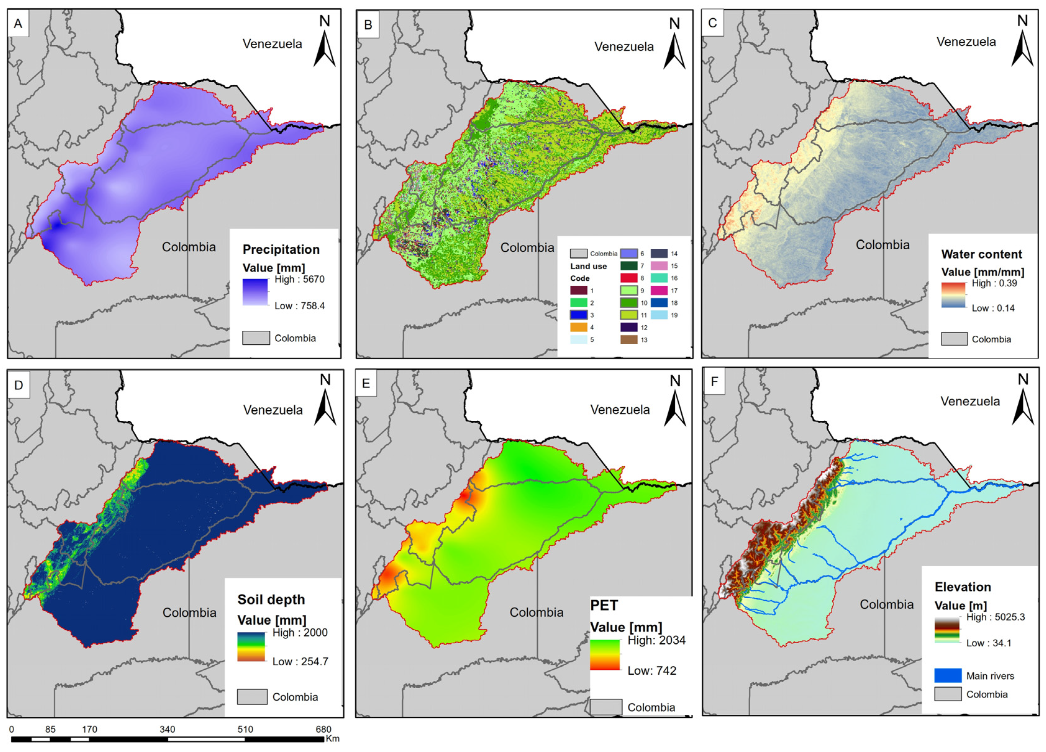
The meteorological data used in this study, including annual precipitation (Figure 2A), annual average water discharge, and annual mean maximum and minimum air temperature, were obtained from the IDEAM (Instituto de Hidrología, Meteorología y Estudios Ambientales) website [58]. We identified 246 hydrometeorological stations measuring air temperature, precipitation, and water discharge in the upper Meta River subbasin, while only one hydrometeorological station measuring water discharge was found in the Yucao River subbasin, and four hydrometeorological stations measuring precipitation and air temperature were in the South Cravo River subbasin. Finally, we found 20 hydrometeorological stations in the upper Casanare River subbasin. The in-situ gauging station records were available from 1983 onwards. The annual potential evapotranspiration (Figure 2E) was calculated using the Hargreaves equation [59] with air temperature data from in-situ stations and extraterrestrial solar radiation data calculated from [60] using the package environment in R [61]. The resulting data were then spatially interpolated into a resolution of 1 km × 1 km. The following Equation (1) was used to calculate potential evapotranspiration—PET (Eto).
E t o = 0.0023 × R a T m a x T m i n 2 + 17.8 + T m a x T m i n 1 / 2
where Tmax and Tmin are maximum and minimum air temperatures (°C); Ra is the terrestrial radiation (MJ m−2 d−1). The PET, calculated in the upper Meta River, Yucao River, South Cravo River, and upper Casanare River subbasins, ranges from a minimum of 789.5 mm/year in the upper Casanare River subbasin to a maximum of 1834.6 mm/year in the upper Meta River subbasin, with a mean value of 1540.7 mm/year in the latter.

2.2.3. Soil Data

The root restricting layer (RRL), as shown in Figure 2D, is the depth of soil where plant roots cannot grow effectively. For this study, a global raster for plant root restricting layer depth was used from [56]. It was found that the upper Meta River, Yucao River, South Cravo River, and upper Casanare River subbasins have different root restricting layer values, ranging from a minimum of 254.7 mm in the upper Meta River subbasin to a maximum of 2000 mm in the Yucao River subbasin, with a mean value of 1815.1 mm in all zones. RRL values can be influenced by factors such as soil compaction, depth to bedrock, and soil structure [62].
Plant available water content (PAWC) is defined as the difference between the fraction of volumetric field capacity and permanent wilting point. In this study, we utilized the global PAWC raster grid from [57]. This dataset provides AWC for seven soil depth intervals (0 to 200 cm depth) and was merged into a single file using the equation recommended by [57]. PAWC values shown in Figure 2C, range from a minimum of 0.1 mm/mm of soil in the upper Casanare River subbasin to a maximum of 0.4 mm/mm of soil in the upper Meta River subbasin, with a mean value of 0.2 mm/mm of soil in all zones.

2.2.4. Land Use/Land Cover Data and Kc

In this study, we used a map elaborated by IDEAM, which employs land use/cover data from the period 2014–2018 [63]. We processed this map into a raster file that combines the 36 land-use/land-cover (LULC) classes into 19 land-use types (Figure 2B, Table 2). We also generated a biophysical table in comma-separated values (CSV) format that contains information related to the LULC map. This table consists of five columns: land-use (LU) code, LULC description, Kc, root depth, and LULC vegetation.
Kc (crop coefficient) values for agricultural land is a dimensionless value used in agriculture to estimate the water needs of crops at different stages of their growth. The FAO (Food and Agriculture Organization of the United Nations) has developed a widely used set of Kc values for various crops, which are based on research carried out in different climatic regions worldwide. The Kc values range from 0 to 1, where 0 represents no water loss, and 1 represents the maximum water loss; these values were extracted from [64]. Land uses different from crops were found in [65] and adapted to our research.

2.2.5. Water Discharge Data

The present study focuses on five hydrometeorological stations (Table 3). The Aceitico gauging station, which is situated in the downstream area of the study basin, represents the final point of the water outflow from the study area. According to the gauge data reported by IDEAM, the maximum annual average water discharge was reported in 2021 with a value of 9288.5 m3/s. On the other hand, the minimum water discharge was reported in 1992 with a value of 3647.6 m3/s. The long-term (for 1983–2021) annual average water discharge was calculated as 5256.8 m3/s. Details of the meteorological stations used in this study are listed in Table 3. To facilitate statistics and to compare water discharges by stations and by the InVEST–AWY model, it was necessary to divide the annual water yield volume (m3) generated by the InVEST–AWY model by the number of seconds in a standard year (3.156 × 10⁷ s).

2.2.6. Zhang Coefficient

The Zhang coefficient (Z) is a parameter that ranges from 1 to 30 and captures the precipitation pattern and hydrogeological characteristics of the basin. This parameter is not enough to be used as a sensitivity and calibration factor [52]. Ref. [66] carried out a study in Australia and found that Z could be estimated as 0.2 N, where N is the number of rainfall events per year. In this study, we calculated the annual average number of rainfall events (N > 1 mm) for the study basin and divided it by 5 to estimate Z. This basin had an annual average of 177 rainy days during the period 1980–2021, and the Z value was assumed to be 30.

2.2.7. The InVEST–AWY Model

The InVEST–AWY model estimates the relative contributions of water from different parts of a landscape, offering insight into how changes in land use/cover patterns affect annual surface water yield and hydropower production [35]. The water yield module in the InVEST–AWY model is built on the annual average precipitation and the Budyko curve [51]. The annual water yield (AWY) for each pixel follows the Equation (2):
A W Y x = 1 A E T x P X × P x ,
where AET(x) is annual evapotranspiration for each pixel x, and P is annual precipitation for each pixel x. For land with vegetation or land use/cover types (LULC), the evapotranspiration fraction of the water balance is A E T x P x ; it is based on the Budyko curve Expression (3) proposed by [67,68]:
A E T x P x = 1 + P E T x P x 1 + A E T x P x w 1 w ,
where PET(x) is the potential evapotranspiration, which is defined as:
P E T ( x ) = K c ( x ) × E T 0 ( x )
where Kc(x) is the yield coefficient per pixel x and E T 0 is the potential evapotranspiration per pixel x. W(x) is a non-physical parameter that characterizes the natural climatic properties of the soil (Equation (5)):
W x = Z × A W C x P x + 1.25
A W C x is the water available to the plant, and Z is the Zhang coefficient, which depends on annual precipitation.
For other land use/cover (LULC) types, such as open water surface, urban areas, and wetlands, actual evaporation (AET) is calculated directly from the reference evaporation E T 0 x and has an upper limit determined by precipitation (Equation (6)):
A E T x = M i n K c l x × E T 0 x × P x ,
where E T 0 x is the reference evapotranspiration; K c ( l x ) is the evaporation factor for each LULC type. The model generates total and average water yields at the subbasin level.

2.3. Methods

2.3.1. Methodology

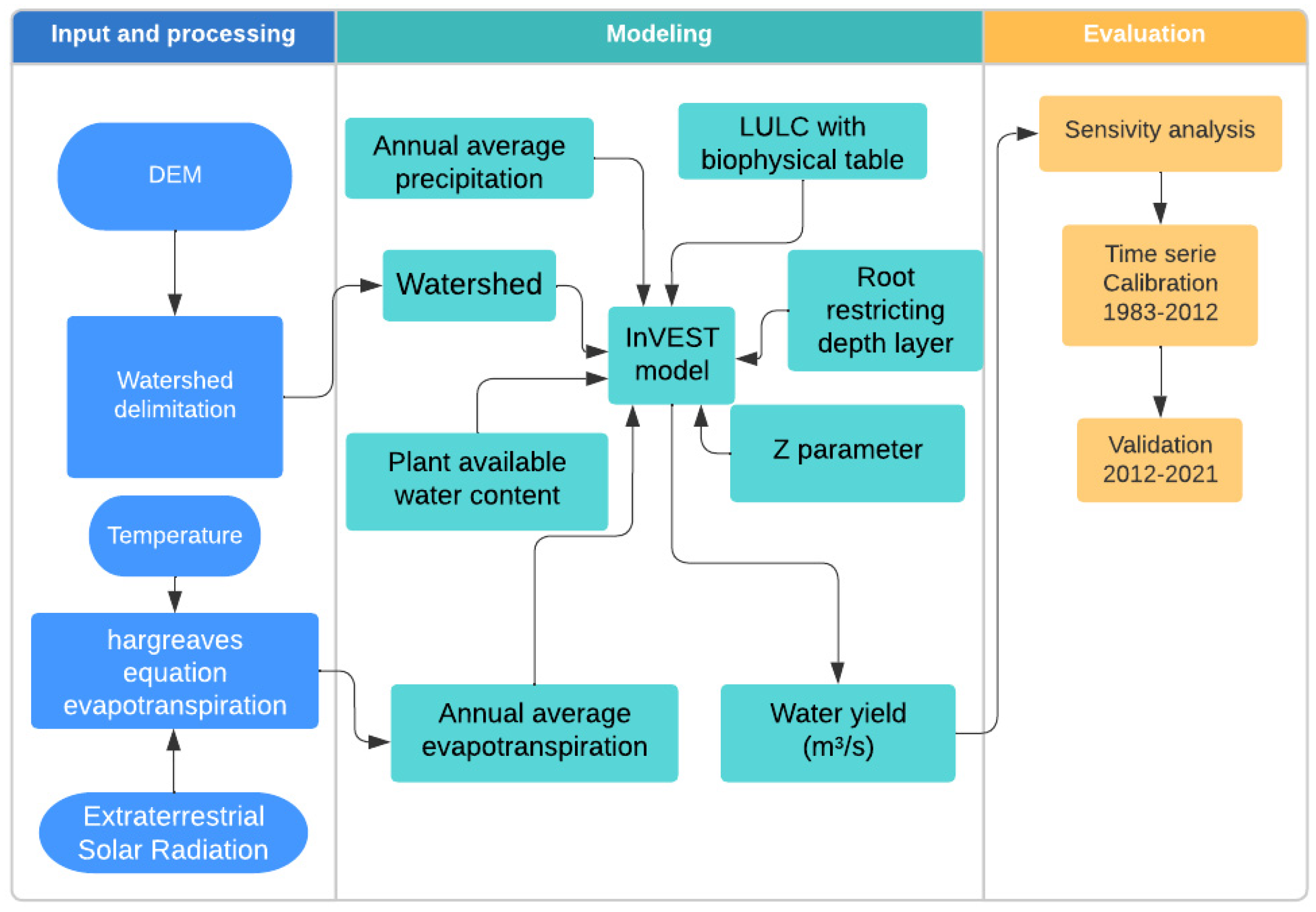
The methodology flowchart adapted from [69] and used in this study is illustrated in Figure 3. The first step of this study involved the preparation of various datasets, including precipitation, reference evapotranspiration, plant available water content, root restricting layer, land use/land cover (LULC) with biophysical table, and watershed delimitation maps. These datasets were essential for accurately modeling water yield in the Meta River basin using the InVEST–AWY model.

2.3.2. Sensitivity Analysis

In the sensitivity analysis, a study carried out by [52] demonstrated that the InVEST–AWY model has low sensitivity with respect to the Zhang coefficient. Nonetheless, this study made in different zones in the UK highlighted the importance of selecting appropriate model parameters and input data, especially precipitation, which had a significant impact on water yield. A 10% increase in precipitation resulted in an 11–27% increase in water yield, while in some catchments, a 10% increase in PET resulted in a 14% decrease in water yield. Rooting depth and AWC had little effect on yield, with a 10% increase in either resulting in a yield decrease of 0–3%. Kc sensitivity was found to be like PET sensitivity. In another study by [19], the model was calibrated for five hydrographic subbasins in Ecuador with Z values ≥ 3 and errors of less than 7%. However, the model could not satisfactorily calibrate the remaining four sub-basins, as water production was underestimated by 20% to 50%. In this study, we carried out a sensitivity analysis for the KC and Zhang coefficients using the 2018 dataset.

Model Sensitivity to Z

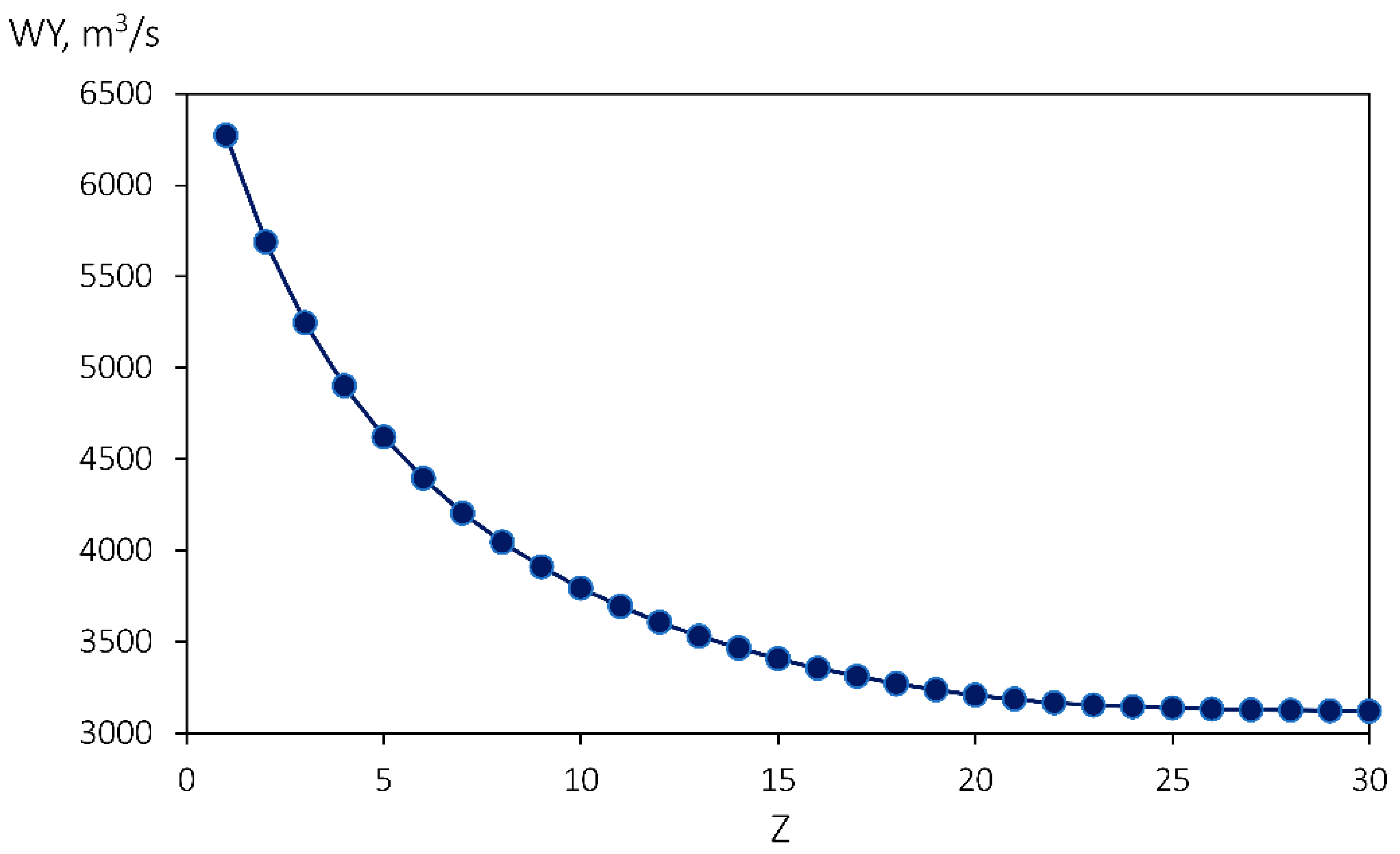
To evaluate the sensitivity of the Zhang coefficient, we used a baseline value of Z = 30, which is defined as the number of rainfall days in a year divided by 5. As stated earlier, the average number of rainfall days for the study zone is 177. As the Z value ranges from 1 to 30, we decreased this value to 1 to evaluate the change in water yield. Our findings indicate that when Z = 15, the water yield increased by 9%, but when Z = 1, the water yield increased by 101% (Figure 4).

Model Sensitivity to Kc

To evaluate the sensitivity of water yield to Kc, we varied this value only for the crop covers in the study zone. The FAO has proposed Kc values for crops found in the Meta River basin that vary between 0.4 and 1.2. We used the baseline Kc values shown in Table 2 and subsequently multiplied them by 0.7, 0.8, 1.2, and 1.3 to evaluate the changes in water yield resulting from the variation in Kc values (Table 4).
The results of the sensitivity analysis showed that a 30% reduction in Kc values in crops would result in a 10.7% decrease in water yield, while increasing Kc values by 30% would only increase water yield by 2%. These findings demonstrate that the Kc value is not a key sensitivity factor for the InVEST–AWY model, unlike Z.

2.3.3. Calibration and Validation

Water yield, the net amount of water produced by a catchment, is a critical factor for sustainable water resource management. It can be estimated by calculating the difference between precipitation and actual evapotranspiration for each LULC type within the catchment [45]. To achieve accurate estimates of water yield, calibration and validation of the model using observed data are essential. A sensitivity analysis is also necessary to determine the variation in the model parameters. Once the optimal parameters have been identified, they can be used for final calibration and validation.
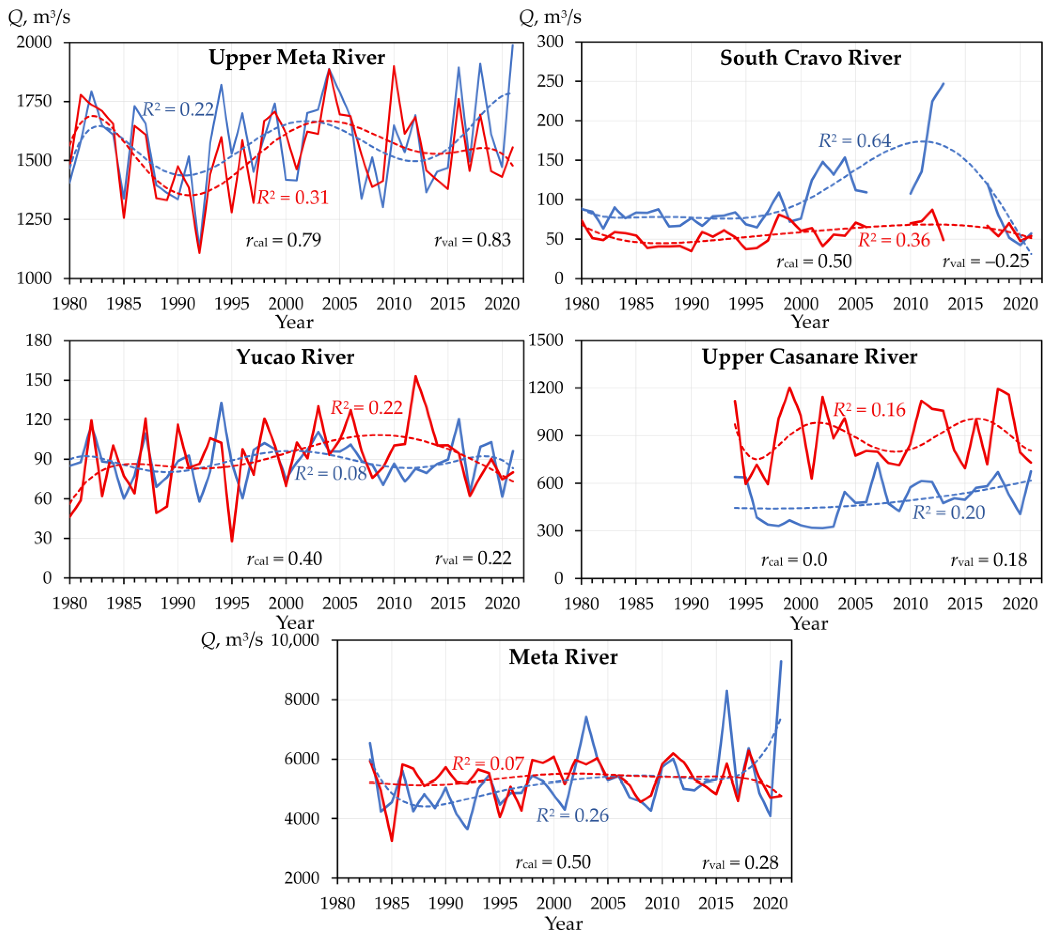
The InVEST–AWY model was calibrated using annual data from 1983 to 2012, which were available at the Aceitico gauging station. The validation period covered the years from 2013 to 2021 (Figure 5). The performance of the model was evaluated by minimizing the average bias and optimizing the coefficient of determination (R2), and Root Mean Square Error (RMSE).
The calibration process involved the use of the InVEST–AWY model in Python. We employed the Automatic Hyperparameter Optimization (AHO) algorithm to identify the best-calibrated model series generated by the InVEST–AWY model using machine learning [70]. We modeled 100 runs for each year from 1983 to 2012, varying the Kc and Z parameters. Based on the interactions, it was found that the InVEST–AWY model performed best when Z = 1 and Kc = 1.10.
However, despite finding the best combination of parameters for the Meta River basin, only the upper Meta River subbasin displayed high correlation coefficients during both calibration (0.79) and validation (0.83) phases, indicating that the model captured the observed data well for this zone. Conversely, the Yucao and South Cravo rivers had lower correlation coefficients, 0.4 and −0.25, respectively, indicating that the model may not be well-suited for these zones, particularly during the validation phase. The upper Casanare River showed no correlation during calibration, but an improvement was noted during validation (0.18), which implies that the model may need further refinement for this zone. The Meta River exhibited moderate correlation coefficients during both calibration (0.5) and validation (0.28), suggesting that the model performed reasonably well, but improvements may be needed. Details for each subbasin are listed in Table 5.
The accurate estimation of water yield is essential for understanding the water balance of a catchment, but the calibration and validation phases may be affected by various factors such as bypassing of gauging stations, catchment transfers, and subsurface runoff [52] found that catchments where a significant proportion of the total water yield leaves via subsurface runoff or other routes were characterized by a significant overestimation of the total yield as gauged from water discharge. In addition, ref. [71] discovered that catchments with a high cover of land-use and land-cover (LULC) classes with a high value of Kc are sensitive to precipitation data, potentially leading to a 150% change in modeled water yield in response to a 30% error.

3. Results, Discussion, and Limitations

3.1. Water Yield Formation

Based on the InVEST–AWY model, we estimated the annual water yield for the Meta River basin from 1983 to 2021. For example, our analysis indicated that the total water yield for the basin in 2018 was 1.98 × 10¹¹ m3/year (6273.4 m3/s or 1748.6 mm/year (Figure 6)), which is 1.3% lower than the value reported by IDEAM. The mean precipitation was found to be 2517.3 mm/year; the mean actual evapotranspiration (AET) was 768.7 mm/year.
In the upper Meta River subbasin, where the model performed better, we obtained a coefficient of determination (R2) of 0.55 and Nash–Sutcliffe Efficiency coefficient (NSE) of 0.49 from 1983 to 2021, using the same parameters as the Meta River basin. The results in the upper Meta River subbasin were found to be directly related to the high density of hydrometeorological stations in the area, as the model is highly sensitive to precipitation and evapotranspiration [44,48].
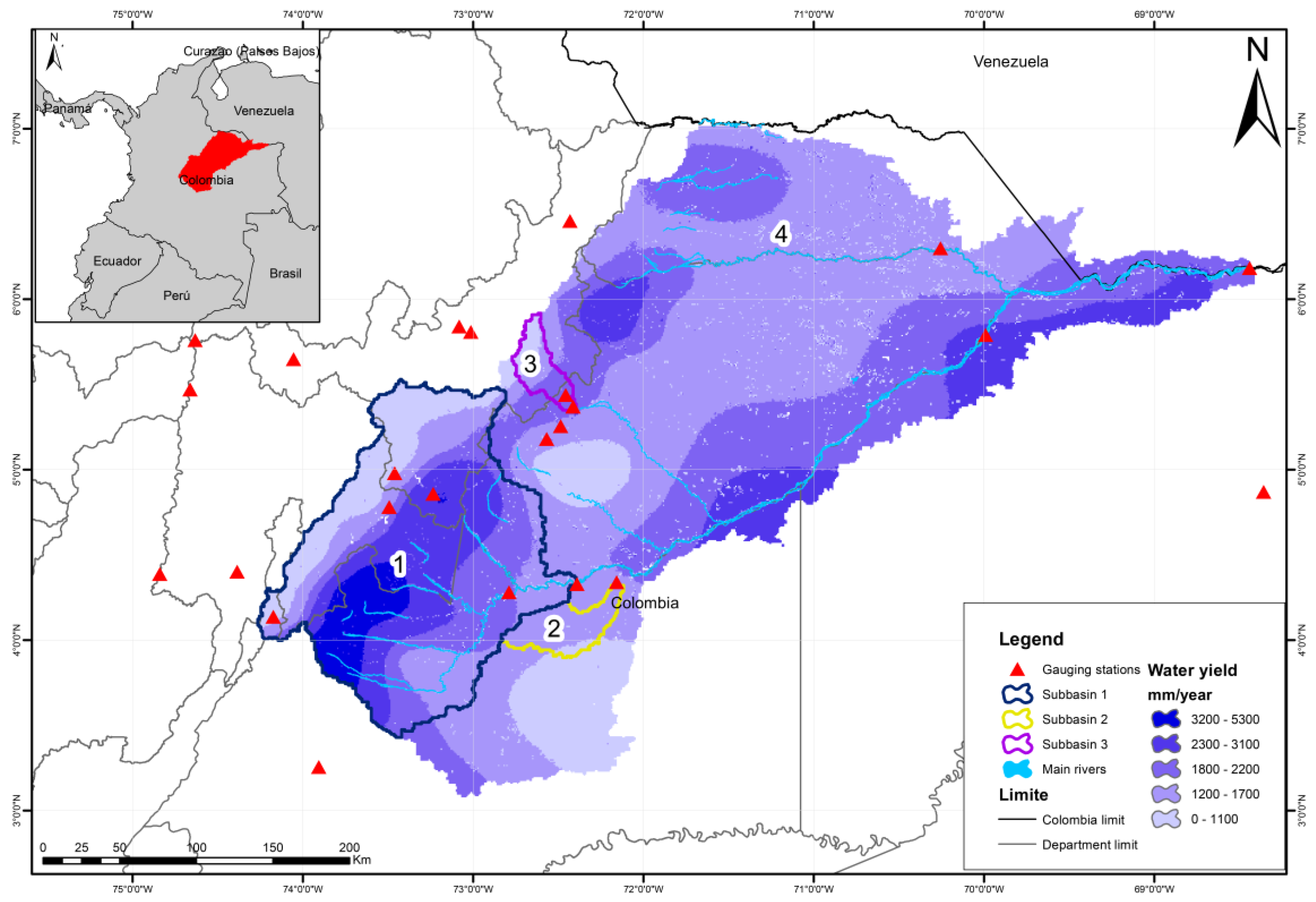
The spatial patterns analysis revealed that the annual water yield exhibited higher values in the northwest of the basin, particularly in the first delimited subbasin, with variations ranging from 1100 to 5300 mm/year. On the other hand, other annual water yield values showed a significant pattern in the southeast of the basin, which represents the lowest part of the study area and where the rivers merge to form the Meta River.
To assess the effectiveness of the model, statistics were computed for five studied zones where the InVEST–AWY model tool was applied. The full climatological dataset from 1983 to 2021 was utilized to evaluate various performance metrics, including Nash–Sutcliffe Efficiency (NSE) coefficient, Root Mean Square Error (RMSE), R-squared (R2), and standard deviation of the differences (DIF STD) between observed and modeled data. The results of the evaluation are presented in Table 5, which provides a detailed breakdown of the model’s performance in each studied zone.
The results of hydrological modeling showed that the Meta River basin had poor performance, with an NSE value of 0.07 and a high RMSE value of 1071.61. The correlation coefficients during calibration (rcal) and validation (rval) were low (0.50 and 0.28, respectively), indicating that the model had low accuracy in predicting the observed annual water discharge. The complexity of the basin’s climate and topography, as well as a deficient hydrometeorological monitoring system, could be contributing factors to these results.
The upper Meta River subbasin had the best performance among all subbasins, with an NSE value of 0.49 and a low RMSE value of 135.37. The correlation coefficient values for calibration and validation periods were high (0.79 and 0.83, respectively), indicating that the model had high accuracy in predicting the observed annual water discharge. This could be since the upper Meta River subbasin is the area with the greatest presence of hydrometeorological stations that allows accurate monitoring.
The Yucao River subbasin had moderate performance, with an NSE value of 0.03 and a moderate RMSE value of 57.49. The correlation coefficient during calibration was high (0.40), suggesting that the model had a good ability to capture the variability of the observed annual water discharge. However, the coefficient of determination during validation was low (0.22), indicating that the model had low accuracy in predicting the observed annual water discharge.
The South Cravo River subbasin had the worst performance among all subbasins, with an NSE value of −1.29 and a low RMSE value of 24.75. The correlation coefficients for calibration and validation (rcal and rval) periods were also low (0.50 and −0.25, respectively), indicating that the model had low accuracy in predicting the observed annual water discharge.
The upper Casanare River subbasin had very poor performance, with a negative NSE value of −0.49 and a high RMSE value of 452.32. The correlation coefficients were low for calibration and validation periods (0 and 0.18, respectively), suggesting that the model had low accuracy in predicting the observed annual water discharge. The upper Casanare River subbasin has a heterogeneous land use pattern and complex surface and underground hydraulic dynamics, which could have made it challenging to model the hydrological processes accurately.

3.2. Limitations

3.2.1. Model Limitations

The model relies on yearly averages and disregards temporal (including seasonal) variations in water supply and hydropower production, leading to inadequate estimations of water availability and energy production during extreme events such as droughts or floods. In addition, the model oversimplifies the concept of consumptive demand, which can impact its precision in estimating water availability for various purposes. Consequently, this constraint can have substantial implications in evaluating the effects of LULC changes on water resources [35].
The InVEST–AWY model simplifies the hydrological process by lacking differentiation between surface and subsurface water runoff. Consequently, this oversimplification introduces several uncertainties in the model simulation [50].
The model exhibits low sensitivity to modifications in the Z coefficient, but it is highly sensitive to precipitation. Therefore, it is imperative to evaluate the precision of yearly data [48].

3.2.2. Uncertainties from In-Situ Data

The lack of hydrogeological studies in the Meta River basin poses a limitation in identifying the hydrogeological dynamics that may influence the percentage of groundwater contribution to the primary rivers measured by IDEAM stations. Nonetheless, a study carried out by [9] revealed the existence of groundwater wells with hydraulic transmissivity ranging between 4 to 279 m2/day in the northeastern region of the study basin, which could mean a varied water dynamics in aquifers.
The study is subject to uncertainties of the model due to the insufficiency of information from the selected stations. One of the five stations used for the study is automated. Moreover, data gaps were observed for several stations within the study area, including the Aceitico gauging station, which lacks annual data from 1980 to 1982 and reported atypical values in 2003, 2016, and 2021. Similarly, for the Cravo Norte gauging station, there was a gap in information from 1980 to 1993; in Puente Yopal, there were also gaps in annual water discharge data for 2007–2009 and 2014–2016. These gaps in information and atypical values could affect the accuracy of the model’s calibration and validation, thus limiting its ability to provide precise estimations of water runoff in the study area.

3.2.3. Human Effect on Water Discharge

According to [72], the change in water runoff in the Meta River basin cannot be solely attributed to macroclimatic phenomena or human activities on the local scale. Meanwhile, [18] reported that groundwater extraction provides about 5% of the total demand from various sectors in the region, but the actual value could be higher due to unreported or illegal extractions.

4. Conclusions

While the InVEST–AWY model did not show satisfied results for the Meta River basin as a whole, our study demonstrated that the model could be a valuable tool for identifying subbasins where it could work adequately. This allows for the establishment of selection criteria for areas of interest.
In our study, we identified the upper Meta River subbasin delimited for the Humapo gauging station as having the most climate monitoring stations in the study area. However, due to a lack of hydrogeological studies in the area, it is difficult to establish the proven uncertainty of groundwater contribution to surface runoff measured by IDEAM stations.
Atypical events, such as those reported during 2003, 2016, and 2021, have been observed at the stations that are not related to El Niño and La Niña fluctuations. These reports should be analyzed on a daily scale and related to multiple climatic and anthropogenic variables to better understand their causes.
In future studies, it is important to consider using the InVEST “Annual Water Yield” model in areas with a high density of weather stations. Alternatively, global data such as CHIRPS can be used, with necessary corrections for overestimation or underestimation of precipitation. It is also crucial to validate the calculated evapotranspiration with in-situ data reported by the authorities.

Author Contributions

Conceptualization, J.B.V. and V.V.G.; methodology, J.B.V., V.V.G. and J.M.-D.; analysis, J.B.V. and J.M.-D.; data curation, J.B.V. and J.M.-D.; writing—original draft preparation, J.B.V.; writing—review and editing, J.B.V., A.V.G. and J.T.; visualization, J.B.V., A.V.G. and J.M.-D.; supervision, J.B.V. and J.T. All authors have read and agreed to the published version of the manuscript.

Funding

The work was carried out in accordance with the Strategic Academic Leadership Program “Priority 2030” of the Kazan Federal University of the Government of the Russian Federation.

Data Availability Statement

Data used for this research can be obtained upon request from the authors.

Acknowledgments

We would like to thank Nilton Díaz from the Alliance Bioversity International—CIAT for technical advice on the evaluation of the InVEST–AWY model for annual water discharges in the subbasins of the Meta River basin. We would also like to thank IDEAM for providing timely climate data for the study area.

Conflicts of Interest

The authors declare no conflict of interest.

References

  1. Belhassan, K. Water Scarcity Management. In Water Safety, Security and Sustainability: Threat Detection and Mitigation; Vaseashta, A., Maftei, C., Eds.; Advanced Sciences and Technologies for Security Applications; Springer International Publishing: Cham, Switzerland, 2021; pp. 443–462. ISBN 978-3-030-76008-3. [Google Scholar]
  2. Boretti, A.; Rosa, L. Reassessing the Projections of the World Water Development Report. Npj Clean Water 2019, 2, 15. [Google Scholar] [CrossRef]
  3. Cosgrove, W.; Loucks, P. Water Management: Current and Future Challenges and Research Directions. Water Resour. Res. 2015, 51, 4823–4839. [Google Scholar] [CrossRef]
  4. Milly, P.C.D.; Dunne, K.A.; Vecchia, A.V. Global Pattern of Trends in Streamflow and Water Availability in a Changing Climate. Nature 2005, 438, 347–350. [Google Scholar] [CrossRef] [PubMed]
  5. Célleri, R.; Feyen, J. The Hydrology of Tropical Andean Ecosystems: Importance, Knowledge Status, and Perspectives. Mt. Res. Dev. 2009, 29, 350–355. [Google Scholar] [CrossRef]
  6. Acuña, G.J.; Ávila, H.; Canales, F.A. River Model Calibration Based on Design of Experiments Theory. A Case Study: Meta River, Colombia. Water 2019, 11, 1382. [Google Scholar] [CrossRef]
  7. Ávila, H.; Acuña, G.; Daza, R.; Diaz, K.S. Evaluating the Natural Development of the Meta River for Proposing Hydraulic Works Oriented to River Training for Fluvial Navigation. In Proceedings of the World Environmental and Water Resources Congress 2014, Portland, OR, USA, 1–5 June 2014; pp. 1564–1579. [Google Scholar] [CrossRef]
  8. DNP: BASES DEL PLAN NACIONAL DE DESARROLLO 2018–2022. 2018. Available online: https://colaboracion.dnp.gov.co/CDT/Prensa/BasesPND2018-2022n.pdf (accessed on 18 February 2023).
  9. Benavides Guerrero, C.E.; Caro Caro, L.E.; Mariño Martínez, J.E. Determination of the Hydraulic Behavior of Aquifers in Northern Orinoquia, Colombia. Cienc. E Ing. Neogranadina 2021, 31, 109–126. [Google Scholar] [CrossRef]
  10. Garcia, N. Evaluation of Rainfall Runnoff Modelling Using BROOK90 in R in a Case Study of a Catchment Area in Colombia. Master’s Thesis, Dresden University of Technology, Dresden, Germany, 2019. [Google Scholar]
  11. Hoyos, N.; Correa-Metrio, A.; Jepsen, S.M.; Wemple, B.; Valencia, S.; Marsik, M.; Doria, R.; Escobar, J.; Restrepo, J.C.; Velez, M.I. Modeling Streamflow Response to Persistent Drought in a Coastal Tropical Mountainous Watershed, Sierra Nevada De Santa Marta, Colombia. Water 2019, 11, 94. [Google Scholar] [CrossRef]
  12. Moncada, A.M.; Escobar, M.; Betancourth, A.; Vélez Upegui, J.J.; Zambrano, J.; Alzate, L.M. Modelling Water Stress Vulnerability in Small Andean Basins: Case Study of Campoalegre River Basin, Colombia. Int. J. Water Resour. Dev. 2021, 37, 640–657. [Google Scholar] [CrossRef]
  13. Person, M.; Butler, D.; Gable, C.; Villamil, T.; Wavrek, D.; Schelling, D. Hydrodynamic Stagnation Zones: A New Play Concept for the Llanos Basin, Colombia. AAPG Bull. 2012, 96, 23–41. [Google Scholar] [CrossRef]
  14. Ramirez Morales, W.D.; Rodriguez, E.A.; Sanchez Lozano, J.L.; Oliveros-Acosta, J.J.; Ardila, F.; Cardona-Almeida, C.; Garay, C.; Bouaziz, L. Hydrologic Modeling of Principal Sub-Basins of the Magdalena-Cauca Large Basin Using Wflow Model. In Proceedings of the 36th International Association for Hydro-Environment Engineering and Research World Congress, The Hague, The Netherlands, 2 July 2015. [Google Scholar]
  15. Restrepo, J.D.; Kjerfve, B.; Hermelin, M.; Restrepo, J.C. Factors Controlling Sediment Yield in a Major South American Drainage Basin: The Magdalena River, Colombia. J. Hydrol. 2006, 316, 213–232. [Google Scholar] [CrossRef]
  16. Rodríguez, E.; Sánchez, I.; Duque, N.; Arboleda, P.; Vega, C.; Zamora, D.; López, P.; Kaune, A.; Werner, M.; García, C.; et al. Combined Use of Local and Global Hydro Meteorological Data with Hydrological Models for Water Resources Management in the Magdalena—Cauca Macro Basin—Colombia. Water Resour. Manag. 2020, 34, 2179–2199. [Google Scholar] [CrossRef]
  17. Villamizar, S.R.; Pineda, S.M.; Carrillo, G.A. The Effects of Land Use and Climate Change on the Water Yield of a Watershed in Colombia. Water 2019, 11, 285. [Google Scholar] [CrossRef]
  18. Pimentel, J.N.; Rogéliz Prada, C.A.; Walschburger, T. Hydrological Modeling for Multifunctional Landscape Planning in the Orinoquia Region of Colombia. Front. Environ. Sci. 2021, 9, 673215. [Google Scholar] [CrossRef]
  19. Minga-León, S.; Gómez-Albores, M.A.; Bâ, K.M.; Balcázar, L.; Manzano-Solís, L.R.; Cuervo-Robayo, A.P.; Mastachi-Loza, C.A. Estimation of Water Yield in the Hydrographic Basins of Southern Ecuador. Hydrol. Earth Syst. Sci. Discuss. 2018, 1–18. [Google Scholar] [CrossRef]
  20. Kumari, N.; Srivastava, A.; Sahoo, B.; Raghuwanshi, N.S.; Bretreger, D. Identification of Suitable Hydrological Models for Streamflow Assessment in the Kangsabati River Basin, India, by Using Different Model Selection Scores. Nat. Resour. Res. 2021, 30, 4187–4205. [Google Scholar] [CrossRef]
  21. Shekar, P.R. Rainfall-Runoff Modelling of a River Basin Using HEC HMS: A Review Study. Int. J. Res. Appl. Sci. Eng. Technol. 2021, 9, 506–508. [Google Scholar] [CrossRef]
  22. Gashaw, T.; Worqlul, A.W.; Dile, Y.T.; Sahle, M.; Adem, A.A.; Bantider, A.; Teixeira, Z.; Alamirew, T.; Meshesha, D.T.; Bayable, G. Evaluating InVEST Model for Simulating Annual and Seasonal Water Yield in Data-Scarce Regions of the Abbay (Upper Blue Nile) Basin: Implications for Water Resource Planners and Managers. Sustain. Water Resour. Manag. 2022, 8, 170. [Google Scholar] [CrossRef]
  23. Zaccaria, D.; Neale, C.M.U.; Lamaddalena, N. A Methodology for Conducting Diagnostic Analyses and Operational Simulation in Large-Scale Pressurized Irrigation Systems. SPIE Proc. 2006, 63, 5910. [Google Scholar] [CrossRef]
  24. Chen, Y.; Li, J.; Huang, S.; Dong, Y. Study of Beijiang Catchment Flash-Flood Forecasting Model. Proc. Int. Assoc. Hydrol. Sci. 2015, 368, 150–155. [Google Scholar] [CrossRef]
  25. Belay, Y.Y.; Gouday, Y.A.; Alemnew, H.N. Comparison of HEC-HMS Hydrologic Model for Estimation of Runoff Computation Techniques as a Design Input: Case of Middle Awash Multi-Purpose Dam, Ethiopia. Appl. Water Sci. 2022, 12, 237. [Google Scholar] [CrossRef]
  26. Yen, H.; Jeong, J.; Feng, Q.; Deb, D. Assessment of Input Uncertainty in SWAT Using Latent Variables. Water Resour. Manag. 2015, 29, 1137–1153. [Google Scholar] [CrossRef]
  27. Brulebois, E.; Ubertosi, M.; Castel, T.; Richard, Y.; Sauvage, S.; Sánchez Pérez, J.; Moine, N.; Suchet, P. Robustness and Performance of Semi-Distributed (SWAT) and Global (GR4J) Hydrological Models throughout an Observed Climatic Shift over Contrasted French Watersheds. Open Water J. 2018, 5, 4. [Google Scholar]
  28. Haris, A.A.; Khan, M.A.; Chhabra, V.; Biswas, S.; Pratap, A. Evaluation of LARS-WG for Generating Long Term Data for Assessment of Climate Change Impact in Bihar. J. Agrometeorol. 2010, 12, 198–201. [Google Scholar] [CrossRef]
  29. Fu, B.; Merritt, W.S.; Croke, B.F.W.; Weber, T.R.; Jakeman, A.J. A Review of Catchment-Scale Water Quality and Erosion Models and a Synthesis of Future Prospects. Environ. Model. Softw. 2019, 114, 75–97. [Google Scholar] [CrossRef]
  30. Pandi, D.; Kothandaraman, S.; Kuppusamy, M. Hydrological Models: A Review. Int. J. Hydrol. Sci. Technol. 2021, 12, 223–242. [Google Scholar] [CrossRef]
  31. Decsi, B.; Ács, T.; Jolánkai, Z.; Kardos, M.K.; Koncsos, L.; Vári, Á.; Kozma, Z. From Simple to Complex—Comparing Four Modelling Tools for Quantifying Hydrologic Ecosystem Services. Ecol. Indic. 2022, 141, 109143. [Google Scholar] [CrossRef]
  32. Scordo, F.; Lavender, T.M.; Seitz, C.; Perillo, V.L.; Rusak, J.A.; Piccolo, M.C.; Perillo, G.M.E. Modeling Water Yield: Assessing the Role of Site and Region-Specific Attributes in Determining Model Performance of the InVEST Seasonal Water Yield Model. Water 2018, 10, 1496. [Google Scholar] [CrossRef]
  33. Posner, S.; Verutes, G.; Koh, I.; Denu, D.; Ricketts, T. Global Use of Ecosystem Service Models. Ecosyst. Serv. 2016, 17, 131–141. [Google Scholar] [CrossRef]
  34. Shrestha, D.L. Uncertainty Analysis in Rainfall-Runoff Modelling—Application of Machine Learning Techniques: UNESCO-IHE PhD Thesis; Taylor & Francis: Abingdon, UK, 2009. [Google Scholar]
  35. Natural Capital Project Seasonal Water Yield—InVEST 3.6.0 Documentation. Available online: http://data.naturalcapitalproject.org/nightly-build/invest-users-guide/html/seasonal_water_yield.html (accessed on 4 May 2020).
  36. Wei, Y.-M.; Kang, J.-N.; Liu, L.-C.; Li, Q.; Wang, P.-T.; Hou, J.-J.; Liang, Q.-M.; Liao, H.; Huang, S.-F.; Yu, B. A Proposed Global Layout of Carbon Capture and Storage in Line with a 2 °C Climate Target. Nat. Clim. Chang. 2021, 11, 112–118. [Google Scholar] [CrossRef]
  37. Florian-Vergara, C.; Salas, H.D.; Builes-Jaramillo, A. Analysis of Precipitation and Evaporation in the Colombian Orinoco According to the Regional Climate Models of the CORDEX-CORE Experiment. TecnoLógicas 2021, 24, 242–261. [Google Scholar] [CrossRef]
  38. Vásquez, E. The Orinoco River: A Review of Hydrobiological Research. Regul. Rivers Res. Manag. 1989, 3, 381–392. [Google Scholar] [CrossRef]
  39. Gimeno, L.; Gallego, D.; Trigo, R.M.; Ribera, P. Dynamic Identification of Moisture Sources in the Orinoco Basin in Equatorial South America. Hydrol. Sci. J. 2008, 53, 602–617. [Google Scholar] [CrossRef]
  40. Essou, G.R.C.; Brissette, F.; Lucas-Picher, P. The Use of Reanalyses and Gridded Observations as Weather Input Data for a Hydrological Model: Comparison of Performances of Simulated River Flows Based on the Density of Weather Stations. J. Hydrometeorol. 2017, 18, 497–513. [Google Scholar] [CrossRef]
  41. Rajib, A.; Merwade, V.; Yu, Z. Rationale and Efficacy of Assimilating Remotely Sensed Potential Evapotranspiration for Reduced Uncertainty of Hydrologic Models. Water Resour. Res. 2018, 54, 4615–4637. [Google Scholar] [CrossRef]
  42. Krishnan, R. Bayesian Parameter Uncertainty Modeling in a Macroscale Hydrologic Model and Its Impact on Indian River Basin Hydrology under Climate Change. Water Resour. Res. 2012, 48, 8522. [Google Scholar] [CrossRef]
  43. Trudel, M.; Doucet-Généreux, P.-L.; Leconte, R. Assessing River Low-Flow Uncertainties Related to Hydrological Model Calibration and Structure under Climate Change Conditions. Climate 2017, 5, 19. [Google Scholar] [CrossRef]
  44. Hamel, P.; Guswa, A.J. Uncertainty Analysis of a Spatially Explicit Annual Water-Balance Model: Case Study of the Cape Fear Basin, North Carolina. Hydrol. Earth Syst. Sci. 2015, 19, 839–853. [Google Scholar] [CrossRef]
  45. Li, M.; Liang, D.; Xia, J.; Song, J.; Cheng, D.; Wu, J.; Cao, Y.; Sun, H.; Li, Q. Evaluation of Water Conservation Function of Danjiang River Basin in Qinling Mountains, China Based on InVEST Model. J. Environ. Manag. 2021, 286, 112212. [Google Scholar] [CrossRef]
  46. Li, Z.; Deng, X.; Jin, G.; Mohmmed, A.; Arowolo, A.O. Tradeoffs between Agricultural Production and Ecosystem Services: A Case Study in Zhangye, Northwest China. Sci. Total Environ. 2020, 707, 136032. [Google Scholar] [CrossRef]
  47. Wang, X.; Liu, G.; Lin, D.; Lin, Y.; Lu, Y.; Xiang, A.; Xiao, S. Water Yield Service Influence by Climate and Land Use Change Based on InVEST Model in the Monsoon Hilly Watershed in South China. Geomat. Nat. Hazards Risk 2022, 13, 2024–2048. [Google Scholar] [CrossRef]
  48. Yang, D.; Liu, W.; Tang, L.; Chen, L.; Li, X.; Xu, X. Estimation of Water Provision Service for Monsoon Catchments of South China: Applicability of the InVEST Model. Landsc. Urban Plan. 2019, 182, 133–143. [Google Scholar] [CrossRef]
  49. Yin, G.; Wang, X.; Zhang, X.; Fu, Y.; Hao, F.; Hu, Q. InVEST Model-Based Estimation of Water Yield in North China and Its Sensitivities to Climate Variables. Water 2020, 12, 1692. [Google Scholar] [CrossRef]
  50. Yu, Y.; Sun, X.; Wang, J.; Zhang, J. Using InVEST to Evaluate Water Yield Services in Shangri-La, Northwestern Yunnan, China. PeerJ 2022, 10, e12804. [Google Scholar] [CrossRef]
  51. Budyko, M.I. Climate and Life; Academic Press: Cambridge, MA, USA, 1974. [Google Scholar]
  52. Redhead, J.W.; Stratford, C.; Sharps, K.; Jones, L.; Ziv, G.; Clarke, D.; Oliver, T.H.; Bullock, J.M. Empirical Validation of the InVEST Water Yield Ecosystem Service Model at a National Scale. Sci. Total Environ. 2016, 569–570, 1418–1426. [Google Scholar] [CrossRef] [PubMed]
  53. Almeida, B.; Cabral, P. Water Yield Modelling, Sensitivity Analysis and Validation: A Study for Portugal. ISPRS Int. J. Geo-Inf. 2021, 10, 494. [Google Scholar] [CrossRef]
  54. Dennedy-Frank, P.J.; Muenich, R.L.; Chaubey, I.; Ziv, G. Comparing Two Tools for Ecosystem Service Assessments Regarding Water Resources Decisions. J. Environ. Manag. 2016, 177, 331–340. [Google Scholar] [CrossRef] [PubMed]
  55. Chacko, S.; Kurian, J.S.; Ravichandran, C.; Vairavel, S.M.; Kumar, K. An Assessment of Water Yield Ecosystem Services in Periyar Tiger Reserve, Southern Western Ghats of India. Geol. Ecol. Landsc. 2019, 5, 32–39. [Google Scholar] [CrossRef]
  56. Yang, Y.; Donohue, R.J.; McVicar, T.R. Global Estimation of Effective Plant Rooting Depth: Implications for Hydrological Modeling. Water Resour. Res. 2016, 52, 8260–8276. [Google Scholar] [CrossRef]
  57. Hengl, T.; de Jesus, J.M.; Heuvelink, G.B.M.; Gonzalez, M.R.; Kilibarda, M.; Blagotić, A.; Shangguan, W.; Wright, M.N.; Geng, X.; Bauer-Marschallinger, B.; et al. SoilGrids250m: Global Gridded Soil Information Based on Machine Learning. PLoS ONE 2017, 12, e0169748. [Google Scholar] [CrossRef]
  58. IDEAM Consulta y Descarga de Datos Hidrometeorológicos. Available online: http://dhime.ideam.gov.co/atencionciudadano/ (accessed on 19 February 2023).
  59. Hargreaves, G.H.; Samani, Z.A. Estimating Potential Evapotranspiration. J. Irrig. Drain. Div. 1982, 108, 225–230. [Google Scholar] [CrossRef]
  60. Laskar, J.; Robutel, P.; Joutel, F.; Gastineau, M.; Correia, A.C.M.; Levrard, B. A Long-Term Numerical Solution for the Insolation Quantities of the Earth. Astron. Astrophys. 2004, 428, 261–285. [Google Scholar] [CrossRef]
  61. R: Extraterrestrial Solar Radiation. Available online: https://search.r-project.org/CRAN/refmans/envirem/html/ETsolradRasters.html (accessed on 19 February 2023).
  62. Peth, S. Soil Compactibility and Compressibility. In Encyclopedia of Agrophysics; Gliński, J., Horabik, J., Lipiec, J., Eds.; Encyclopedia of Earth Sciences Series; Springer: Dordrecht, The Netherlands, 2011; pp. 742–745. ISBN 978-90-481-3585-1. [Google Scholar]
  63. IDEAM Mapas de Suelos del Territorio Colombiano a Escala 1:100.000. 2018. Available online: http://www.siac.gov.co/catalogo-de-mapas (accessed on 19 February 2023).
  64. Allen, R.; Pereira, L.; Raes, D.; Smith, M. Evapotranspiración del Cultivo: Guias para la Determinación de los Requerimientos de Agua de los Cultivos; FAO: Rome, Italy, 2006. [Google Scholar]
  65. IDEAM METODOLOGÍA PARA LA ZONIFICACIÓN DE SUSCEPTIBILIDAD GENERAL DEL TERRENO A LOS MOVIMIENTOS EN MASA. 2012. Available online: https://bit.ly/3mN5DpE (accessed on 19 February 2023).
  66. Donohue, R.J.; Roderick, M.L.; McVicar, T.R. Roots, Storms and Soil Pores: Incorporating Key Ecohydrological Processes into Budyko’s Hydrological Model. J. Hydrol. 2012, 436–437, 35–50. [Google Scholar] [CrossRef]
  67. Fu, B.P. On the calculation of the evaporation from land surface. Chin. J. Atmos. Sci. 1981, 5, 23–31. [Google Scholar] [CrossRef]
  68. Zhang, Y.; Kendy, E.; Qiang, Y.; Changming, L.; Yanjun, S.; Hongyong, S. Effect of Soil Water Deficit on Evapotranspiration, Crop Yield, and Water Use Efficiency in the North China Plain. Agric. Water Manag. 2004, 64, 107–122. [Google Scholar] [CrossRef]
  69. Bejagam, V.; Keesara, V.R.; Sridhar, V. Impacts of Climate Change on Water Provisional Services in Tungabhadra Basin Using InVEST Model. River Res. Appl. 2022, 38, 94–106. [Google Scholar] [CrossRef]
  70. Bergstra, J.; Yamins, D.; Cox, D.D. Making a Science of Model Search: Hyperparameter Optimization in Hundreds of Dimensions for Vision Architectures. arXiv 2013, arXiv:1209.5111. Available online: https://arxiv.org/abs/1209.5111 (accessed on 17 February 2023).
  71. Pessacg, N.; Flaherty, S.; Brandizi, L.; Solman, S.; Pascual, M. Getting Water Right: A Case Study in Water Yield Modelling Based on Precipitation Data. Sci. Total Environ. 2015, 537, 225–234. [Google Scholar] [CrossRef]
  72. Arrieta-Castro, M.; Donado-Rodríguez, A.; Acuña, G.J.; Canales, F.A.; Teegavarapu, R.S.V.; Kaźmierczak, B. Analysis of Streamflow Variability and Trends in the Meta River, Colombia. Water 2020, 12, 1451. [Google Scholar] [CrossRef]
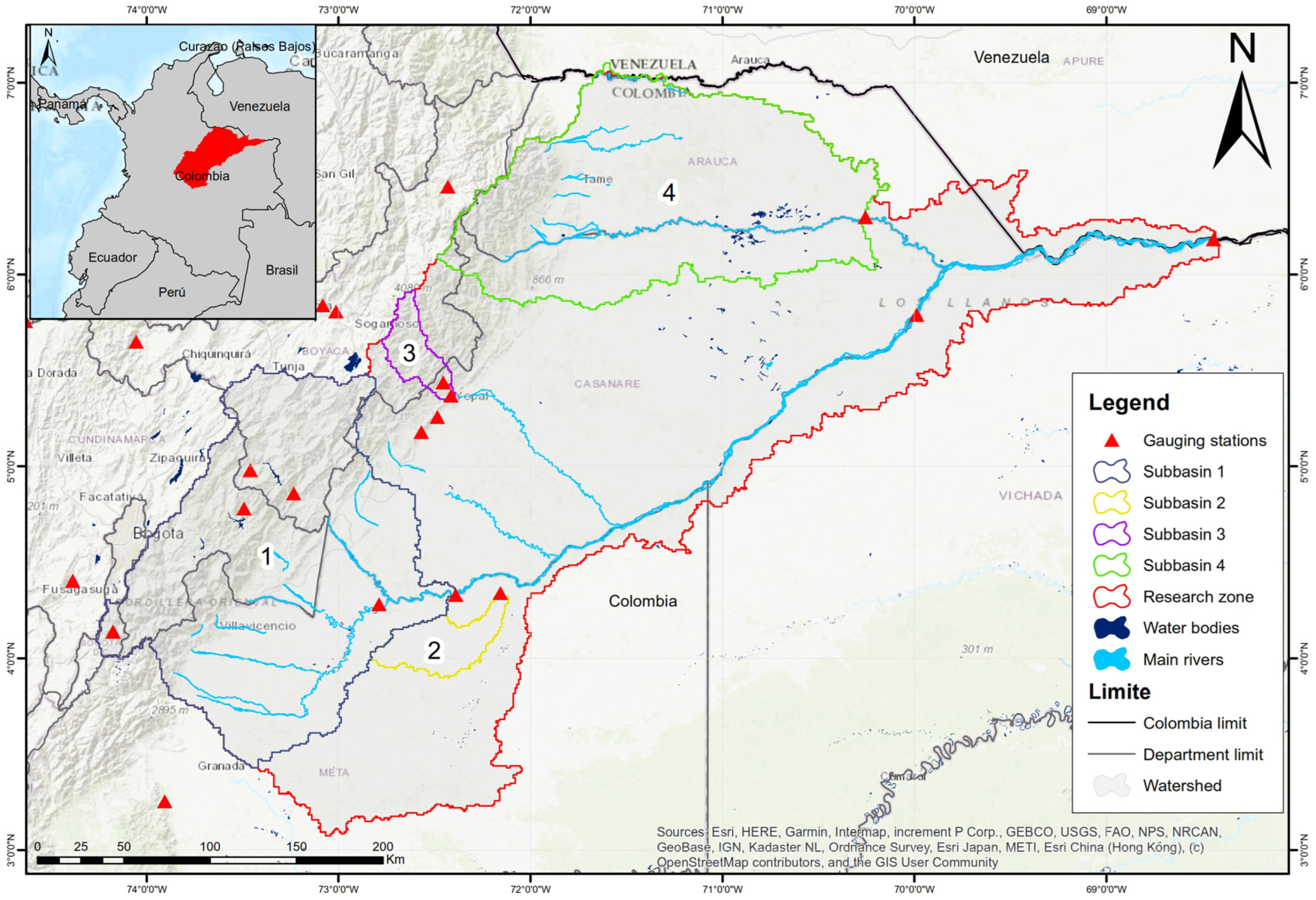
Figure 1. Location of the Meta River basin (Research zone) and its subbasins in Colombia. Subbasin 1: upper Meta River subbasin; Subbasin 2: Yucao River subbasin; Subbasin 3: South Cravo River subbasin; Subbasin 4: upper Casanare River subbasin.
Water 15 01617 g001
Figure 2. Geospatial data for the InVEST–AWY model: (A) Annual precipitation; (B) Different LULC types: 1—urban area, 2–8—crops, 9—pastures, 10—forests, 11–13—shrubby area, 14—sands, 15—rocks, 16—bare grounds, 17—snow cover, 18—aquatic vegetation, and 19—water bodies; (C) Water content in the soil; (D) Soil depth; (E) Potential evapotranspiration (PET); (F) Digital elevation model (DEM).
Water 15 01617 g002
Figure 3. Methodology flowchart for calculation of water yield in the Meta River basin using the InVEST–AWY model.
Water 15 01617 g003
Figure 4. Water yield (WY) variation using different Zhang coefficient (Z).
Water 15 01617 g004
Figure 5. Changes in the observed (solid blue line) and modeled (solid red line) water discharge (Q) of the studied rivers of the Meta River basin for 1980–2021. The dotted line is the sixth-degree polynomial trend of the corresponding (observed or modeled) water discharge. R2 is the coefficient of approximation of the trend line; rcal and rval are the correlation coefficients for the period of calibration (1983–2012) and validation (2013–2021), respectively.
Water 15 01617 g005
Figure 6. Annual water yield formation in the subbasins of the Meta River basin for 2018. (1) upper Meta River subbasin; (2) Yucao River subbasin; (3) South Cravo River subbasin; (4) upper Casanare River subbasin.
Water 15 01617 g006
Table 1. Dataset used in the InVEST–AWY modeling.
DataPeriodSourceToolFormat
Annual average precipitation1983–2021Instituto de Hidrología, Meteorología y Estudios Ambientales—IDEAMRStudioRaster
Annual average water discharge1983–2021Instituto de Hidrología, Meteorología y Estudios Ambientales—IDEAM-CSV
Evapotranspiration1983–2021Instituto de Hidrología, Meteorología y Estudios Ambientales IDEAM (air temperature)Hargreaves equationRaster
Root Restricting Layer Depth[56]RStudioRaster
Plant Available Water Content[57]RStudioRaster
Land Use/
Land Cover
2018Instituto de Hidrología, Meteorología y Estudios Ambientales—IDEAMArcMAP softwareRaster
Watersheds DEMGMRTMapTool/ArcSWATArcMAP softwareShapefile
Biophysical TableFAO/IDEAM dataCSV
Z CoefficientRanges from 1 to 30
Table 2. Crop coefficient (Kc) and land use/land cover (LULC) used in the biophysical table.
LU CodeLULC DescriptionKc
1Urban area0.1
2Short duration crops1.1
3Cereals1.2
4Oilseeds and legumes1.2
5Vegetables0.9
6Tubers0.9
7Permanent crops1.1
8Agroforestry crops1.2
9Pasture1.0
10Forest1.0
11Grassland0.9
12Shrubland1.1
13Secondary vegetation1.1
14Sand0.3
15Rocks0.3
16Bare soils/grounds0.3
17Snow cover0.2
18Aquatic vegetation1.0
19Water surface1.0
Table 3. The gauging stations used in the study (AAWD–annual average water discharge).
CodeStation (River)Basin Area (km2)AutomaticPeriodAAWD (m3/s)
35117010Humapo (upper Meta River)26,343No1980–20211576.3
35127020Campamento Yucao (Yucao River)1797No1980–202188.3
35217010Puente Yopal (South Cravo River)1187Yes1980–202197.2
36027050Cravo Norte (upper Casanare River)22,872No1994–2021494.2
35257040Aceitico (Meta River)113,981No1983–20215256.8
Table 4. Annual average water yield (AAWY) variation in 2018 using different variation of the Kc coefficient.
VariableKc Variation, %
−30−2002030
AAWY, m3/s6946.776761.736273.406194.286150.58
Change in AWY, %−10.7−7.80.01.32.0
Table 5. Metrics for the model performance in the studied subbasin during calibration and validation periods using the InVEST–AWY model.
Basin/SubbasinNSERMSErcalrvalDIF STD
Meta River basin0.071071.610.50.281083.62
Upper Meta River subbasin0.49135.370.790.83132.81
Yucao River subbasin0.0357.490.40.2240.61
South Cravo River subbasin−1.2924.750.5−0.2524.92
Upper Casanare River subbasin−0.49452.3200.18261.12
Disclaimer/Publisher’s Note: The statements, opinions and data contained in all publications are solely those of the individual author(s) and contributor(s) and not of MDPI and/or the editor(s). MDPI and/or the editor(s) disclaim responsibility for any injury to people or property resulting from any ideas, methods, instructions or products referred to in the content.