

The Salinity of the Great Salt Lake and Its Deep Brine Layer

Abstract
1. Introduction
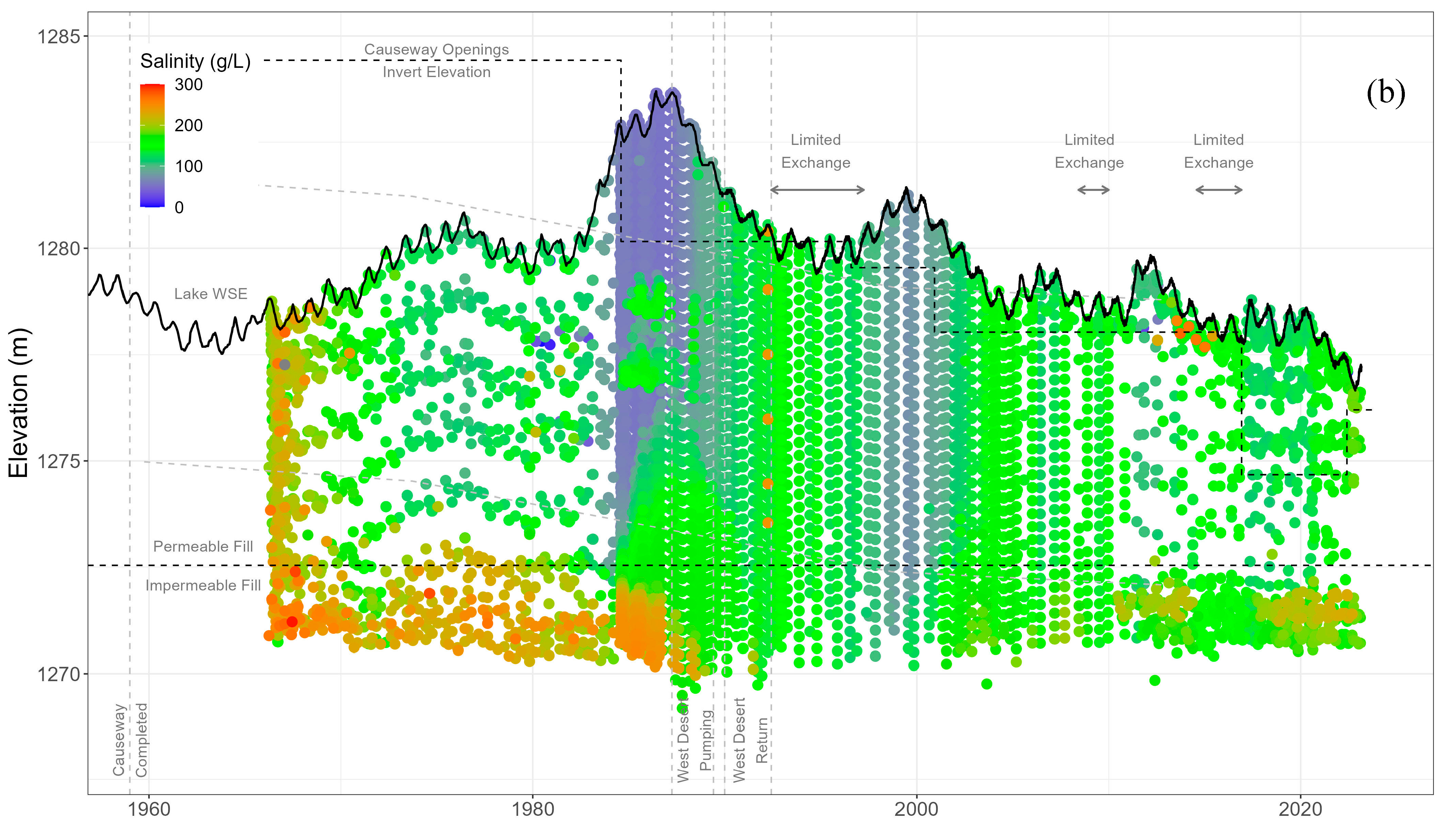
- How does salinity change within the lake?
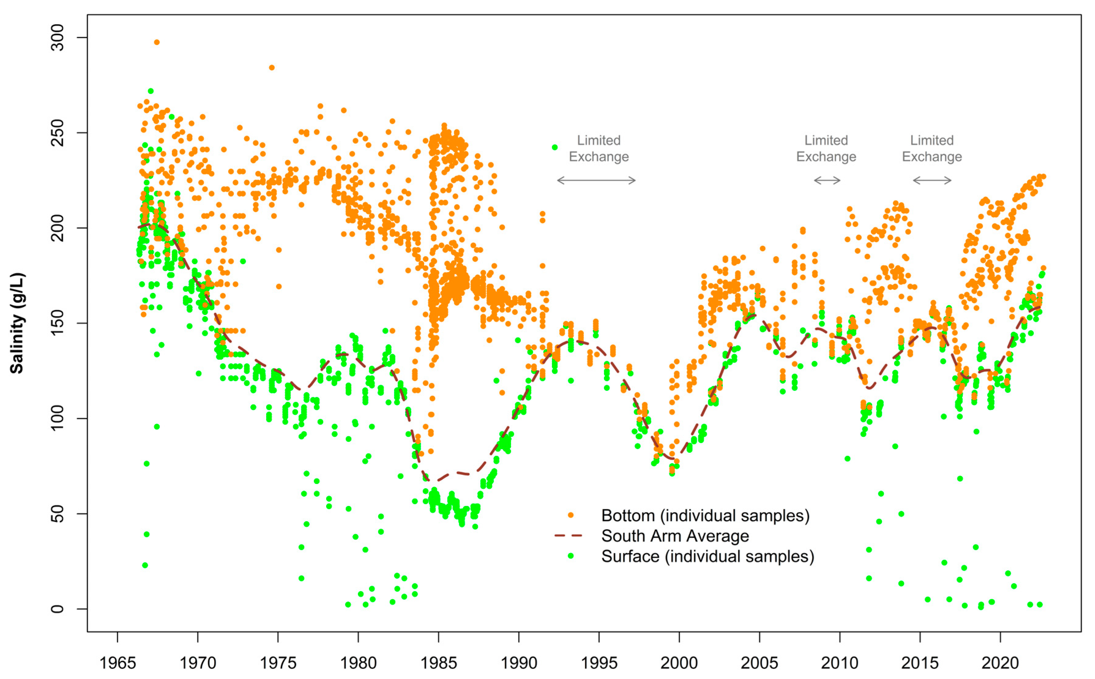
- How does the DBL fluctuate in time, space, and concentration?
- How does surface salinity relate to average salinity and the DBL?
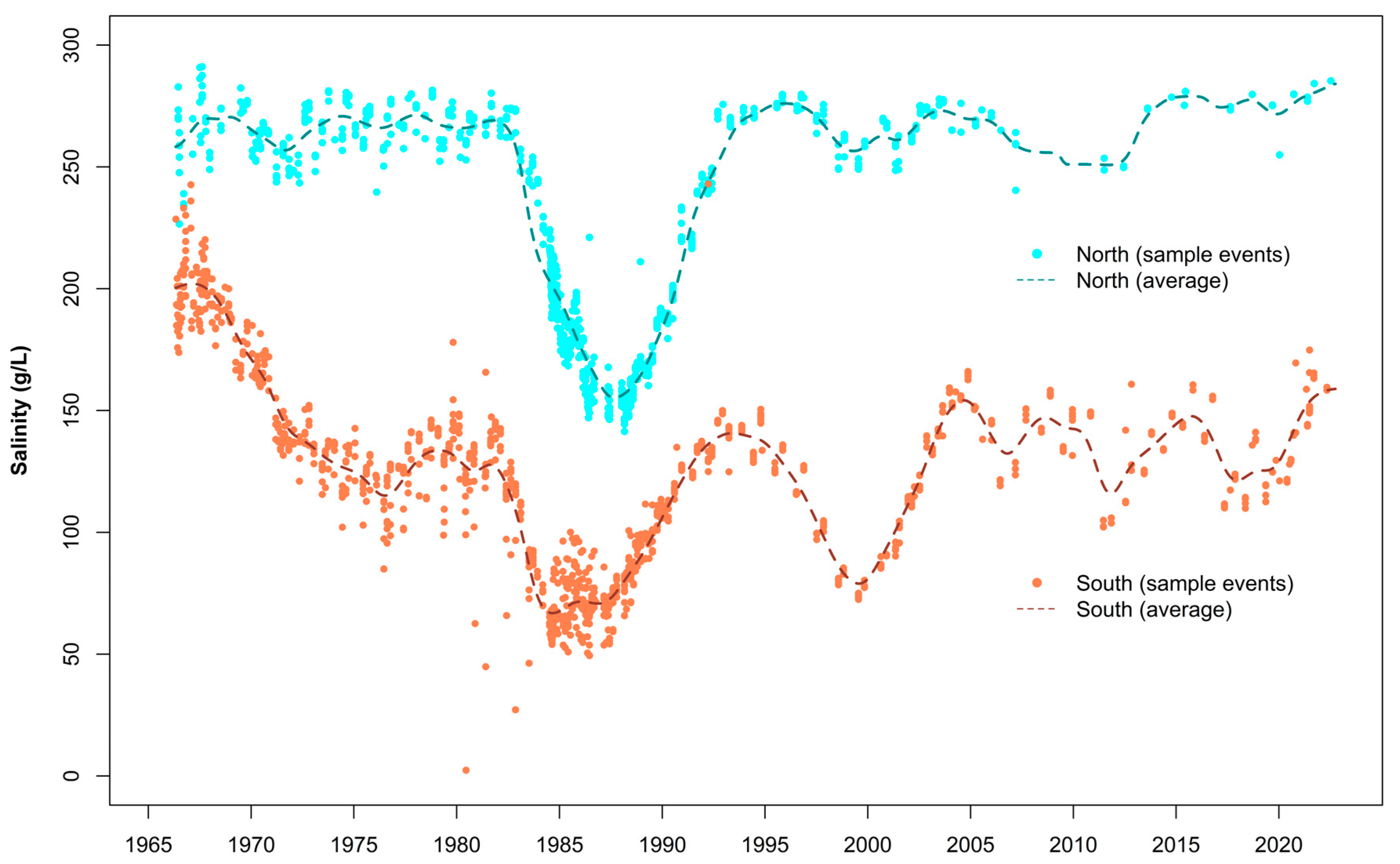
- How does salt move between the north and south arms?
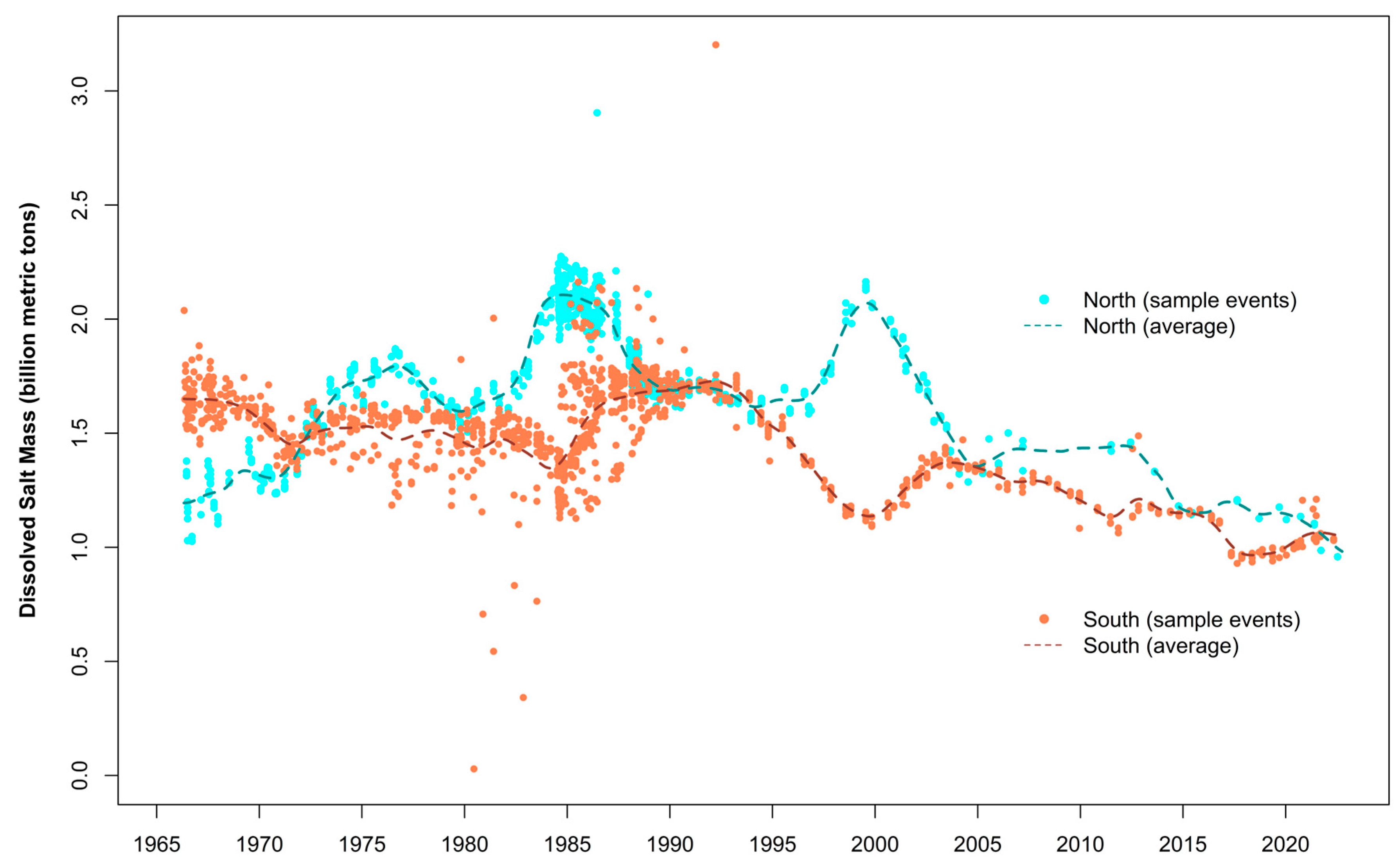
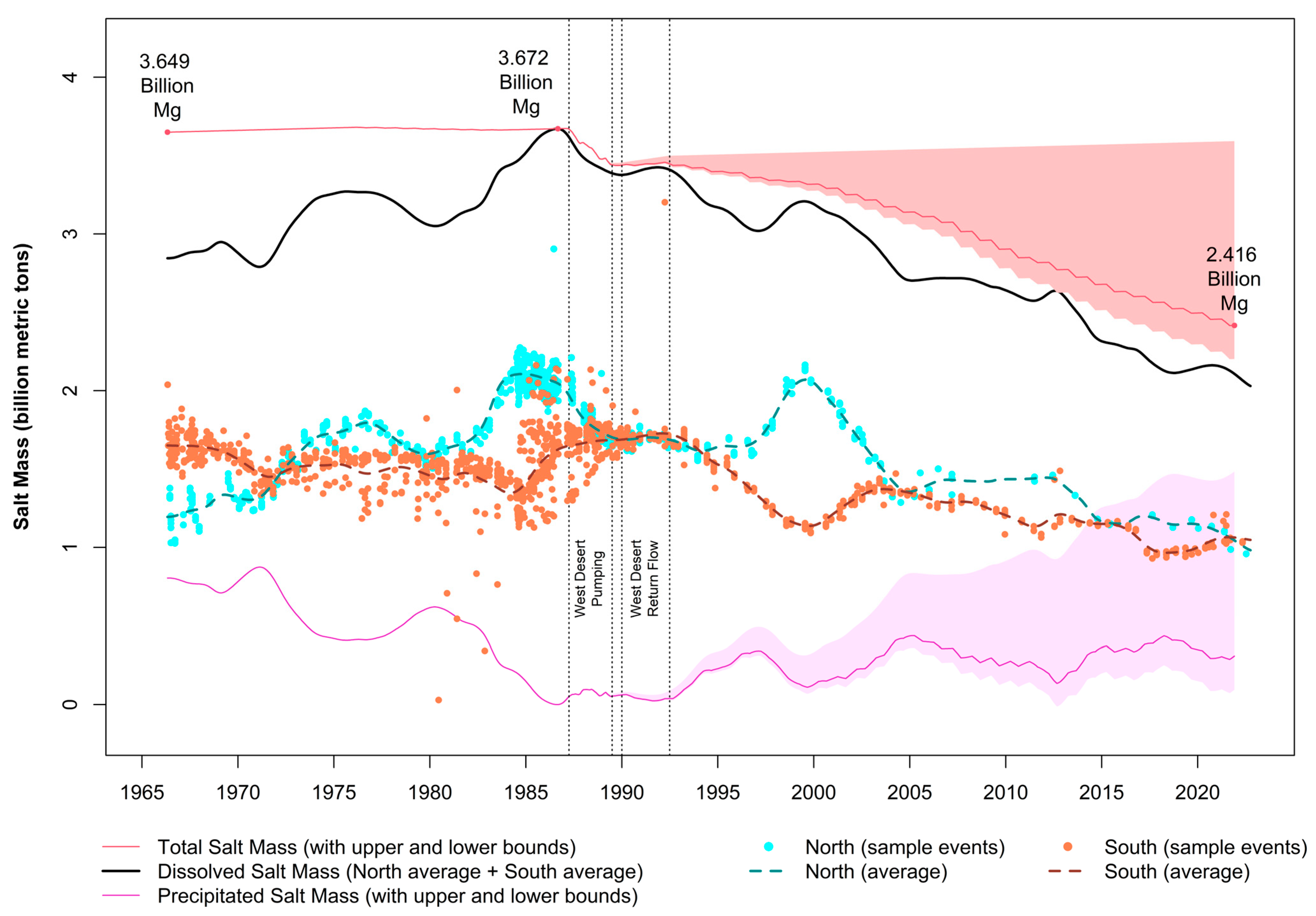
- How has the total salt mass changed over time?
2. Materials and Methods
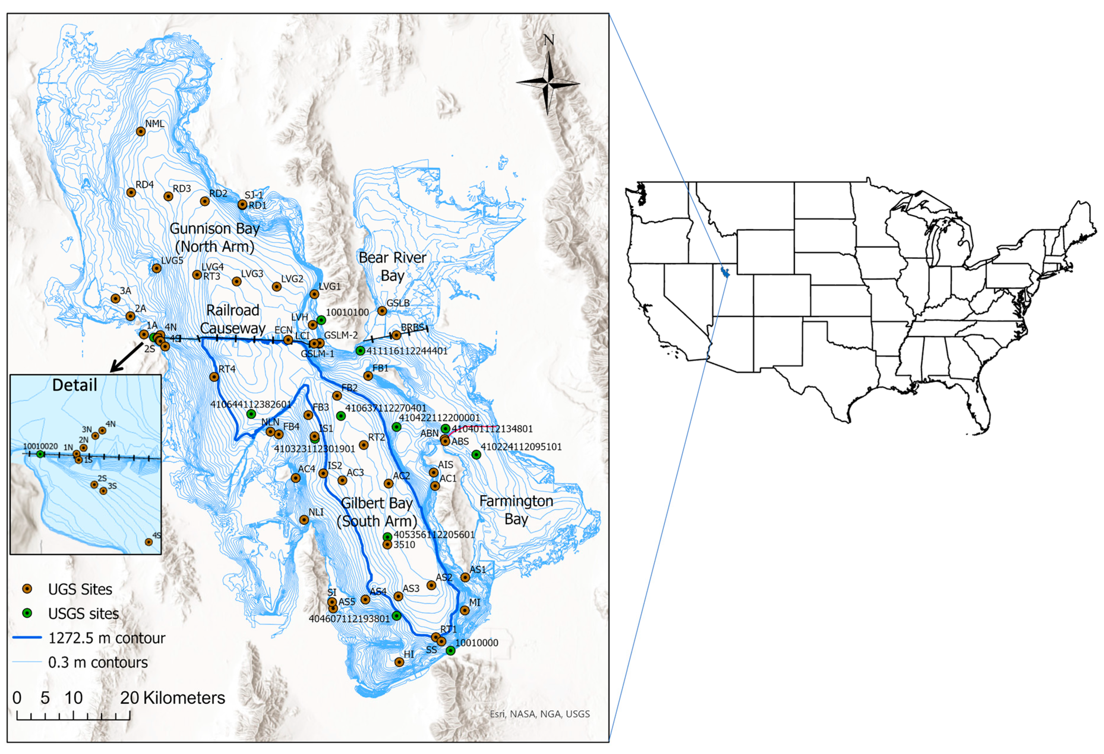
2.1. Bathymetry
2.2. Water Surface Elevation Data
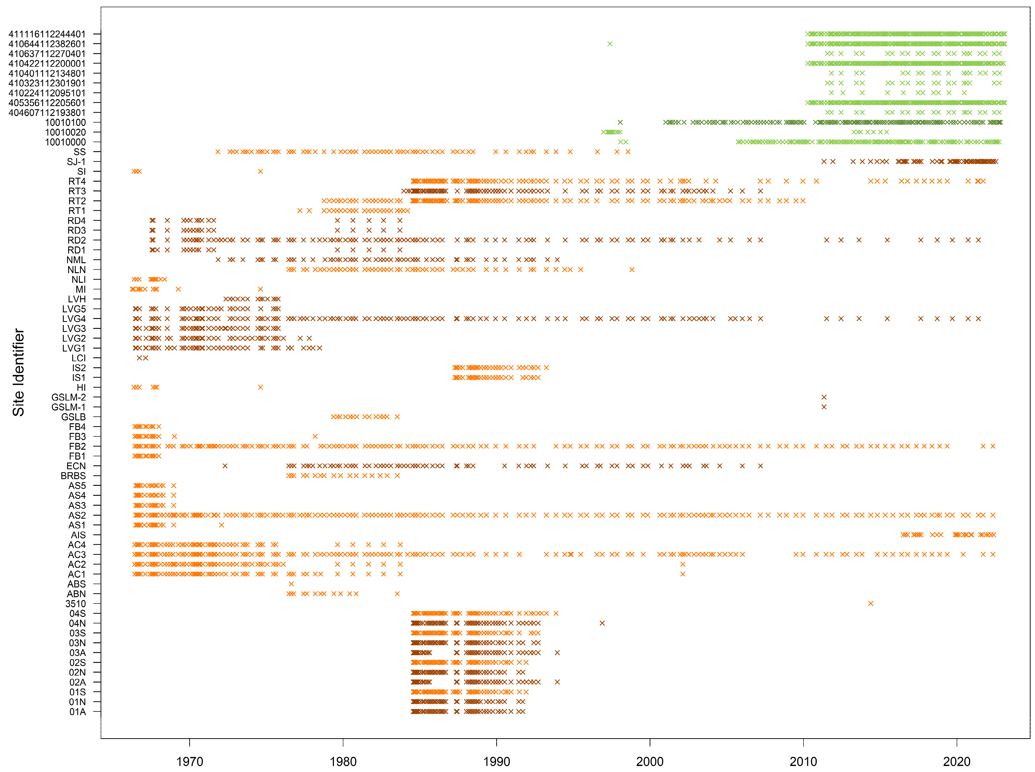
2.3. Water Sample Data
2.4. Salinity
- “Water Density: A measure of the mass (grams) per unit volume of water (cubic centimeter) including all solutes (g/cm3). Water density varies with temperature and total dissolved solids (TDS).”
- “Salinity: A measure of the concentration of all solutes dissolved in water. Solutes in GSL water are unique and difficult to accurately measure; GSL salinity is typically defined as the mass of dissolved solids (or TDS) in grams per liter of water (g/L).” [24] (p. 1)
2.5. Average Dissolved Salt Mass and Average Salinity
2.6. Total Salt Mass Calculations
- Salt mass increases due to annual inflow from rivers, wastewater, stormwater runoff, and groundwater estimated by Hahl [28] to be 3,175,000 metric tons (3,500,000 US tons; a US ton, sometimes referred to as a short ton, is 2000 lb or 0.907 metric tons; a metric ton is 1000 kg).
- Salt mass values for mineral pond leakage and return were estimated using volume equal to 25% of water rights withdrawal values following Utah Division of Water Resources estimates that net withdrawals are 75% of the water right, and salinity of the returning brine, which was assumed to be at a saturation density of approximately 1220 kg/m3 (1.22 g/cm3) [31] and a salinity of 275 g/L based on the Naftz et al. [16] equation of state (Equation (1)).
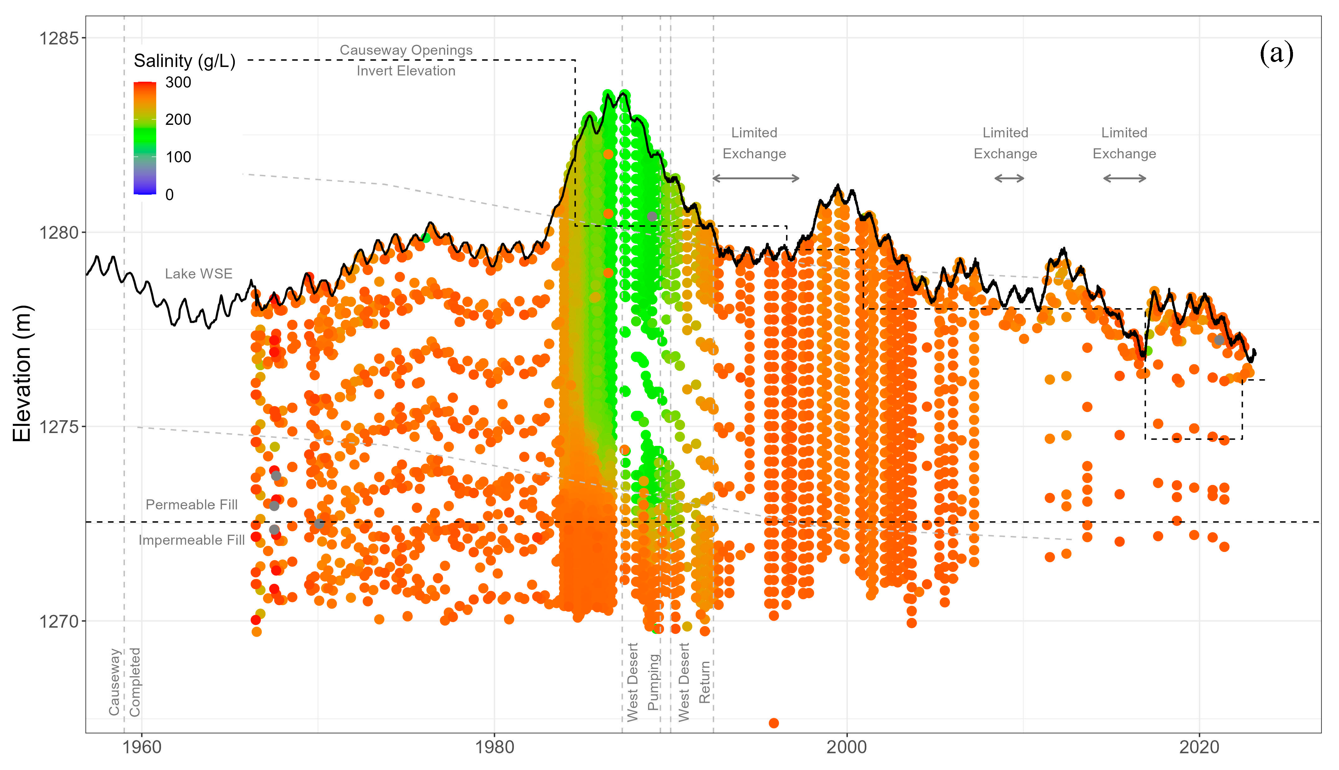
- The West Desert Pumping Project circulated water through the west desert pond from 1987 to 1989 and then drained water back to the lake from 1990 to 1992, bringing salt with it [5]. Loving et al. [5] report a net loss of 0.478 billion metric tons (0.527 billion US tons) of salt that precipitated and remained in the west desert. To reconcile our total dissolved salt mass calculations and not have the total salt mass go below the observed dissolved salt mass over the 1987–1992 time period, west desert pumping salt loss values reported by Loving et al. [5] were reduced by a factor of 0.4.
3. Results
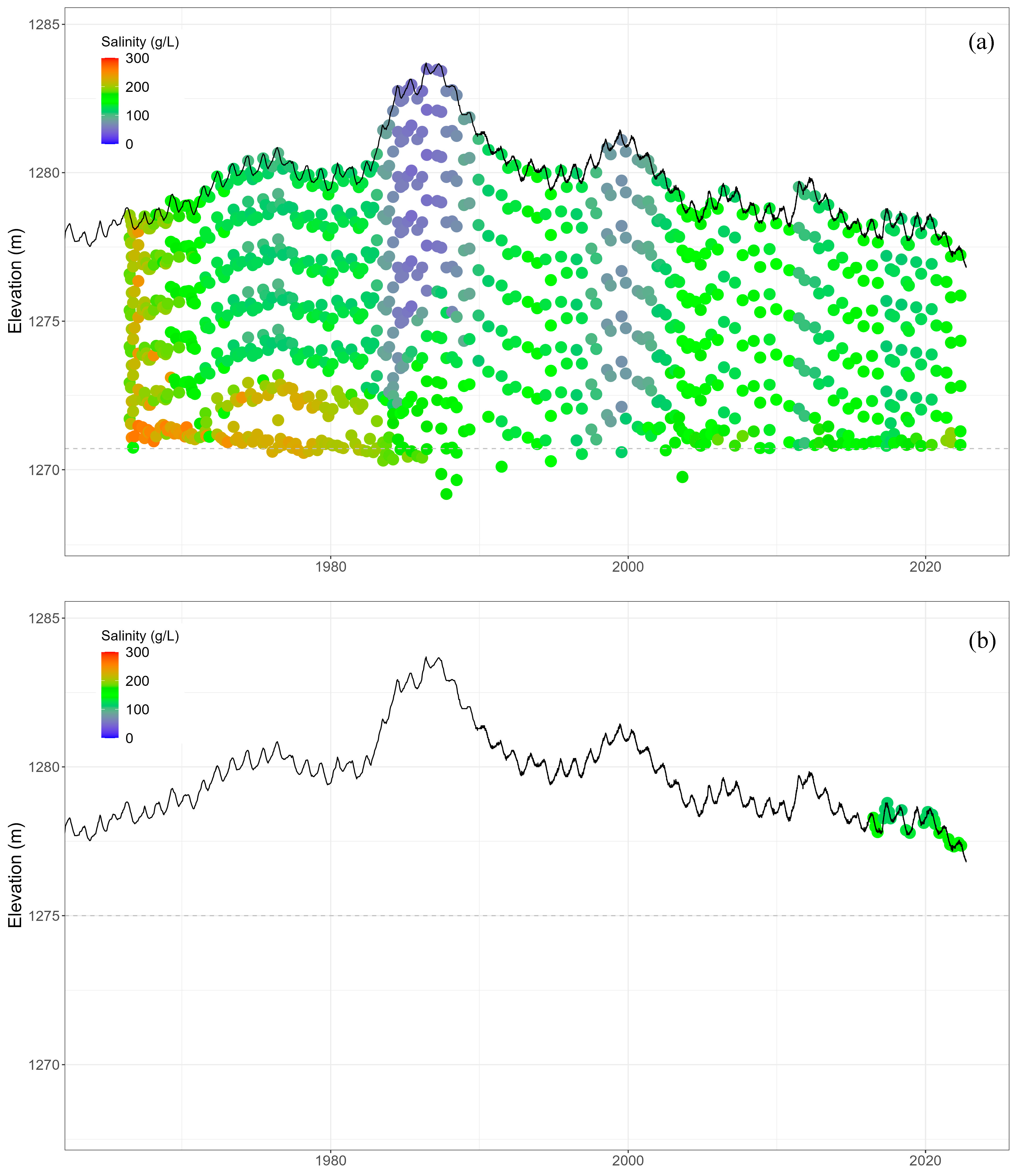
3.1. Salinity
3.2. Average Dissolved Salt Mass and Average Salinity
3.3. Total Salt Mass
4. Discussion
5. Conclusions
Supplementary Materials
Author Contributions
Funding
Data Availability Statement
Conflicts of Interest
References
- Jones, E.F.; Wurtsbaugh, W.A. The Great Salt Lake’s monimolimnion and its importance for mercury bioaccumulation in brine shrimp (Artemia franciscana). Limnol. Oceanogr. 2014, 59, 141–155. [Google Scholar] [CrossRef]
- Wurtsbaugh, W.A.; Berry, T.S. Cascading effects of decreased salinity on the plankton, chemistry, and physics of the Great Salt Lake (Utah). Can. J. Fish. Aquat. Sci. 1990, 47, 100–109. [Google Scholar] [CrossRef]
- Hassan, D.; Burian, S.J.; Johnson, R.C.; Shin, S.; Barber, M.E. The Great Salt Lake Water Level is Becoming Less Resilient to Climate Change. Water Resour. Manag. 2022, 1–24. [Google Scholar] [CrossRef]
- Utah Division of Forestry, Fire and State Lands (UDFFSL). Final Great Salt Lake Comprehensive Management Plan and Record of Decision; Utah Division of Forestry, Fire and State Lands: Salt Lake City, UT, USA, 2013; 391p. Available online: https://geodata.geology.utah.gov/pages/view.php?ref=8267 (accessed on 6 January 2023).
- Loving, B.L.; Waddell, K.M.; Miller, C.W. Water and Salt Balance of Great Salt Lake, Utah, and Simulation of Water and Salt Movement through the Causeway, 1987–98; U.S. Geological Survey: Salt Lake City, UT, USA, 2000. Available online: https://pubs.usgs.gov/wri/2000/4221/report.pdf (accessed on 12 August 2022).
- Tripp, T.G. Production of Magnesium from Great Salt Lake, Utah USA; Natural Resources and Environmental Issues: Article 10; Utah State University: Logan, UT, USA, 2009; Volume 15, Available online: https://digitalcommons.usu.edu/nrei/vol15/iss1/10 (accessed on 22 May 2012).
- White, J.S.; Null, S.E.; Tarboton, D.G. How do changes to the railroad causeway in Utah’s Great Salt Lake affect water and salt flow? PLoS ONE 2015, 10, e0144111. [Google Scholar] [CrossRef] [PubMed]
- Madison, R.J. Effects of a Causeway on the Chemistry of the Brine in Great Salt Lake, Utah; Water-Resources Bulletin; Utah Geological and Mineralogical Survey: Salt Lake City, UT, USA, 1970; Volume 14, 50p. Available online: https://ugspub.nr.utah.gov/publications/water_resources_bulletins/WRB-14.pdf (accessed on 1 March 2023).
- Naftz, D.; Angeroth, C.; Kenney, T.; Waddell, B.; Darnall, N.; Silva, S.; Perschon, C.; Whitehead, J. Anthropogenic influences on the input and biogeochemical cycling of nutrients and mercury in Great Salt Lake, Utah, USA. Appl. Geochem. 2008, 23, 1731–1744. [Google Scholar] [CrossRef]
- Valdes, C.; Black, F.J.; Stringham, B.; Collins, J.N.; Goodman, J.R.; Saxton, H.J.; Mansfield, C.R.; Schmidt, J.N.; Johnson, W.P. Total Mercury and Methylmercury Response in Water Sediment, and Biota to Destratification of the Great Salt Lake, Utah, USA. Environ. Sci. Technol. 2017, 51, 4887–4896. [Google Scholar] [CrossRef] [PubMed]
- Yang, S.; Johnson, W.P.; Black, F.J.; Rowland, R.; Rumsey, C.; Piskadlo, A. Response of density stratification, aquatic chemistry, and methylmercury to engineered and hydrologic forcings in an endorheic lake (Great Salt Lake, U.S.A.). Limnol. Oceanogr. 2019, 65, 915–926. [Google Scholar] [CrossRef]
- Wurtsbaugh, W.A.; Sima, S. Contrasting Management and Fates of Two Sister Lakes: Great Salt Lake (USA) and Lake Urmia (Iran). Water 2022, 14, 3005. [Google Scholar] [CrossRef]
- Diaz, X.; Naftz, D.L.; Johnson, W.P. Selenium Mass Balance in the Great Salt Lake, Utah. Sci. Total Environ. 2009, 407, 2333–2341. [Google Scholar] [CrossRef] [PubMed]
- Diaz, X.; Johnson, W.P.; Fernandez, D.; Naftz, D.L. Size and Elemental Distributions of Nano- to Micro- Particulates in the Geochemically-stratified Great Salt Lake. Appl. Geochem. 2009, 24, 1653–1665. [Google Scholar] [CrossRef]
- Brown, P.D.; Bosteels, T.; Marden, B.T. Salt load transfer and changing salinities across a new causeway breach in Great Salt Lake: Implications for adaptive management. Lakes Reserv. Sci. Policy Manag. Sustain. Use 2023, 28, e12421. [Google Scholar] [CrossRef]
- Naftz, D.L.; Millero, F.J.; Jones, B.F.; Green, W.R. An Equation of State for Hypersaline Water in Great Salt Lake, Utah, USA. Aquat. Geochem. 2011, 17, 809–820. [Google Scholar] [CrossRef]
- Baskin, R.L.; Allen, D.V. Bathymetric Map of the South Part of Great Salt Lake, Utah: U.S. Geological Survey Scientific Investigations Map 2894; USGS: Reston, VA, USA, 2005. Available online: https://pubs.usgs.gov/sim/2005/2894/ (accessed on 1 March 2023).
- Baskin, R.L.; Turner, J. Bathymetric Map of the North Part of Great Salt Lake, Utah: U.S. Geological Survey Scientific Investigations Map 2006–2954; USGS: Reston, VA, USA, 2006. [CrossRef]
- Baskin, R.L. Farmington Bay Contours in 2009 and Modified by BIO-WEST in 2010, Including Minor Contour Manipulation and the Introduction of a 1280 Meter (4200 Foot) Contour at the South End of the Bay. Personal communication. 2010. [Google Scholar]
- Hansen & Associates. Bear River Bay Survey in 2009 under a Contract with BIO-WEST. Personal communication. 2010.
- ESRI. ArcGIS Desktop: Release 10; Environmental Systems Research Institute: Redlands, CA, USA, 2015. [Google Scholar]
- Tarboton, D. Great Salt Lake Bathymetry. HydroShare. 2017. Available online: http://www.hydroshare.org/resource/582060f00f6b443bb26e896426d9f62a (accessed on 1 March 2023).
- Tarboton, D. Great Salt Lake Area Volume Data. HydroShare. 2017. Available online: http://www.hydroshare.org/resource/89125e9a3af544eab2479b7a974100ba (accessed on 1 March 2023).
- Great Salt Lake Salinity Advisory Committee. Standard Operating Procedure—Great Salt Lake Water Density Measurement and Salinity Calculation; Utah Geological Survey Open-File Report 728; Great Salt Lake Salinity Advisory Committee: Salt Lake City, UT, USA, 2020; 6p. [CrossRef]
- Spieweck, F.; Bettin, H. Review: Solid and liquid density determination. Tech. Mess. 1992, 59, 285–292. [Google Scholar] [CrossRef]
- Mohammed, I.N.; Tarboton, D.G. An examination of the sensitivity of the Great Salt Lake to changes in inputs. Water Res. Res. 2012, 48, W11511. [Google Scholar] [CrossRef]
- R Core Team. R: A Language and Environment for Statistical Computing; R Foundation for Statistical Computing: Vienna, Austria, 2012; Available online: http://www.R-project.org/ (accessed on 1 March 2023).
- Hahl, D.C. Dissolved-Mineral Inflow to Great Salt Lake and Chemical Characteristics of the Salt Lake Brine: Summary for Water Years 1960, 1961, and 1964; Water-Resources Bulletin 10; Utah Geological Survey: Salt Lake City, UT, USA, 1968; 35p.
- Utah Division of Water Rights. WUSEVIEW Water Records/Use Information Viewer. Available online: https://waterrights.utah.gov/cgi-bin/wuseview.exe (accessed on 28 February 2023).
- Merck, M.; Tarboton, D. Great Salt Lake Mineral Extraction Water Withdrawals. HydroShare. 2023. Available online: http://www.hydroshare.org/resource/46b98820b7214850aadf6fa60c9bc1d1 (accessed on 8 March 2023).
- Rupke, A.; Jagnieki, E. The Significance of Great Salt Lake’s North Arm on Lake Salinity; Survey Notes; Utah Geological Survey: Salt Lake City, UT, USA, 2021. Available online: https://ugspub.nr.utah.gov/publications/survey_notes/snt53-1.pdf (accessed on 1 March 2023).
- Rasmussen, M.; Dutta, S.; Neilson, B.T.; Crookston, B.M. CFD Model of the Density-Driven Bidirectional Flows through the West Crack Breach in the Great Salt Lake Causeway. Water 2021, 13, 2423. [Google Scholar] [CrossRef]
- Waddell, K.M.; Bolke, E.L. The Effects of Restricted Circulation on the Salt Balance of Great Salt Lake, Utah; Water-Resources Bulletin; Utah Geological Survey: Salt Lake City, UT, USA, 1973; Volume 18, p. 54. Available online: https://ugspub.nr.utah.gov/publications/water_resources_bulletins/WRB-18.pdf (accessed on 1 March 2023).
- Wold, S.R.; Thomas, B.E.; Waddell, K.M. Water and Salt Balance of Great Salt Lake, Utah, and Simulation of Water and Salt Movement through the Causeway; Water Supply Paper 2450: 1–64; US Geological Survey: Salt Lake City, UT, USA, 1997. [CrossRef]
- Bioeconomics, Inc. Economic significance of the Great Salt Lake to the State of Utah. Prepared for State of Utah Great Salt Lake Advisory Council. 2012. Available online: https://documents.deq.utah.gov/water-quality/standards-technical-services/great-salt-lake-advisory-council/Activities/DWQ-2012-006863.pdf (accessed on 1 March 2023).
- Western Hemisphere Shorebird Reserve Network (WHSRN). Conserving Shorebirds and Their Habitat through a Network of Key Sites across the Americas. Available online: www.whsrn.org (accessed on 1 March 2023).
- Aldrich, T.W.; Paul, D.S. Avian ecology of Great Salt Lake. In Great Salt Lake: An Overview of Change; Gwynn, J.W., Ed.; Utah Department of Natural Resources: Salt Lake City, UT, USA, 2002; pp. 343–374. [Google Scholar]
- Rupke, A. (Utah Geological Survey, Salt Lake City, Utah, USA). Personal communication. 2022. [Google Scholar]


| Mass Contribution | 1966–1986 (20 Years) | 1986–2021 (35 Years) |
|---|---|---|
| River, Groundwater and Other Inputs | 0.065 | 0.112 |
| West Desert Project | - | −0.191 |
| Mineral Extraction North Arm Withdrawal | - | −1.277 |
| Mineral Extraction North Arm Return | - | 0.346 |
| Mineral Extraction South Arm Withdrawal | −0.099 | −0.511 |
| Mineral Extraction South Arm Return | 0.057 | 0.265 |
Disclaimer/Publisher’s Note: The statements, opinions and data contained in all publications are solely those of the individual author(s) and contributor(s) and not of MDPI and/or the editor(s). MDPI and/or the editor(s) disclaim responsibility for any injury to people or property resulting from any ideas, methods, instructions or products referred to in the content. |
© 2023 by the authors. Licensee MDPI, Basel, Switzerland. This article is an open access article distributed under the terms and conditions of the Creative Commons Attribution (CC BY) license (https://creativecommons.org/licenses/by/4.0/).
Share and Cite
Merck, M.F.; Tarboton, D.G. The Salinity of the Great Salt Lake and Its Deep Brine Layer. Water 2023, 15, 1488. https://doi.org/10.3390/w15081488
Merck MF, Tarboton DG. The Salinity of the Great Salt Lake and Its Deep Brine Layer. Water. 2023; 15(8):1488. https://doi.org/10.3390/w15081488
Chicago/Turabian StyleMerck, Madeline F., and David G. Tarboton. 2023. "The Salinity of the Great Salt Lake and Its Deep Brine Layer" Water 15, no. 8: 1488. https://doi.org/10.3390/w15081488
APA StyleMerck, M. F., & Tarboton, D. G. (2023). The Salinity of the Great Salt Lake and Its Deep Brine Layer. Water, 15(8), 1488. https://doi.org/10.3390/w15081488