Article

Assessment of Water Conservation Services Based on the Method of Integrating Hydrological Observation Data According to Different Ecosystem Types and Regions

Satellite Application Center for Ecology and Environment, Ministry of Ecology and Environment of the People’s Republic of China, Beijing 100094, China
*
Author to whom correspondence should be addressed.
Water 2023, 15(8), 1475; https://doi.org/10.3390/w15081475
Submission received: 18 March 2023 / Revised: 5 April 2023 / Accepted: 7 April 2023 / Published: 10 April 2023

Abstract

:
Water conservation is an essential indicator of the hydrological regulation capacity of terrestrial ecosystems. At the regional scale, the water conservation capacity of an ecosystem is typically assessed using the water balance model (WBM). However, the estimation of the runoff depth relies heavily on rainfall data and the ecosystem runoff coefficient look-up table, which introduces uncertainties in the assessment results. To address this issue, this study constructed a new method for quantifying the spatiotemporal distribution pattern of runoff depth based on the ecosystem type and regional spatial heterogeneity characteristics using runoff observation data from hydrological observation stations. We use this new method to evaluate the water conservation capacity of the ecosystem on a regional scale and compare and analyze the differences between the new and old methods in terms of connotation, data format, and evaluation results. Finally, we discuss the advantages and potential applications of the new method.

1. Introduction

Water conservation and soil conservation are commonly used indicators to assess ecosystem regulating services from the perspective of “water” and “soil”. While soil conservation has a relatively clear definition and calculation models, such as the Revised Universal Soil Loss Equation (RUSLE) and the Revised Wind Erosion Equation (RWEQ), for indirectly assessing ecosystem soil conservation services from hydraulic erosion and wind erosion [1,2]. However, there is still no unified concept and mathematical expression of water conservation in the academic community. This is mainly due to the fact that the purpose of studies mainly include water storage and water use, and the corresponding evaluation methods focus on the ecosystem’s ability to store water or generate runoff. In general, in the process of eco-hydrology, an increase in water storage in the ecosystem means a decrease in runoff production capacity [3,4,5,6,7]. As such, different assessment and quantification methods often bring confusion to regional ecological protection and decision making. Despite this, quantifying water conservation or storage capacity of an ecosystem is necessary and common in the assessment of water conservation, regardless of the ecosystem service or the functional characteristics of the ecosystem itself.
In general, an increase in water storage in the ecosystem means a decrease in runoff production capacity, which is the focus of research on the eco-hydrological mechanism, water resource utilization, flood control, and drought relief projects [8,9,10,11]. Conversely, research on ecological function assessment aimed at regional ecological protection and ecosystem restoration focuses more on describing the role of the ecosystem in water storage [12,13,14,15]. Therefore, a clear definition and standardized mathematical expression of water conservation would be valuable in providing a more accurate and comprehensive assessment of water conservation and management.
Currently, the water balance model (WBM) has the ability to accurately quantify the input (rainfall) and output (evaporation and runoff) of an ecosystem at the regional and watershed scales due to its black box nature. This allows for comprehensive analysis of the characteristics and processes of the flow and storage of ecosystem water, making the WBM a preferred model for ecosystem services and functions from both conservation and runoff production perspectives [16,17,18]. Moreover, the WBM not only benefits the research field, but also directly supports the administrative work of national and regional ecological protection policies. It has become a common method of ecosystem assessment and even restricts the implementation of projects in the form of standards and specifications, such as in the assessment of forest ecosystem services, regular remote sensing investigation and assessment of national ecological status in China, the spatial planning of national land in China, the delimitation of ecological conservation redline in China [19,20,21,22,23,24], etc.
In the application of the water balance model, obtaining precise runoff data that match the data format, spatial scale, and resolution at the same time is challenging. Precipitation and evapotranspiration data sets obtained through site monitoring or satellite remote sensing monitoring are objective and consistent in time and space. However, the flow data observed by hydrological stations, which are often distributed along the river, cannot directly establish a quantitative relationship with the ecosystem, as they represent a comprehensive reflection of the basin runoff. Moreover, difficulties in data sharing of hydrological station observation flow data impede the establishment of a spatial data set of runoff depth. Thus, obtaining runoff spatial distribution data is crucial for assessing the water conservation of regional ecosystems using the WBM. Generally, the precipitation and runoff coefficient of different ecosystem types are used to estimate the temporal and spatial distribution of runoff depth. This method has found widespread application in the study of ecosystem water conservation service assessment [13,19,20,21,22,23,24].
The runoff coefficient denotes the proportion of runoff to precipitation over a specified period, influenced by various factors, such as topography, watershed morphology, vegetation, and soil type [25]. It is a comprehensive metric that reflects the interplay between natural geographical factors and the rainfall–runoff relationshipSmall-scale investigations of the runoff coefficient focus on municipal construction, flood control engineering, drought relief, water and soil loss mechanisms, and drainage irrigation in small watersheds [26,27,28,29,30,31,32]. The use of remote sensing data allows for the development of spatial distribution grid data sets of ecosystem types with relative ease. The integration of experimental observations and ecological hydrological model research can aid in the acquisition of runoff coefficients for various ecosystem types. Consequently, the creation of a lookup table matching ecosystem type values with corresponding runoff coefficients can generate a spatial distribution grid data set of runoff coefficients using the lookup table method (LTM). This technique has been implemented in scientific research and technical guidance documents for evaluating water conservation services at the national and regional level [33,34,35,36]. Several case studies and methodological studies have confirmed its effectiveness [12,13,15,20,21,22,23]. Although variations exist among the lookup tables utilized in these studies, there are no fundamental differences or improvements in essence. The differences mainly stem from subjective literature review differences and varying research objectives among researchers. For instance, references [12,13] have different runoff coefficient values for evergreen broadleaf forests, specifically 2.67 and 4.65, respectively, while reference [22] presents additional runoff coefficient values for farmland and construction land.
The lookup table method (LTM) is a widely utilized approach for acquiring runoff coefficients at a regional scale. However, this method is associated with notable deficiencies in three main areas. Firstly, due to the absence of actual hydrological observation data, the results of water conservation assessments are not representative of the true hydrological regulation capacity of the ecosystem. Secondly, the physical and geographical characteristics of the basin cannot be accurately described, as the runoff coefficient obtained from the LTM fails to consider the basin morphology and physical geographical features, resulting in the masking of differences in the runoff production capacity of the same ecosystem type in different watersheds. Thirdly, the lack of time-varying information is a significant limitation, as the runoff coefficient is considered a constant, neglecting the changes in vegetation growth, while the ecosystem type remains constant. These changes could be critical in determining the impact of regional climate change and human activities on the ecosystem [37]. Despite the widespread use of the LTM, there is a conspicuous paucity of literature on water conservation assessment studies that can address its limitations and offer alternative approaches for quantifying runoff depth.
In this investigation, we have developed a novel research framework termed “different regions, different types” for the acquisition and spatialization of runoff data. Specifically, we have introduced the runoff observation method (ROM), which utilizes data collected by hydrological stations within a specific basin to obtain spatiotemporal distribution data of runoff depth, enabling regional water conservation assessment. The ROM method involves the integration of runoff observation data, soil data, and ecosystem classification data, followed by the use of GIS spatial analysis to integrate the spatial information of different soil regions and ecosystem types on the pixel scale. Moreover, we have employed a simple and effective area-weighting method to directly derive the runoff depth spatial distribution data set consistent with the ecosystem classification in spatial scale, data format, and resolution by combining the real flow information observed by the watershed hydrological stations. We have further utilized the water balance model to calculate the annual water conservation amount and obtain the annual runoff coefficient spatial distribution data set. To demonstrate the effectiveness of our proposed method, we have compared and analyzed the results of runoff depth and water conservation based on the precipitation and runoff coefficient lookup table.

2. Materials and Methods

2.1. Study Area

The water balance model is a comprehensive tool that can provide insights into the water flow and storage characteristics within a basin to ensure that the input of water is mainly from rainfall and runoff at the inlet of the basin and the consumption of water is mainly evapotranspiration and runoff at the outlet of the basin. To this end, we selected a representative basin in the upper reaches of the Yellow River (as shown in Figure 1) and ensured that there was a national hydrological station located at both the inlet and outlet of the basin. By assuming that the impact of human activities, such as industry and agriculture, was negligible, we could focus on understanding the natural characteristics of the ecosystem, the geography itself, and how they contribute to water storage and runoff production.
The study area on the Yellow River (Figure 1) included Jimai Station as the inlet and Lanzhou Station as the outlet, which are both national hydrological stations. This region is situated at the intersection of the Qinghai–Tibet Plateau and the Loess Plateau, with an average elevation of over 3400 m, and it is characterized by meadow grassland and natural wetland. It serves as a crucial water source for the Yellow River basin, consisting of the main stream of the Yellow River and four primary tributaries: Huangshui, Baihe, Heihe, and Taohe. The basin is mainly dominated by animal husbandry, and the density of industry and irrigated agriculture is relatively low. The basin boundary and the hydrological stations locations were manually verified and corrected using the satellite remote sensing images with a resolution of more than 2 m, combined with the existing boundary data, to ensure their accuracy [38].

2.2. Technical Framework

The technical process comprised five primary steps, as depicted in Figure 2.
Firstly, satellite remote sensing imagery was utilized to generate ecosystem type data for the study area, as detailed in Section 2.3.1. In Section 2.3.2, the relevant literature is reviewed to gather information on the runoff coefficient values for various ecosystem types. Additionally, the Harmonized World Soil Database version 1.2 (HWSD) was utilized to extract the curve number (CN) values associated with different combinations of hydraulic soil groups (HSG).
Secondly, as described in Section 2.3.2, tables containing information on the runoff coefficient and curve number (CN) values for various ecosystem types were combined with the ecosystem classification to construct runoff index spatial data based on ecosystem type and HSG. The comprehensive runoff index raster data set of “different regions, different types” was synthesized using equal weighting to indicate the runoff generation capacity of each grid on a pixel scale. A schematic diagram of the logical principle is presented in Figure 3.
Thirdly, the spatial distribution of runoff depth was generated by allocating the runoff observed by hydrological stations in the comprehensive runoff index spatial raster data using the area-weighted method, as outlined in Section 2.3.3 and Section 2.4.1.
Fourthly, combining the rainfall obtained by meteorological station interpolation and the evapotranspiration product data set obtained by satellite remote sensing, the spatial distribution data set of water conservation capacity was calculated in accordance with the WBM, as expounded in Section 2.4.2.
Finally, the runoff coefficient raster data sets were computed from the runoff depth and rainfall data sets, as detailed in Section 2.4.3.

2.3. Data Sources and Processing

2.3.1. Ecosystem Types Data

In conformity with the ecosystem classification system prescribed by the national ecological environment industry standard document [39], five phases of ecosystem classification data for the years 2000, 2005, 2010, 2015, and 2020 were procured by mean of human–computer interactive interpretation of Landsat series satellite images, with a spatial resolution of 30 m. The accuracy of the interpretation of the aggregated classes was confirmed to have reached 94.3% [40].

2.3.2. Determine Runoff Index by Ecosystem Type and Hydrological Soil Group (HSG)

Firstly, the meta-analysis approach was implemented to extensively gather relevant literature, enabling the acquisition of the runoff coefficient data of diverse ecosystem types present in the study area or in areas geographically similar. The obtained data were utilized to construct the runoff coefficient table (Table 1). The hydrological soil group (HSG) and ecosystem types were employed to extract the curve number (CN) values from the HWSD database (Table 2) [34].
Secondly, to capture the basin’s unique characteristics and gauge the comparative runoff capacity of diverse ecosystems, this investigation postulates that the minimum runoff coefficient for any given ecosystem is equal to 1, thereby serving as the reference value for the ecosystem runoff index. Computation of the ecosystem runoff index (Rit) was conducted by dividing the ecosystem’s runoff coefficient by the reference value, using the division method (refer to Formula (1) and Table 1). Analogously, for each combination of HSG and ecosystem type, the runoff index of oil (Ris) was derived using Formula (2).
R i t j = R c j / R c min
In this formula, R i t j is the runoff index of type j , R c is the runoff coefficient of type j , and   R c min is the minimum value of the runoff coefficient of all ecosystem types.
R i s j , K = C N j , K / C N min
In this formula, R i s j , K is the runoff index of the value of HSG classification K of type j , C N j , K is the CN value of HSG classification K of type j , and C N min is the minimum value of CN value of all HSG classification and ecosystem types.
Thirdly, based on the ecosystem type data, the two runoff indexes are added and operated in an equal weight manner (see Formula (3)) pixel by pixel to generate the comprehensive runoff index (Ri) raster data set.
R i j , K = 0.5 × R i t j + 0.5 × R i s j , K
In this formula, R i j , K is a comprehensive runoff index of the value of HSG classification K of type j .

2.3.3. Hydrological Station Data and Processing

The runoff data used in this study were obtained from the Annual Hydrological Report of P. R. China [55], which includes daily observation data from 2001 to 2020 at the inlet and outlet hydrological stations of the basin. These data were summarized as annual values. The basin’s total runoff was calculated as the difference between the flow at the outlet hydrological station and the flow at the inlet hydrological station, as per Formula (4).
Δ R = R o u t l e t R i n l e t
In this formula, Δ R is the total runoff in the basin, R o u t l e t is the annual flow of the outlet hydrological station (Lanzhou station), and R i n l e t is the annual flow of the inlet hydrological station (Jimai station).

2.3.4. Precipitation Data and Interpolation

The precipitation was from the observation data of 251 meteorological stations provided by the China Meteorological Administration. The ANUSPLIN interpolation software was used to generate the annual precipitation raster data set with a spatial resolution of 500 m from 2000 to 2020.

2.3.5. Evapotranspiration Data and Processing

The annual evapotranspiration data set with a spatial resolution of 500 m and a time range of 2000–2020 was generated using the MODIS standard products (MOD16A2). The data were derived by synthesizing the annual values [56].

2.4. Methods

2.4.1. Runoff Depth Calculation

The methodology comprises a series of steps, beginning with the determination of the annual total watershed runoff ( Δ R ) by following the procedures outlined in Section 2.3.3. Subsequently, the sum of all pixel values (S) of the comprehensive runoff index grid data was calculated. Thereafter, the runoff value ( Δ r ) corresponding to the annual comprehensive runoff index per unit was calculated through division operations. Finally, the annual grid data set of runoff depth was obtained by multiplying the annual value ( Δ r ) with the comprehensive runoff index grid data. This approach, referred to as the runoff observation method (ROM), involves the redistribution of the actual runoff values observed by hydrological stations to each pixel. Moreover, as the spatial resolution of the comprehensive runoff index grid data inherits the attributes of ecosystem type data, the spatial resolution of the resulting runoff depth grid data set remains at 30 m.
To enable a comparison with the lookup table method (LTM), we generated an annual runoff depth raster data set with a spatial resolution of 500 m by using the runoff coefficient table (Table 1) and precipitation data.

2.4.2. Water Conservation Calculation

The annual water conservation amount is calculated according to Formula (5).
W R = P E R
In this formula, W R is the water conservation amount, P is the annual precipitation, and R is the annual evapotranspiration.
Similarly, we calculated the annual water conservation capacity based on the two methods (ROM and LTM) for comparative analysis.

2.4.3. Runoff Coefficient Calculation

Based on the runoff observation method (ROM), the annual runoff coefficient raster data set can be directly calculated using Formula (6).
R c = R / P
In this formula, R c is the runoff coefficient, R is the runoff depth, and P is the annual precipitation.

2.4.4. Trend Analysis Method

The Mann–Kendall (MK) trend test with Sen slope estimation was used to analyze the time series changes in pixel scale [57,58,59]. It mainly includes the temporal variation characteristics of runoff depth and water conservation.

3. Results

3.1. Change in Runoff Depth

3.1.1. Spatial Variation

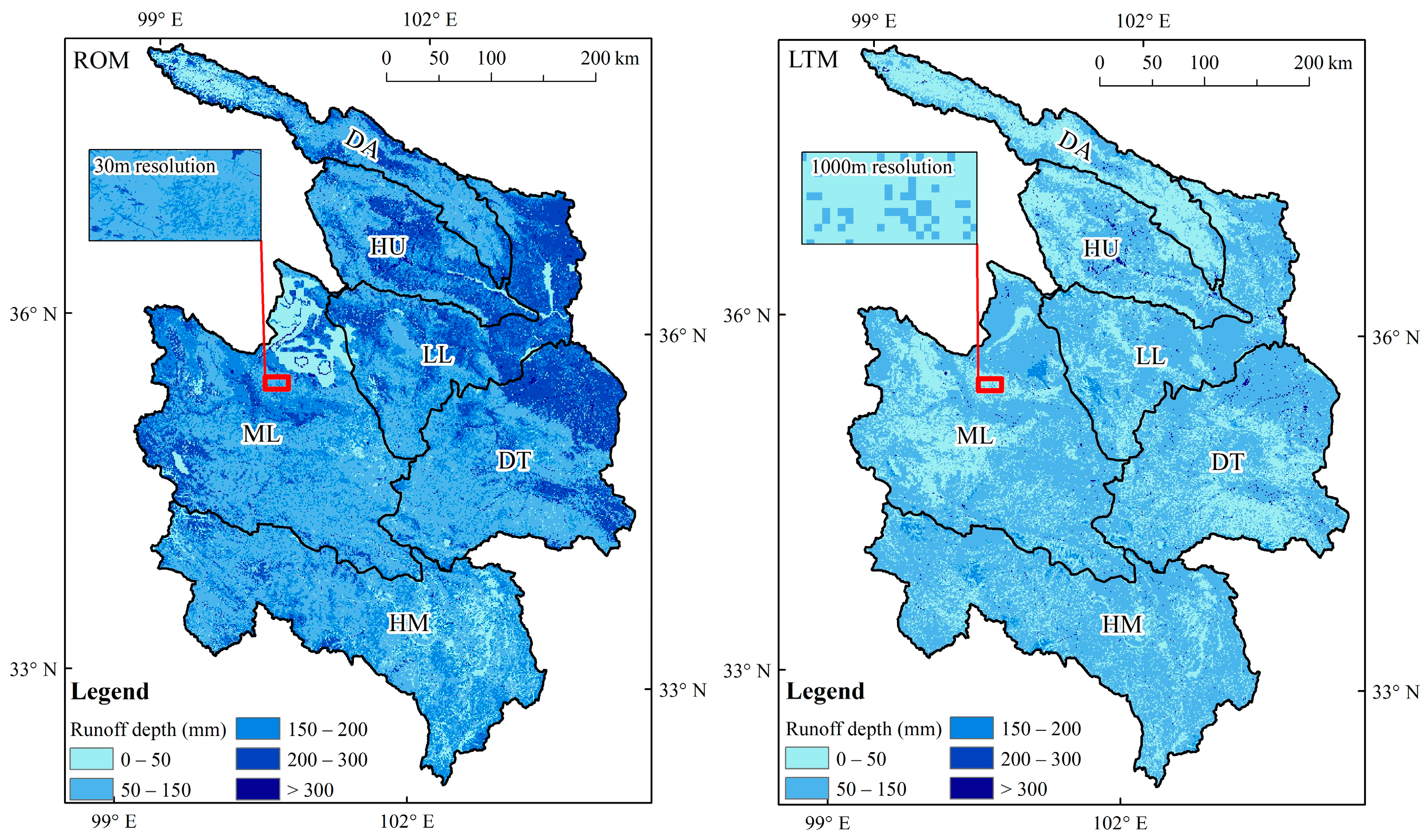
The average runoff depth from 2000 to 2020 was calculated by two methods (ROM and LTM), respectively (Figure 4). The spatial differentiation characteristics were more prominent in the ROM results. The runoff depth area (>200 mm) was mainly located in the northeast of the basin (HU LL and DT), while the low runoff depth area (<150 mm) area was in the northwest and west (DA ML and HM). The LTM results displayed a similar spatial pattern, but the spatial heterogeneity was not apparent. The average runoff depth computed by ROM was 146.08 mm, significantly higher than the average value of 61.66 mm calculated by LTM. The ROM approach only required the ecosystem classification and soil survey data, allowing a finer spatial resolution of 30 m for the runoff depth spatial data. In contrast, the LTM method relied on precipitation data input, mainly from interpolating data (1000 m in this study) from limited meteorological stations, resulting in a relatively rough spatial resolution for the runoff depth.

3.1.2. Time Variation

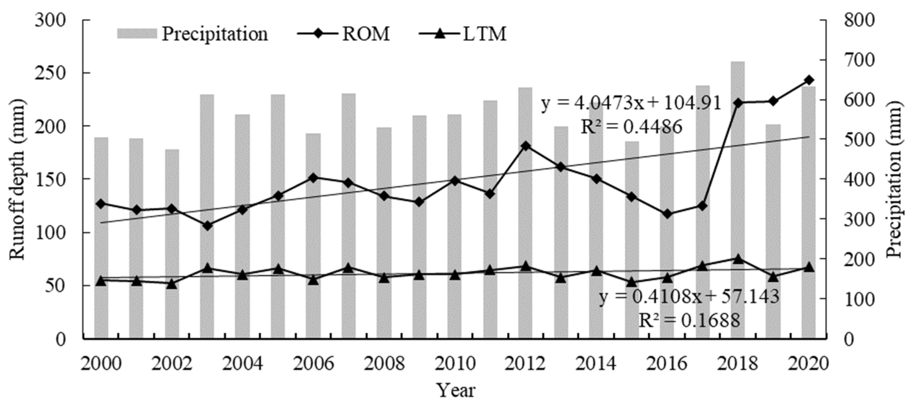
Over the period of 2000–2020, both the ROM and LTM methods showed an overall increase in runoff depth (Figure 5). The ROM results exhibited a more pronounced increase trend, with a significant 91% increase observed over 21 years. Notably, there was a substantial surge in runoff depth after 2017. Moreover, the ROM results indicated that changes in precipitation have a delayed and cumulative effect on runoff depth, such as during the years of 2003–2004 and 2012–2016. In contrast, the LTM results were relatively stable, with a 24% increase observed over 21 years (corresponding to a 23% increase in precipitation during the same period), and the variation in runoff depth was entirely controlled by precipitation.

3.1.3. Sub-Watershed Comparison

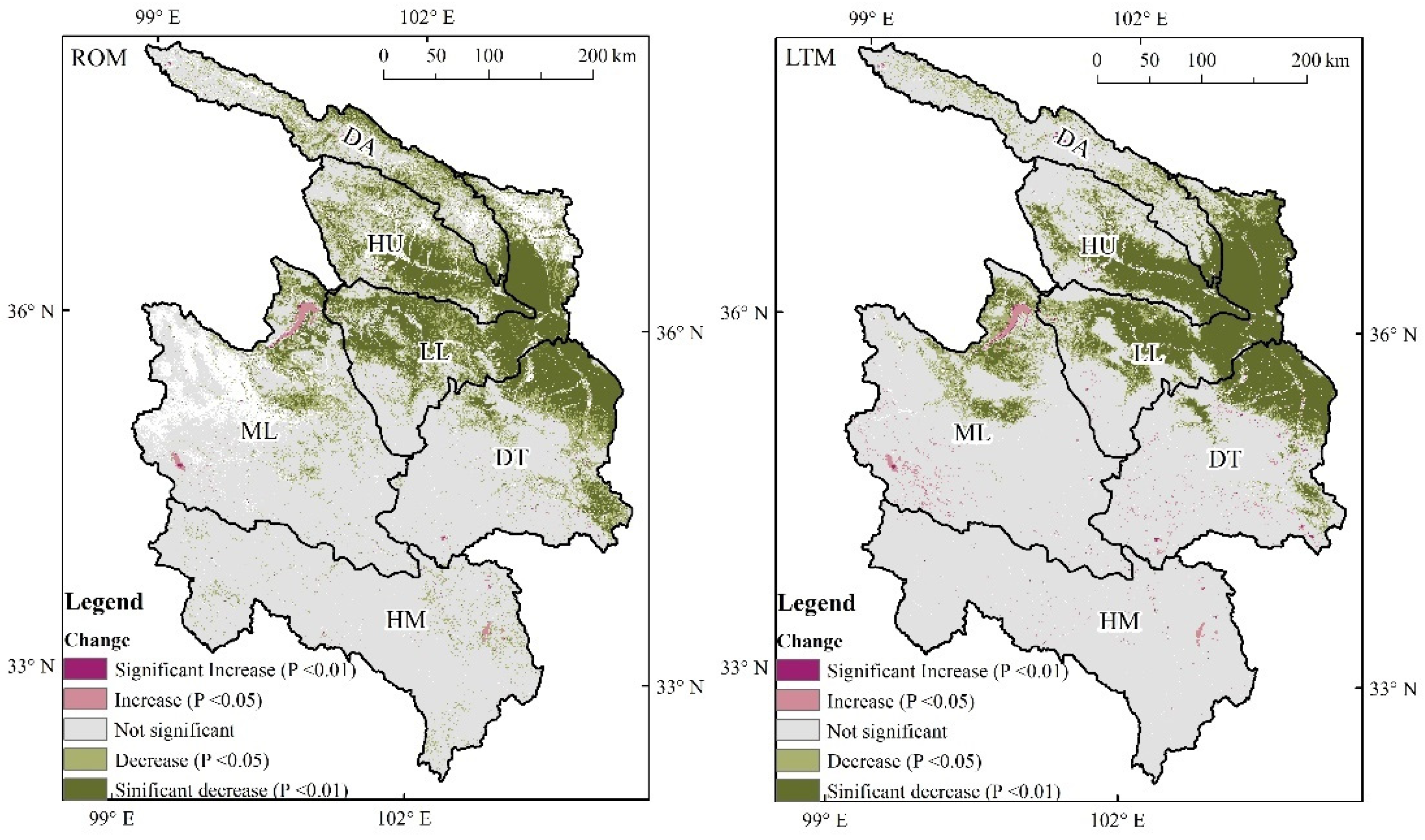
The finding revealed that the ROM method calculated a substantial increase (p < 0.01) in runoff depth in all sub-watersheds, while LTM results only showed an increase (p < 0.05) in specific regions, such as ML, DT, and HM, with no significant changes in other sub-watersheds (Figure 6). This is in agreement with the overall basin trend observed in Figure 5.
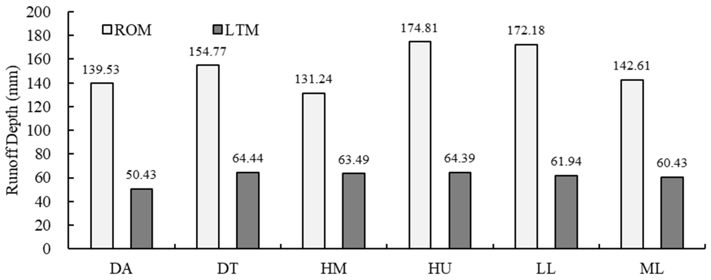
In comparison to the mean value of runoff depth across various sub-watersheds, the results obtained from ROM were considerably higher than those from LTM. The ROM outcomes reveal substantial differences among the different sub-watersheds. The sub-watershed HM had the lowest runoff depth, measuring 131.24 mm, and it mainly comprises alpine meadow and wetland ecosystems. Conversely, sub-watershed HU had the highest runoff depth, measuring 174.81 mm, and it is mainly characterized by farmland and urban construction land. In contrast, the LTM outcomes indicate that the variation between HM and HU is indistinct, and the maximum runoff depth is observed in DT (Figure 7).

3.2. Change in Water Conservation

3.2.1. Spatial Variation

The average water conservation from 2000 to 2020 was calculated by two methods (ROM and LTM), respectively (Figure 8). The results obtained from both methods exhibit a general pattern of high values in the south and low value in the north but show different spatial distribution patterns. Specifically, the areas with high values (>100 mm) in the ROM calculation results are predominantly concentrated in the southern HM sub-watershed. However, the LTM calculation results reveal that most areas in the basin possess a water conservation capacity exceeding 100 mm. Furthermore, the ROM result showed an average water conservation of 68.96 mm, while the LTM result was significantly higher, measuring 118.86 mm.

3.2.2. Time Variation

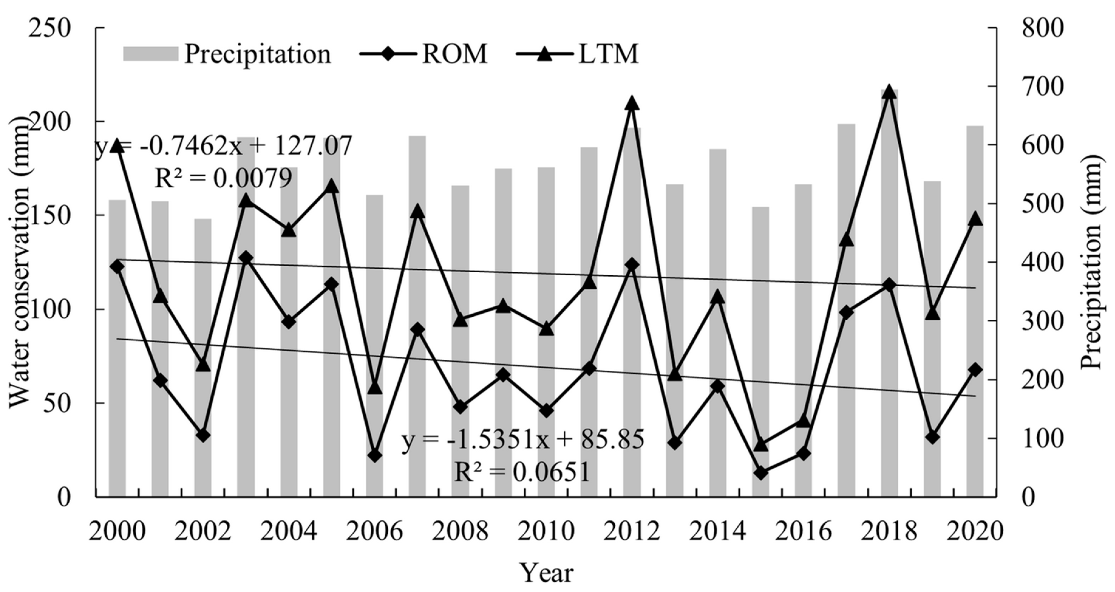
Over the period of 2000 to 2020, the water conservation amount calculated using two distinct methods (ROM and LTM) exhibited a gradual decline, as evidenced in Figure 9. Both methods show a similar trend of interannual variation, indicating that the water conservation capacity is particularly sensitive to changes in precipitation. Nonetheless, ROM is less influenced by precipitation when compared to LTM, mainly due to its interannual fluctuations features. The ROM result portrays a distinct pattern of decreasing water conservation capacity, indicating a decline of 45% over the 21-year period. In contrast, the results generated by LTM show greater stability with a decrease of 21% over the same period (the precipitation increased by 23% in the same period). Overall, the water conservation amount obtained through LTM tends to be overestimated when compared with the result obtained through ROM and exhibits more pronounced fluctuations.

3.2.3. Sub-Watershed Comparison

The spatial pattern of the water conservation trend calculated by the two methods is consistent. indicating a significant decrease (p < 0.01) in HU, LL, and DT in the northeast region, which is mainly characterized by farmland and construction land. However, there was no significant change observed in most other regions. The southern part of the basin, dominated by alpine grassland and wetland ecosystem, exhibits a relatively stable water conservation capacity (Figure 10).
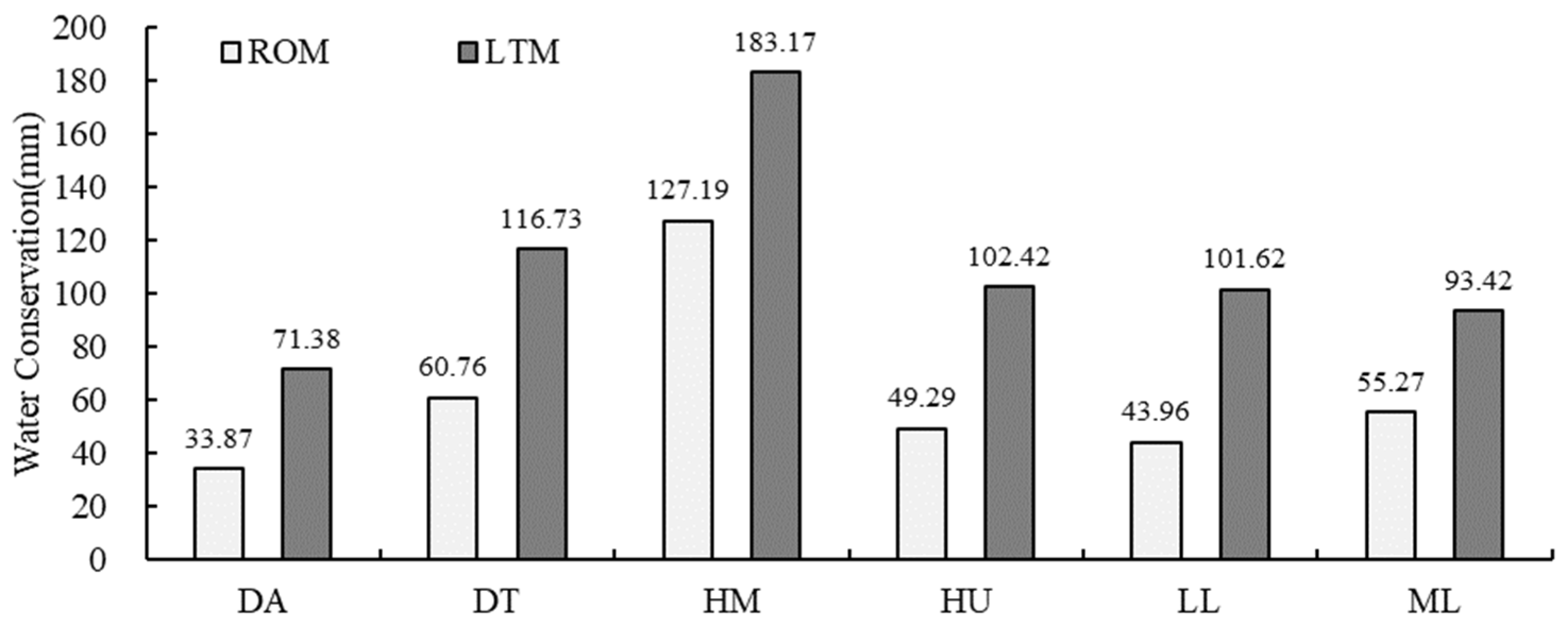
In comparison to the mean value of water conservation in various sub-watersheds, the water conservation capacity calculated by LTM was considerably greater than that obtained by ROM. Both methods reveal that the water conservation capacity of the DA sub-watershed is the lowest, while that of HM sub-watershed is the highest (as depicted in Figure 11). This trend is associated with the fact that the northern region of the entire basin receives relatively lower precipitation compared to the southern region, which receives comparatively higher precipitation.

3.3. Characteristics of Runoff Coefficient

3.3.1. Spatial Characteristics

When comparing the two methods, it was found that the ROM generated a higher runoff coefficient than the LTM (Figure 12). Moreover, areas covered by wetlands and natural vegetation exhibited a lower runoff coefficient of less than 20%, while farmland and bare land had a higher runoff coefficient of more than 30%. However, the LTM-based results masked the spatial heterogeneity of the runoff coefficient, with natural vegetation and water body having less than a 10% runoff coefficient and farmland having a runoff coefficient between 10% and 20%. Conversely, the spatial pattern of the runoff coefficient calculated by the ROM showed a higher value in the north and lower value in the south, which is more consistent with the spatial pattern of water conservation capacity.

3.3.2. Time Characteristics

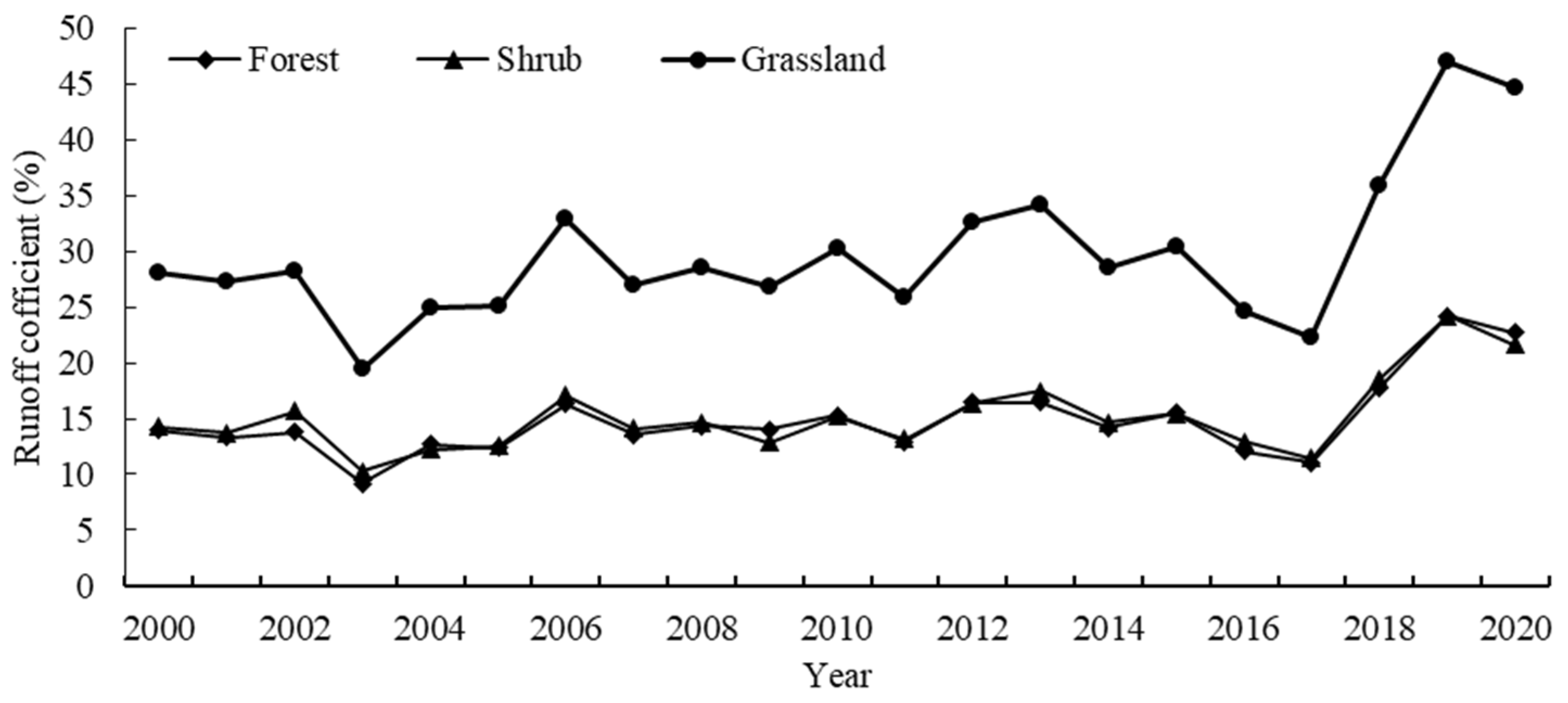
The use of LTM can only provide static values of runoff coefficient for different ecosystems, while ROM is capable of producing spatial distribution of the annual runoff coefficient. In this study, three types of ecosystems, namely forest, shrub, and grassland, were selected to analyze the annual change in the average value (Figure 13). The findings demonstrate that the runoff coefficient obtained by ROM is higher than the results of the runoff plot test, which reflects the overall characteristics of the landscape scale ecosystem. Furthermore, the grassland ecosystem shows significant fluctuations in the runoff coefficient, with variations of more than one time between different years (2003 and 2019), while forests and shrubs exhibit relatively stable trends.

3.3.3. Sub-Watershed Comparison

The analysis of the runoff coefficient of different ecosystem types in various sub-watersheds reveals significant spatial heterogeneity (Figure 14). Specifically, the forest runoff coefficient in DA and HM is 17.80% and 10.02%, respectively, while the grassland runoff coefficient in LL and HM is 35.96% and 24.83%, respectively.

4. Discussion

Accurate assessment of ecosystem status is a prerequisite for regional ecological protection management and decision making, particularly in regions with disparate natural resources endowment and unbalanced ecological functions, Doing so helps to identify and quantify spatiotemporal differences and changes in ecosystem quality and function. The quantification and spatiotemporal pattern analysis of regional water conservation capacity, an essential function of the natural ecosystem, are critical to achieving regional ecological protection and sustainable development. LTM relies mainly on data from runoff plots and small-scale eco-hydrological experiments to determine the runoff coefficients of different ecosystems and then employs precipitation data to estimate the spatiotemporal pattern of runoff depth and the water conservation capacity of ecosystems. Based on the comparative analysis, we have identified three main deficiencies of this approach:
The first deficiency of LTM is the absence of actual runoff data at the basin scale, which results in the estimation method being more akin to “simulation” than “assessment”. The assessment results are primarily driven by climate factors, such as precipitation. Secondly, the local scale rainfall experiment-observation-generated runoff coefficient has evident limitations in describing the runoff capacity of the landscape and regional scale ecosystem and will significantly underestimate the runoff capacity of the area dominated by vegetation distribution. This is primarily because the experimental design typically selects the “special” situation where the vegetation presents continuous distribution in space, and other geographical elements are almost entirely eliminated. Thirdly, as a fixed constant, the runoff coefficient is restricted not only in its ability to accurately describe the interannual change of the water conservation capacity of the ecosystem, but also in its ability to meet the requirements of regional ecological protection management decisions. Our findings underscore the importance of considering the spatial variability of the runoff coefficient in assessing water resource availability and management strategies in different sub-watersheds.
The presented ROM method serves as a viable alternative to the LTM approach for assessing the water conservation capacity of regional ecosystems. A key advantage of ROM lies in its ability to incorporate actual runoff data observed by hydrological stations, enabling quantitative allocation of this data to every pixel across the entire basin space. This process integrates differences in the underlying soil types’ runoff production capacity, in addition to referencing the differences in ecosystem types’ runoff production capacity. Thus, this new assessment method provides a more accurate and continuous characterization of spatiotemporal changes, allowing for the generation of spatiotemporal continuous runoff coefficient data sets that can facilitate more informed and scientific macro-ecosystem protection decisions. In comparison, LTM’s ecosystem-type-based runoff coefficient determination method not only disregards interannual variability in runoff coefficient values but also underestimates the surface runoff at a regional scale while overestimating the regional water conservation capacity, causing increased uncertainty in the overall planning and layout of regional ecological protection. Consequently, LTM may not be suited to support the coordinated development of ecological protection and economic development between the upstream and downstream areas of the basin.
Despite the strengths of the assessment method proposed in this study, several uncertainties remain. Firstly, due to the presence of concentrated farmland in the northeast of the basin and small cities, there is a risk of underestimating water consumption and then overestimating regional water conservation capacity. Secondly, the impact of terrain slope was not considered in the study design and therefore the runoff production capacity of the ecosystem at a smaller watershed or landscape scale. This is particularly important given that in the same ecosystem type and soil conditions, steep slopes tend to have more runoff than gentle slopes. Thirdly, the evaluation of the water conservation capacity of the ecosystem only considered the observation data of hydrological stations at the inlet and outlet of the basin, as there was insufficient data available for internal sub-watershed nodes. As a result, the study did not account for the scale effect on water conservation capacity. We believe that increasing the quantity of actual observation data is the most effective way to address these uncertainties in the evaluation methods and models.

5. Conclusions

Compared to the LTM method, the ROM method for estimating the spatial distribution of surface runoff offers practical advantages that maximize the integration of data observed by hydrological stations and provide a more accurate quantification and spatial pattern of the actual runoff of the basin runoff. Additionally, ROM inherits the accuracy of ecosystem-type data resolution, which may be obtained from high resolution satellite remote sensing, thus enabling a fine description of the spatial pattern of surface runoff. Furthermore, the ROM not only indicates the direct influence of precipitation on interannual variation in runoff depth but also highlights the characteristics of delay and accumulation in a year with a large fluctuation of rainfall. As such, ROM provides a more comprehensive reflection of the changes in the underlying surface and ecosystem in the basin.
The spatial distribution patterns and temporal variation characteristics of water conservation estimates generated using LTM and ROM exhibit similarities. The results indicate that farmland plays a significant role in reducing the regional water conservation capacity on a long-term scale. However, the LTM results may be subject to significant overestimation due to the lack of actual runoff observation data, particularly at the sub-watershed scale. Specifically, the overestimation of water conservation capacity is one to two times higher at the whole basin scale and, two to three times higher at the sub-watershed scale (such as DA, HU, LL, etc.).
The utilization of the time-space dynamic data set derived from ROM’s runoff coefficient is beneficial in comprehending the mechanism behind the runoff coefficient. Notably, the interannual variation patterns of the runoff coefficient should not be disregarded. Moreover, in comparable rainfall conditions, the same ecosystem type’s runoff coefficient could have significant discrepancies in different sub-watersheds (such as DA and HM), which highlights the ecosystem’s zonal geographical distribution attributes. As such, relying solely on the “ideal” runoff coefficient obtained from runoff plot experiments is inadequate to accurately assess water conservation in larger landscapes and regional scales. This insufficiency is also the primary cause of the substantial overestimation in ecosystem water conservation assessment by LTM.

Author Contributions

Conceptualization, P.H.; methodology, J.Z. and W.Z.; formal analysis, J.Z. and Y.C.; data curation, H.G., D.J., H.Z. and M.Y.; writing—original draft preparation, J.Z. All authors have read and agreed to the published version of the manuscript.

Funding

This research was funded by the National Key R & D Program of China (grant number. 2021YFF0703903) and Regular Remote Sensing Survey and Assessment of National Ecological Status of China (Grant No. 22110499001001).

Data Availability Statement

Not applicable.

Acknowledgments

The author is grateful for the suggestions provided by Yanda Xu (Natural Ecological Protection Department of the Ministry of Ecological Environment of the People’s Republic of China).

Conflicts of Interest

The authors declare no conflict of interest.

References

  1. Renard, K.G.; Foster, G.R.; Weesies, G.A. Predicting Soil Erosion by Water: A Guide to Conservation Planning with the Revised Universal Soil Loss Equation (RUSLE), 1st ed.; U.S. Department of Agriculture, Agricultural Research Service: Washington, DC, USA, 1997; Volume 404. [Google Scholar]
  2. Fryrear, D.W.; Bilbro, J.D.; Saleh, A.; Schomberg, H.; Stout, J.E.; Zobeck, T.M. RWEQ: Improved wind erosion technology. J. Soil Water Conserv. 2000, 55, 183–189. [Google Scholar]
  3. Lu, Y.; Hu, J.; Sun, F.; Zhang, L.W. Water retention and hydrological regulation: Harmony but not the same in terrestrial hydrological ecosystem services. Acta Ecol. Sin. 2015, 35, 5191–5196. [Google Scholar]
  4. Xi, Q.J.; Zhong, H.; Wang, T.; He, T.; Gao, H.; Xia, J.; Wang-Erlandsson, L.; Tang, Q.; Liu, J. Spatio-temporal variation of gray-green-blue storage capacity in nine major basins of China. Chin. Sci. Bull.-Chin. 2021, 66, 4437–4448. [Google Scholar] [CrossRef]
  5. Wang, Y.F.; Ye, A.Z.; Qiao, F.; Li, Z.S.; Miu, C.Y.; Di, Z.H.; Gong, W. Review on connotation and estimation method of water conservation. South-North Water Transf. Water Sci. Technol. 2021, 19, 1041–1071. [Google Scholar]
  6. Gao, H.K.; Liu, J.G.; Gao, G.Y. Ecological and hydrological perspectives of the water retention concept. Acta Geogr. Sin. 2023, 78, 139–148. [Google Scholar]
  7. Sun, G.; Zhang, L.; Wang, Y.H. On accurately defining and quantifying the water retention services of forests. Acta Ecol. Sin. 2023, 43, 9–25. [Google Scholar]
  8. Wei, P.R.; Chen, S.Y.; Wu, M.H.; Deng, Y.F.; Xu, H.J.; Jia, Y.L.; Liu, F. Using the InVEST Model to Assess the Impacts of Climate and Land Use Changes on Water Yield in the Upstream Regions of the Shule River Basin. Water 2021, 13, 1250. [Google Scholar] [CrossRef]
  9. Daneshi, A.; Brouwer, R.; Najafinejad, A.; Panahi, M.; Zarandian, A.; Maghsood, F.F. Modeling the impacts of climate and land use change on water security in a semi-arid forested watershed using InVEST. J. Hydrol. 2021, 593, 18. [Google Scholar] [CrossRef]
  10. Lu, W.; Xia, W.; Shoemaker, C.A. Surrogate Global Optimization for Identifying Cost-Effective Green Infrastructure for Urban Flood Control with a Computationally Expensive Inundation Model. Water Resour. Res. 2022, 58, 23. [Google Scholar] [CrossRef]
  11. Zheng, H.; Li, Y.F.; Robinson, B.E.; Liu, G.; Ma, D.C.; Wang, F.C.; Lu, F.; Ouyang, Z.Y.; Daily, G.C. Using ecosystem service trade-offs to inform water conservation policies and management practices. Front. Ecol. Environ. 2016, 14, 527–532. [Google Scholar] [CrossRef]
  12. Ouyang, Z.Y.; Zheng, H.; Xiao, Y.; Polasky, S.; Liu, J.G.; Xu, W.H.; Wang, Q.; Zhang, L.; Xiao, Y.; Rao, E.M.; et al. Improvements in ecosystem services from investments in natural capital. Science 2016, 352, 1455–1459. [Google Scholar] [CrossRef]
  13. Gong, S.; Xiao, Y.; Zheng, H.; Xiao, Y.; Ouyang, Z.Y. Spatial patterns of ecosystem water conservation in China and its impact factors analysis. Acta Ecol. Sin. 2017, 37, 2455–2462. [Google Scholar]
  14. Wu, X.; Shi, W.J.; Tao, F.L. Estimations of forest water retention across China from an observation site-scale to a national-scale. Ecol. Indic. 2021, 132, 10. [Google Scholar] [CrossRef]
  15. Zhang, B.; Wang, S.; Li, Q.; Xie, G.D. Spatio-temporal changes of water conservation service in the Beijing-Tianjin sandstorm source control project area. Acta Ecol. Sin. 2021, 41, 7530–7541. [Google Scholar]
  16. Reid, W.V.; Mooney, H.A.; Cropper, A.; Capistrano, D.; Chopra, K. Ecosystems and Human Well-Being—Synthesis: A Report of the Millennium Ecosystem Assessment, 1st ed.; Island Press: Washington, DC, USA, 2005. [Google Scholar]
  17. Agudelo, C.A.R.; Bustos, S.L.H.; Moreno, C.A.P. Modeling interactions among multiple ecosystem services. A critical review—ScienceDirect. Ecol. Model. 2020, 429, 22. [Google Scholar] [CrossRef]
  18. Hasan, S.S.; Zhen, L.; Miah, M.G.; Ahamed, T.; Samie, A. Impact of land use change on ecosystem services: A review. Environ. Dev. 2020, 34, 100527. [Google Scholar] [CrossRef]
  19. GB/T 38582-2020; Specification for Evaluation of Forest Ecosystem Service Function. National Forestry and Grassland Administration: Beijing, China, 2020. Available online: http://www.forestry.gov.cn/chinagreen/49/20210903/151956149968742.html (accessed on 2 March 2020).
  20. HJ 1173-2021; Technical Specifications for Investigation and Assessment of National Ecological Status—Ecosystem Service Assessment. Ministry of Ecology and Environment, PRC: Beijing, China, 2021. Available online: https://www.mee.gov.cn/ywgz/fgbz/bz/bzwb/stzl/202106/t20210615_839011.shtml (accessed on 6 August 2021).
  21. Wang, Q.; Ouyang, Z.Y. Eeo-Environment Investigation and Assessment from 2000 to 2010 with Remote Sensing of China, 1st ed.; Science Press: Beijing, China, 2014. [Google Scholar]
  22. Guidelines for Evaluating the Carrying Capacity of Resources and Environment and the Suitability of Land and Space Development (for Trial). Available online: http://www.gov.cn/zhengce/zhengceku/2020-01/22/content_5471523.htm (accessed on 19 January 2020).
  23. Technical Guide for Delimitation of Ecological Protection Red Line. Available online: https://www.mee.gov.cn/gkml/hbb/bwj/201505/t20150518_301834.htm (accessed on 8 May 2015).
  24. Gao, J.X.; Zou, C.X.; Zhang, K.; Xu, M.J.; Wang, Y. The establishment of Chinese ecological conservation redline and insights into improving international protected areas. J. Environ. Manag. 2020, 264, 110505. [Google Scholar] [CrossRef]
  25. Bedient, P.; Huber, W.; Vieux, B. Hydrology and Floodplain Analysis, 6th ed.; Pearson Publishing: Boston, MA, USA, 2013. [Google Scholar]
  26. Birkinshaw, S.J.; O’Donnell, G.; Glenis, V.; Kilsby, C. Improved hydrological modeling of urban catchments using runoff coefficients. J. Hydrol. 2021, 594, 125884. [Google Scholar] [CrossRef]
  27. Yin, H.L.; Zhao, Z.C.; Wang, R.Q.; Xu, Z.X.; Li, H.Z. Determination of urban runoff coefficient using time series inverse modeling. J. Hydrodyn. 2017, 29, 898–901. [Google Scholar] [CrossRef]
  28. Sajjad, R.U.; Kim, K.J.; Memon, S.; Sukhbaatar, C.; Paule, M.C.; Lee, B.Y.; Lee, C.H. Characterization of Stormwater Runoff from a Light Rail Transit Area. Water Environ. Res. 2015, 87, 813–822. [Google Scholar] [CrossRef] [PubMed]
  29. Maetens, W.; Poesen, J.; Vanmaercke, M. How effective are soil conservation techniques in reducing plot runoff and soil loss in Europe and the Mediterranean? Earth-Sci. Rev. 2012, 115, 21–36. [Google Scholar] [CrossRef]
  30. Sadeghi, S.H.R.; Gholami, L.; Sharifi, E.; Darvishan, A.K.; Homaee, M. Scale effect on runoff and soil loss control using rice straw mulch under laboratory conditions. Solid Earth 2015, 6, 1–8. [Google Scholar] [CrossRef]
  31. Fang, N.F.; Shi, Z.H.; Li, L.; Guo, Z.L.; Liu, Q.J.; Ai, L. The effects of rainfall regimes and land use changes on runoff and soil loss in a small mountainous watershed. Catena 2012, 99, 1–8. [Google Scholar] [CrossRef]
  32. Merten, G.H.; Araujo, A.G.; Biscaia, R.C.M.; Biscaia, R.C.M.; Barbosa, G.M.C.; Conte, O. No-till surface runoff and soil losses in southern Brazil. Soil Tillage Res. 2015, 152, 85–93. [Google Scholar] [CrossRef]
  33. Zheng, H.Y.; Miao, C.Y.; Zhang, G.H.; Li, X.Y.; Wang, S.; Wu, J.W.; Gou, J.J. Is the runoff coefficient increasing or decreasing after ecological restoration on China’s Loess Plateau? Int. Soil Water Conserv. Res. 2021, 9, 333–343. [Google Scholar] [CrossRef]
  34. Zeng, Z.Y.; Tang, G.Q.; Hong, Y.; Zeng, C.; Yang, Y. Development of an NRCS curve number global dataset using the latest geospatial remote sensing data for worldwide hydrologic applications. Remote Sens. Lett. 2017, 8, 528–536. [Google Scholar] [CrossRef]
  35. Xiong, J.H.; Yin, J.B.; Guo, S.L.; He, S.K.; Chen, J.; Abhishek. Annual runoff coefficient variation in a changing environment: A global perspective. Environ. Res. Lett. 2022, 17, 12. [Google Scholar] [CrossRef]
  36. Veerkamp, C.J.; Loreti, M.; Benavidez, R.; Jackson, B.; Schipper, A.M. Comparing three spatial modeling tools for assessing urban ecosystem services. Ecosyst. Serv. 2023, 59, 12. [Google Scholar] [CrossRef]
  37. Machado, R.E.; Cardoso, T.O.; Mortene, M.H. Determination of runoff coefficient (C) in catchments based on analysis of precipitation and flow events. Int. Soil Water Conserv. Res. 2022, 10, 208–216. [Google Scholar] [CrossRef]
  38. Shen, Y.P. National 1:250,000 Three-Level River Basin Data Set. Available online: www.ncdc.ac.cn (accessed on 23 January 2019).
  39. HJ 1166-2021; Technical Specifications for Investigation and Assessment of National Ecological Status—Remote Sensing Interpretation and Field Verification of Ecosystem. Ministry of Ecology and Environment, PRC: Beijing, China, 2021. Available online: https://www.mee.gov.cn/ywgz/fgbz/bz/bzwb/stzl/202106/t20210615_838997.shtml (accessed on 6 August 2021).
  40. Liu, J.Y.; Kuang, W.H.; Zhang, Z.X.; Xu, X.L.; Qin, Y.W.; Ning, J.; Zhou, W.C.; Zhang, S.W.; Li, R.D.; Yan, C.Z.; et al. Spatiotemporal characteristics, patterns, and causes of land-use changes in China since the late 1980s. J. Geogr. Sci. 2014, 24, 195–210. [Google Scholar] [CrossRef]
  41. Chu, X.Y.; Wang, Y.J.; Wang, Y.Q.; Cheng, C.; Xia, Y.P.; Wu, Y.; Chen, L. Runoff generation characteristics on three time scales for typical stands in Jinyun Mountain, Chongqing City. J. Beijing For. Univ. 2008, 30, 103–108. [Google Scholar]
  42. Kong, W.J.; Zhou, B.Z.; Fu, M.Y.; Li, Z.C.; Xie, J.Z.; Wu, M. Effects of different land-use on characteristics of soil and water conservation. J. Nanjing For. Univ. (Nat. Sci. Ed.) 2009, 33, 57–61. [Google Scholar]
  43. Wang, X.D.; Zhang, H.J.; Cheng, J.H.; Sun, Y.H. Characteristics of Runoff on Forest Vegetation Slopes in Three Gorges Area. Res. Soil Water Conserv. 2008, 15, 1–3. [Google Scholar]
  44. Chen, B.; Wang, M.; Yao, H.E.; Hou, J.J.; Mao, Y.Q. Analysis of monitoring results of water and soil conservation monitoring points in the runoff area of Tangyu River basin from 2017 to 2019. Soil Water Conserv. China 2021, 5, 55–57. [Google Scholar]
  45. Feng, W.F.; Wang, Z.Q.; Shan, Y.X.; Li, Y.F.; Du, W.Z. Study on Variation of Runoff of Typical Forestland in Southern Mountain of Henan Province. J. Henan For. Sci. Technol. 2009, 29, 16–20. [Google Scholar]
  46. Zhu, Y.Q.; Zhao, Z.B.; Qi, G.P. Effects of Vegetation Types and Rainfall Regimes on Slope Erosion and Sediment Yield in Loess Hilly and Gully Region. J. Soil Water Conserv. 2019, 33, 9–16. [Google Scholar]
  47. Dong, H.B.; Zhang, J.J.; Zhang, B.; Zhang, R.; Zhou, X.X. Research on Rain-runoff Relationship in Different Land Use Types on the Loess Area in Western Shanxi Province. J. Arid Land Resour. Environ. 2009, 23, 110–116. [Google Scholar]
  48. Duan, W.B.; Liu, S.C. Analysis on Runoff and Sediment Yields of Water Conservation Forests in Lianhua Lake Reservoir Area. J. Soil Water Conserv. 2006, 20, 12–15. [Google Scholar]
  49. Song, J.H. Study on Forest Hydrological and Ecological Functions of Jinyun Mountain in Chongqing. Ph.D. Thesis, Beijing Forestry University, Beijing, China, 2008. [Google Scholar]
  50. Li, J.Y.; Miao, X.X.; Wang, Y.X.; Yu, D.M.; Zhang, X.Y.; Hu, X.S.; Xu, T.; Shen, Z.Y.; Liu, C.Y.; Yan, C.; et al. The Characteristics of Runoff and Sediment Yield on Slope Surface under Different Herbs and Slope Shapes in Loess Regions of Xining Basin. J. Salt Lake Res. 2022, 30, 33–45. [Google Scholar]
  51. Wei, X.P.; Xie, S.Y.; Zhang, Z.W.; Chen, Z.X. Characteristics of surface soil erosion of karst valley in different land use types at Nanping in Chongqing. Trans. Chin. Soc. Agric. Eng. 2011, 27, 42–46. [Google Scholar]
  52. Li, M.; Song, X.Y.; Shen, B.; Li, H.Y.; Meng, C.X. Influence of vegetation change on producing runoff and sediment in gully region of Loess Plateau. J. Northwest Sci-Tech Univ. AgricuUAure For. (Nat. Sci. Ed.) 2006, 34, 117–120. [Google Scholar]
  53. Zhang, Y.F.; Wang, X.P.; Hu, R.; Pan, Y.X.; Raradeloc, M. Rainfall partitioning into throughfall, stemflow and interception loss by two xerophytic shrubs within a rain-fed re-vegetated desert ecosystem, northwestern China. J. Hydrol. 2015, 527, 1084–1095. [Google Scholar] [CrossRef]
  54. Liu, Y.J.; Yang, J.; Hu, J.M.; Tang, C.J.; Zheng, H.J. Characteristics of the surface—Subsurface flow generation and sediment yield to the rainfall regime and land-cover by long-term in-situ observation in the red soil region, Southern China. J. Hydrol. 2016, 539, 457–467. [Google Scholar] [CrossRef]
  55. Annual Hydrological Report of P.R. China. Hydrological Data of Yellow River Basin; Hydrology Department of the Ministry of Water Resources of the People’s Republic of China Press: Beijing, China, 2001–2021.
  56. Mu, Q.Z.; Zhao, M.S.; Running, S.W. MODIS Global Terrestrial Evapotranspiration (ET) Product (NASA MOD16A2/A3) Collection 5. NASA Headquarters. Numerical Terradynamic Simulation Group Publications. 268. 2013. Available online: https://scholarworks.umt.edu/ntsg_pubs/268 (accessed on 8 November 2019).
  57. Kendall, M.G. Rank Correlation Methods, 1st ed.; Oxford University Press: Oxford, UK, 1948. [Google Scholar]
  58. Mann, H.B. Non-parametric tests against trend. Econometrica 1945, 13, 245–259. [Google Scholar] [CrossRef]
  59. Sen, P.K. Estimates of the Regression Coefficient Based on Kendall’s Tau. J. Am. Stat. Assoc. 1968, 63, 1379–1389. [Google Scholar] [CrossRef]
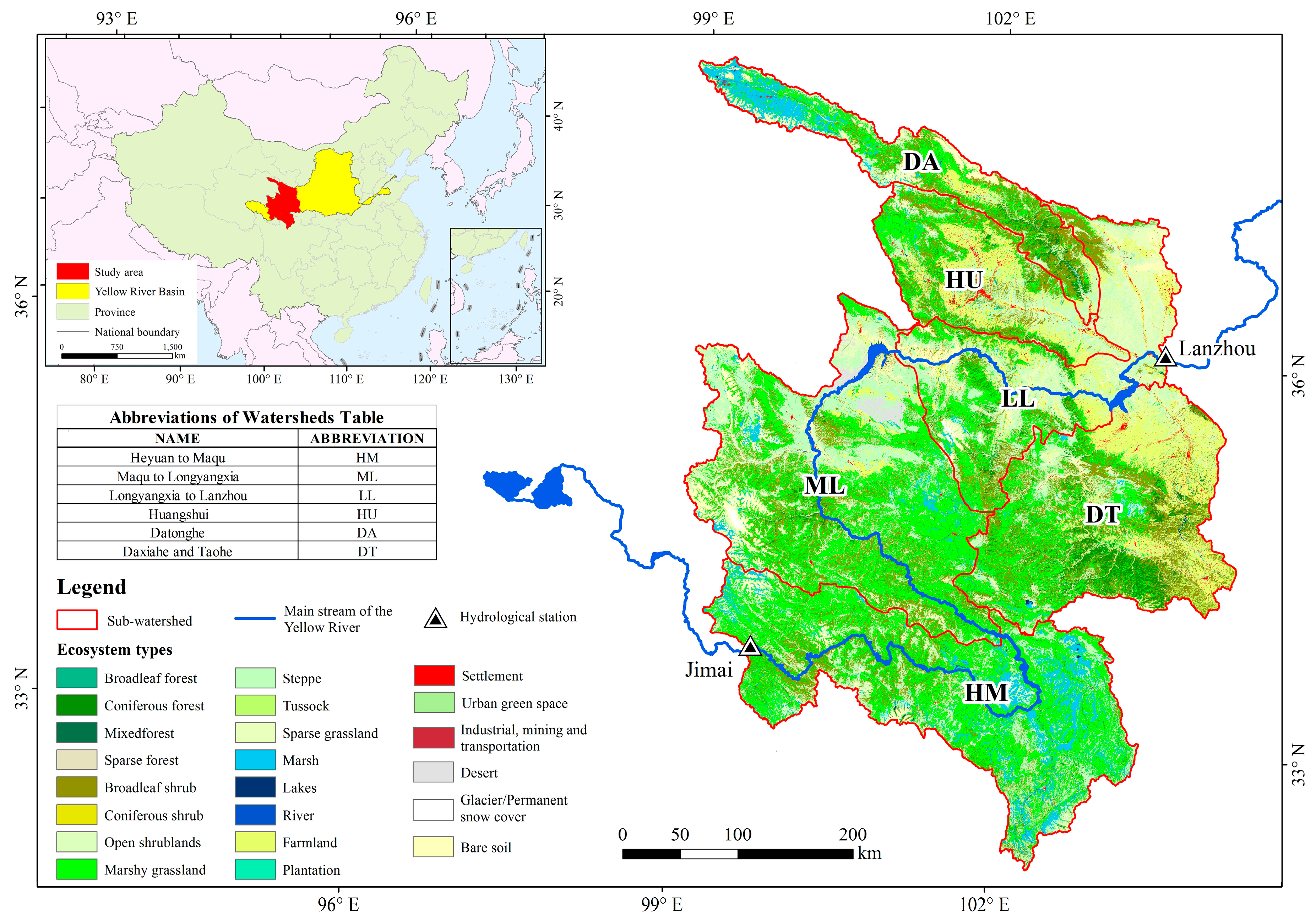
Figure 1. Spatial distribution of the ecosystem in the study area.
Water 15 01475 g001
Figure 2. Technical flowchart.
Water 15 01475 g002
Figure 3. Schematic diagram of the logic principle.
Water 15 01475 g003
Figure 4. Spatial distribution of runoff depth calculated by two methods.
Water 15 01475 g004
Figure 5. Interannual variation in runoff depth and precipitation.
Water 15 01475 g005
Figure 6. Spatial distribution of runoff depth change calculated by two methods.
Water 15 01475 g006
Figure 7. Comparison of average runoff depth in different sub-watersheds.
Water 15 01475 g007
Figure 8. Spatial distribution of water conservation calculated by two methods.
Water 15 01475 g008
Figure 9. Interannual variation in water conservation and precipitation.
Water 15 01475 g009
Figure 10. Spatial distribution of water conservation change calculated by two methods.
Water 15 01475 g010
Figure 11. Comparison of average water conservation in different sub-watersheds.
Water 15 01475 g011
Figure 12. Spatial distribution of runoff coefficient calculated by two methods.
Water 15 01475 g012
Figure 13. Interannual variation in runoff coefficient of forest, shrub and grassland.
Water 15 01475 g013
Figure 14. The runoff coefficient of different ecosystem types in sub-watersheds.
Water 15 01475 g014
Table 1. Runoff coefficient (Rc) and runoff index of type (Rit).
Ecosystem TypesLiteratureRc (%)Rit
Broadleaf forest[41,42,43,44,45]3.331.55
Coniferous forest[13,42,46,47,48]2.151.00
Mixed forest[45,49]2.41.12
Sparse forest[47,50]16.027.45
Broadleaf shrub[41,46]3.581.67
Coniferous shrub[46]3.411.59
Open shrublands[47,50]16.027.45
Marshy grassland[48]9.114.24
Steppe[44,46,50]12.345.74
Tussock[47,51]10.184.73
Sparse grassland[47,50]16.027.45
Marsh *-00
Lakes *-00
River *-00
Farmland[52]49.6923.11
Plantation[41,42,43,44,45,46,47,48,49,50]4.622.15
Settlement[26]9041.86
Urban green space[41,42,43,44,45,46,47,48,49,50,51,52]7.913.68
Industrial, mining and transportation[26]73.3334.11
Desert *[53]3013.95
Glacier/Permanent snow cover-00
Bare soil[54]2511.63
Note: * This study assumes that the runoff coefficient of marsh, lakes, river, and glacier/permanent snow cover is 0.
Table 2. CN * of different HSG and runoff index of soil (Ris).
Ecosystem TypesCNACNBCNCCNDRis (A)Ris (B)Ris (C)Ris (D)
Broadleaf forest366275811.001.722.082.25
Coniferous forest376275811.001.682.032.19
Mixed forest386275811.001.631.972.13
Sparse forest728283871.001.141.151.21
Broadleaf shrub456575801.001.441.671.78
Coniferous shrub496979841.001.411.611.71
Open shrublands728283871.001.141.151.21
Marshy grassland496979841.001.411.611.71
Steppe496979841.001.411.611.71
Tussock496979841.001.411.611.71
Sparse grassland728283871.001.141.151.21
Marsh00000000
Lakes00000000
River00000000
Farmland677885891.001.161.271.33
Plantation526979841.001.331.521.62
Settlement808590951.001.061.131.19
Urban green space527079841.001.351.521.62
Industrial, mining, and transportation808590951.001.061.131.19
Desert728283871.001.141.151.21
Glacier/permanent snow cover00000000
Bare soil728283871.001.141.151.21
Note: * The values in Table 2 of the literature [34] are classified according to the ecosystem types in this table.
Disclaimer/Publisher’s Note: The statements, opinions and data contained in all publications are solely those of the individual author(s) and contributor(s) and not of MDPI and/or the editor(s). MDPI and/or the editor(s) disclaim responsibility for any injury to people or property resulting from any ideas, methods, instructions or products referred to in the content.