Article

Streamflow Simulation with High-Resolution WRF Input Variables Based on the CNN-LSTM Hybrid Model and Gamma Test

1
State Key Laboratory of Simulation and Regulation of Water Cycle in River Basin, China Institute of Water Resources and Hydropower Research, Beijing 100038, China
2
Beijing Water Conservation and Utilization Management Affairs Centre, Beijing 100142, China
*
Author to whom correspondence should be addressed.
Water 2023, 15(7), 1422; https://doi.org/10.3390/w15071422
Submission received: 13 March 2023 / Revised: 24 March 2023 / Accepted: 4 April 2023 / Published: 6 April 2023

Abstract

:
Streamflow modelling is one of the most important elements for the management of water resources and flood control in the context of future climate change. With the advancement of numerical weather prediction and modern detection technologies, more and more high-resolution hydro-meteorological data can be obtained, while traditional physical hydrological models cannot make full use of them. In this study, a hybrid deep learning approach is proposed for the simulation of daily streamflow in two mountainous catchments of the Daqing River Basin, northern China. Two-dimensional high-resolution (1 km) output data from a WRF model were used as the model input, a convolutional neural network (CNN) model was used to extract the physical and meteorological characteristics of the catchment at a certain time, and the long short-term memory (LSTM) model was applied to simulate the streamflow using the time-series data extracted by the CNN model. To reduce model input noise and avoid overfitting, the Gamma test method was adopted and the correlations between the input variables were checked to select the optimal combination of input variables. The performance of the CNN-LSTM models was acceptable without using the Gamma test (i.e., with all WRF input variables included), with NSE and RMSE values of 0.9298 and 9.0047 m3/s, respectively, in the Fuping catchment, and 0.8330 and 1.1806 m3/s, respectively, in the Zijingguan catchment. However, it was found that the performance of the model could be significantly improved by the use of the Gamma test. Using the best combination of input variables selected by the Gamma test, the NSE of the Fuping catchment increased to 0.9618 and the RMSE decreased to 6.6366 m3/s, and the NSE of the Zijingguan catchment increased to 0.9515 and the RMSE decreased to 0.6366 m3/s. These results demonstrate the feasibility of the CNN-LSTM approach for flood streamflow simulation using WRF-downscaled high-resolution data. By using this approach to assess the potential impacts of climate change on streamflow with the abundant high-resolution meteorological data generated by different climate scenarios, water managers can develop more effective strategies for managing water resources and reducing the risks associated with droughts and floods.

1. Introduction

Streamflow simulation and prediction in ungauged basins has always been a key area of hydrological research [1], and streamflow modelling is crucial for the management of water resources and flood control [2]. Streamflow modelling generally uses meteorological variables as forcing data to simulate the response of the watershed. The rainfall–runoff transformation process is highly nonlinear and is determined not only by external meteorological factors but also by the physical state of the catchment [3].
The Weather Research and Forecasting (WRF) model, an advanced mesoscale numerical weather prediction system, was collaboratively developed by several institutes including the National Center for Atmospheric Research (NCAR) and the National Centers for Environmental Prediction (NCEP) [4]. The WRF model can improve the spatial and temporal resolution of global prediction products and achieve refined and quantitative predictions of rainfall and other meteorological variables. A combination of the WRF-downscaled predictions and hydrological models can therefore provide an important method for streamflow modelling in ungauged or data-limited catchments. Bass et al. [5] used a regional climate model’s reanalysis-derived meteorological data as forcing data, simulated the realistic streamflow using WRF and a land surface model, and used a mathematical approach called the donor-basin method to regionalize parameters in ungauged basins. Tyson et al. [6] successfully simulated the streamflow response to snowmelt using a WRF–UEB hybrid model in the canyon portion of the Logan River watershed. Naabil et al. [7] used the WRF/WRF-Hydro coupling model to simulate the streamflow of the Tono Basin in Ghana from 1999 to 2013 and achieved a satisfactory performance, with a Nash–Sutcliff efficiency (NSE) coefficient of 0.78 and a Pearson’s correlation of 0.89. Wang et al. [8] coupled the WRF model with the Xinanjiang (XAJ) model to simulate the daily streamflow of the Shiquan catchment in the upper Han River basin, and comparison of the results of the uncoupled XAJ, random forest (RF), and XAJ–RF models showed that the best performance statistics were obtained from the XAJ–WRF model (NSE = 0.951, R = 0.978). Gu et al. [9] proposed an atmospheric–hydrological modeling system based on the WRF model and the Storm Water Management Model (SWMM) to simulate urban storm and flood events. For two heavy rainfall events in the study area, the model performed well, with the NSE values reaching 0.884 and 0.796, respectively.
Data-driven models represent an alternative to hydrological models and have been proven to be capable of using data to directly learn the relationship between streamflow and meteorological variables [10]. In recent years, with the development of computing power and improvements in data diversity, a new data-driven model, the deep learning long short-term memory (LSTM) model, has been developed and widely used. As a deep learning model, LSTM networks are designed to work with sequential data, which is a characteristic of hydrological time-series data. LSTM networks can effectively capture the temporal dependencies and patterns in the data, which can be useful for predicting future values [11,12,13]. Several studies have shown that LSTM models generally outperform traditional hydrological models. Xiang et al. [14] proposed an LSTM-based hourly flow prediction model for Clear Creek and the Upper Wapsipinicon River, and the results showed that the LSTM-based model outperformed linear regression, lasso regression, ridge regression, support vector regression (SVR), and Gaussian process regression (GPR) for all the stations in these two catchments. Thapa et al. [15] developed models based on the LSTM, nonlinear autoregressive exogenous (NARX), GPR, and SVR models for snowmelt-driven discharge modeling in a Himalayan basin, and the LSTM model achieved the best results followed by NARX, GPR, and SVR.
In spite of its many advantages, the LSTM model requires one-dimensional input data and cannot process high-resolution two-dimensional (gridded) meteorological data across the catchment. The convolutional neural network (CNN), another deep learning model, has a strong ability to capture the characteristics of spatial data [16,17] and has therefore been widely used in the image classification, edge detection, and face recognition fields in recent years [18,19,20]. Van et al. [21] used the CNN model to build a rainfall runoff model and compared it with traditional models such as artificial neural networks (ANN), genetic algorithm-simulated annealing (GA-SA), seasonal autoregressive integrated moving average (SARIMA), and autoregressive integrated moving average (ARIMA) in the simulation of streamflow at the Chau Doc and Can Tho stations in the Vietnamese Mekong Delta. The results showed that the CNN model outperformed the other models. Wang et al. [22] used CNN and SVM to assess the flood susceptibility of Shangyou County in China, and the results demonstrated that the CNN model produced more reliable and practical flood susceptibility maps. In addition, by constructing a CNN model based on SVM, it was possible to improve the prediction capability of SVM by 0.021–0.051 in terms of the area under the curve (AUC). Using a CNN, the two-dimensional hydrometeorological input data of a catchment can be converted into one-dimensional feature vectors, thus resolving the dimensionality problem related to the LSTM model input data. Barzegar et al. [23] compared the performance of the water level prediction by using CNN-LSTM, SVR, and RF models for Lake Michigan and Lake Ontario. It was found that the CNN-LSTM model outperformed the SVR and RF models at any given time. Li et al. [24] proposed a CNN-LSTM model based on rainfall radar maps to compute the runoff in Elbe River basin in Sachsen, and this CNN-LSTM model achieved good results in streamflow prediction for high-water periods (KGE = 0.75, NSE = 0.78) and low-water periods (KGE = 0.76, NSE = 0.81). Tran et al. [25] used PredCNN, a CNN-LSTM based emulator, to simulate the streamflow, water table depth, and total water storage of Taylor River basin and Little Washita basin, and the results were found to be consistent with the hydrological model ParFlow.
Overfitting is a common problem in deep learning models, leading to performances that are outstanding in training samples but unsatisfactory in test datasets. In the case of sufficient data, i.e., a sufficient number of data points, the main reason for overfitting is the noise of the input data. The Gamma test is regarded as an effective way to reduce noise through estimation of the best mean square error of the smoothing model for a given input [26], and can therefore help to identify the input data combination with the least noise. Malik et al. [27], Hassan and Hassan [28], and Panahi et al. [29] successfully used the Gamma test to select the best input combination before comparing the flow simulation performance of different hydrological models. Zhuo and Han [30] established a new soil moisture product directly applicable to hydrological modeling from multiple data sources, used the Gamma test to pre-evaluate selected data inputs, and found the best combination for data fusion; the new product had a significantly higher NSE of nearly 50% compared to the two most popular Soil Moisture products. Tian et al. [31] verified that the Gamma test can not only solve the problem of selecting the best input combination for data-driven models, but can also help identify the relative importance of input variables.
In this study, a CNN-LSTM hybrid model using WRF downscaling data was proposed for streamflow simulation, in which the CNN model was used to extract the physical and meteorological characteristics of the catchment at a certain time, and the LSTM model was applied to simulate the streamflow using the time-series data extracted by the CNN model. Prior to model construction, the Gamma test was used to identify appropriate combinations of variables from the high-resolution WRF meteorological outputs. Finally, the various combinations determined with the help of the Gamma test as well as an unscreened combination were each used as inputs for streamflow simulation, and the Nash–Sutcliffe efficiency coefficient (NSE) and root mean square error (RMSE) were used as criteria to analyze the performance of the model. The study was conducted on two mountainous catchments in the upstream area of the Daqing River Basin, North China. Using this approach under different climate scenarios can help water resource managers and flood control authorities to better prepare for future climate change impacts.

2. Study Area

Two mountainous catchments in the Daqing River Basin were selected as the study area, namely, the Fuping catchment in the south branch and the Zijingguan catchment in the north branch (Figure 1). The Daqing River Basin is located in North China, which has a typical semi-arid, semi-humid, warm continental monsoon climate. The Fuping and Zijingguan catchments cover areas of 2210 and 1760 km2, respectively. The elevation decreases from northwest to southeast with great variation, which produces a short flood confluence time. Coupled with high-intensity and short-duration precipitation, this has the potential to cause severe flood disasters. Most rainstorm events occur in the flood season (from June to September). There are 8 and 11 gauges located in the Fuping and Zijingguan catchments, respectively, and the streamflow is measured at the catchment outlets (Figure 1). These two catchments can represent the underlying surface characteristics of the small catchments in the mountainous area of Daqing River Basin, which is prone to flood disasters, and they are typical representatives of flood-prone mountainous areas in northern China.

3. Methodology

3.1. Weather Research and Forecasting Model (WRF)

WRF version 3.9.1 was used for all the experiments in this study. The WRF model has different physical parameterization options. Each parameterization option focuses on different physical processes. Performance of the same option varies by region and with different storm events [32,33]. In this study, we selected the Purdue–Lin as the cumulus convection scheme [34], the Rapid Radiative Transfer Model as the longwave radiation scheme [35], the Dudhia as the shortwave radiation scheme [36], the Noah as the land surface scheme [37], the Yonsei University as the microphysical processes scheme [38], and the Kain–Fritsch as the boundary layer scheme [39]. Tian et al. [40] provided a more detailed description of the physical parameterization selection for the study area.
In order to carry out a smoothing downscaling to reduce the resolution gap between the adjacent domains as much as possible (including that between the forcing data and the outermost domain), a four nested domain was set-up over the Fuping and Zijingguan catchments, respectively. The innermost domain of the WRF (Figure 1) fully covered each catchment at 1 km horizontal resolution using a one-way nested mode, and the downscaling ratio was set at 1:3 [41]. Forty vertical levels were considered for the four nested domains in the vertical structure, up to a pressure of 50 hPa at the top level. The 1° × 1° grids of Final Operational Global Analysis (FNL) 6-hourly global analysis data were obtained from the National Centers for Environmental Prediction (NCEP) as the forcing data, which provided the initial and transverse boundary conditions for the simulations. Table 1 lists the experimental details of the WRF-related configurations. The output data in the innermost domain downscaled by the WRF model were then used to drive the deep learning model.

3.2. Gamma Test

The Gamma test is a model-independent data analysis method. It solves the problem of model overfitting based on the noise in the data. Given the input and output data, the Gamma test allows us to efficiently compute the best estimate of the mean square error of the output that the smoothing model can obtain directly from the data. This estimate is called the Gamma statistic and is denoted by Γ . For different input variable combinations, it is considered that the combination of variables which contains Gamma statistics closest to 0 is the optimal model. The Gamma test was first proposed by Stefánsson et al. [42] and then explained in greater detail by Evans and Jones [43]. In the case of a dataset of the form
{ ( x i , y i ) ,   1 i M }
in which x i M is defined as the input vectors, confined to a closed bounded set C M , the scalars y i is the corresponding output, and refers to a real number, it is assumed that the relationship between input and output can be expressed as
y = f ( x ) + γ
where f is a suitably smooth function and γ represents an indeterminable part, which can be regarded as noise. Generally, the mean of γ can be assumed to be zero because any constant bias can be added into the function f . The Gamma test is used to calculate a statistic Γ , which can be used to evaluate the variance of the output Var( γ ).
For each vector x i (1 ≤ i M ), the Euclidean distance statistic of the input data can be calculated as follows:
δ M ( k ) = 1 M i = 1 M | x N [ i , k ] x i | 2     ( 1 i M , 1 k p )
where the modulus notation |     | represents the Euclidean distance, and x N [ i , k ] are the k th nearest neighbors of input vector x i . Typically, p = 10 [44].
We then calculate the Euclidean distance statistic of the corresponding output data:
γ M ( k ) = 1 2 M i = 1 M | y N [ i , k ] y i | 2   ( 1 i M , 1 k p )
where y is the corresponding output of the k th nearest neighbor of x i in Equation (3).
In order to calculate Γ , we use the statistics of nearest neighbor distance from 1 to p   ( δ M ( 1 ) ,   γ M ( 1 ) ) ,   ( δ M ( 2 ) ,   γ M ( 2 ) ) ,     ( δ M ( p ) ,   γ M ( p ) ) . A univariate linear regression model is constructed for these p statistics and fitted using the least square method, and the intercept of the linear function obtained is the Gamma test statistic Γ .
Another statistic, V r a t i o , which can be used to evaluate the ability of smooth models to simulate the data, is calculated as follows:
V r a t i o = Γ δ 2 ( y )
where δ 2 ( y ) is the variance of output y . The forecasting ability is higher when the value of V r a t i o is close to zero, whereas a V r a t i o value close to one indicates that the output is similar to the random walk.
In addition, when the standard error (SE) value is close to 0, the estimate of the noise variance of the output will be more reliable, and the complexity of the smoothing function can be measured by the gradient value.
In this study, Γ was used as the main criterion to determine the importance of the model input, and the other three factors generated by the Gamma test (i.e., gradient, standard error of Γ , and V r a t i o ) were used as references. In general, the smallest | Γ | indicates the best combination of the model inputs.
Because the high-resolution WRF output data corresponding to the streamflow at the catchment outlet at a certain time are two-dimensional, the optimal variable combinations cannot be directly selected using the Gamma test. In this study, the method to identify the optimal variable combinations of model input was divided into two steps:
  • Selecting variables which have significant spatial variabilities or have significant impacts on the runoff generation in the spatial dimension, i.e., taking the time series mean value of the runoff generation (i.e., variable 15 + 16) in each grid as the output, and the time series average values of other meteorological variables in each grid as the inputs, and then applying the Gamma test to select the most important variables in the spatial dimension;
  • Selecting variables which have significant temporal variabilities or have significant impacts on the runoff generation in the temporal dimension, i.e., taking the average areal values of each variable in each day as the inputs, and the daily streamflow at the outlet of the catchment as the output, and then applying Gamma test to select the most important variables in the temporal dimension.
In order to find the best combinations of variables in these two steps, search methods involving backward and forward selections were coupled with the Gamma test [45]. Backward selection involves the removal of variables from the combination one at a time, and the Gamma value indicates which combination has the best performance (with the minimum | Γ | value) until there is only one variable left. With forward selection, variables are increased one at a time, starting with one variable, and the Gamma value indicates which combination performs best (the minimum | Γ | value) after each increase until all variables are included. Taking the results of the Gamma tests in these two steps and the analysis of the correlation between variables, the most appropriate input variable combinations for the data-driven model were finally determined. In this study, WRF output data from the Fuping catchment were used for the selection of variables for the Gamma test, and streamflow simulations using the CNN-LSTM model were carried out in both the Fuping and Zijingguan catchments to verify the feasibility of this methodology.

3.3. The CNN-LSTM Hybrid Model

The CNN model proposed by LeCun et al. [46] is mainly used in the field of object recognition [47], and it has a structure consisting of several convolutional, pooling, and fully connected layers. In a convolutional layer, different convolutional filters are used to generate different feature maps using the input data. In a pooling layer, the number of feature map dimensions are reduced to accelerate the speed of computation. In a fully connected layer, the feature maps are converted into a one-dimensional vector.
The LSTM network is an advanced type of recurrent neural network (RNN) which was first introduced by Hochreiter and Schmidhuber [48]. It was designed to overcome vanishing and exploding gradients and holding memory to capture long-term temporal dependency in input sequences [49]. Each cell in the LSTM structure has a memory unit and three gates: the input gate ( I t ), the forget gate ( F t ), and the output gate ( O t ). The linear equations in the different steps have different weights (W) and biases (b) in each cell. The following equations were used in LSTM model [50]:
Input gate ( I t ):
I t = σ ( W i · [ H t 1 , X t ] + b i )
Forget gate ( F t ):
F t = σ ( W f · [ H t 1 , X t ] + b f )
Output gate ( O t ):
O t = σ ( W o · [ H t 1 , X t ] + b o )
Cell C t :
C t = F t × C t 1 + I t × C ˜ t
C ˜ t = t a n h ( W c · [ H t 1 , X t ] + b c )
Output result H t :
H t = O t × t a n h ( C t )
where σ is the sigmoid function; H t 1 is the output of last LSTM unit; X t is the current input; W i , W f , W o , and W c are weight matrices; b i , b f , b o , and b c are bias vectors; and C t 1 is the cell state at time t − 1.
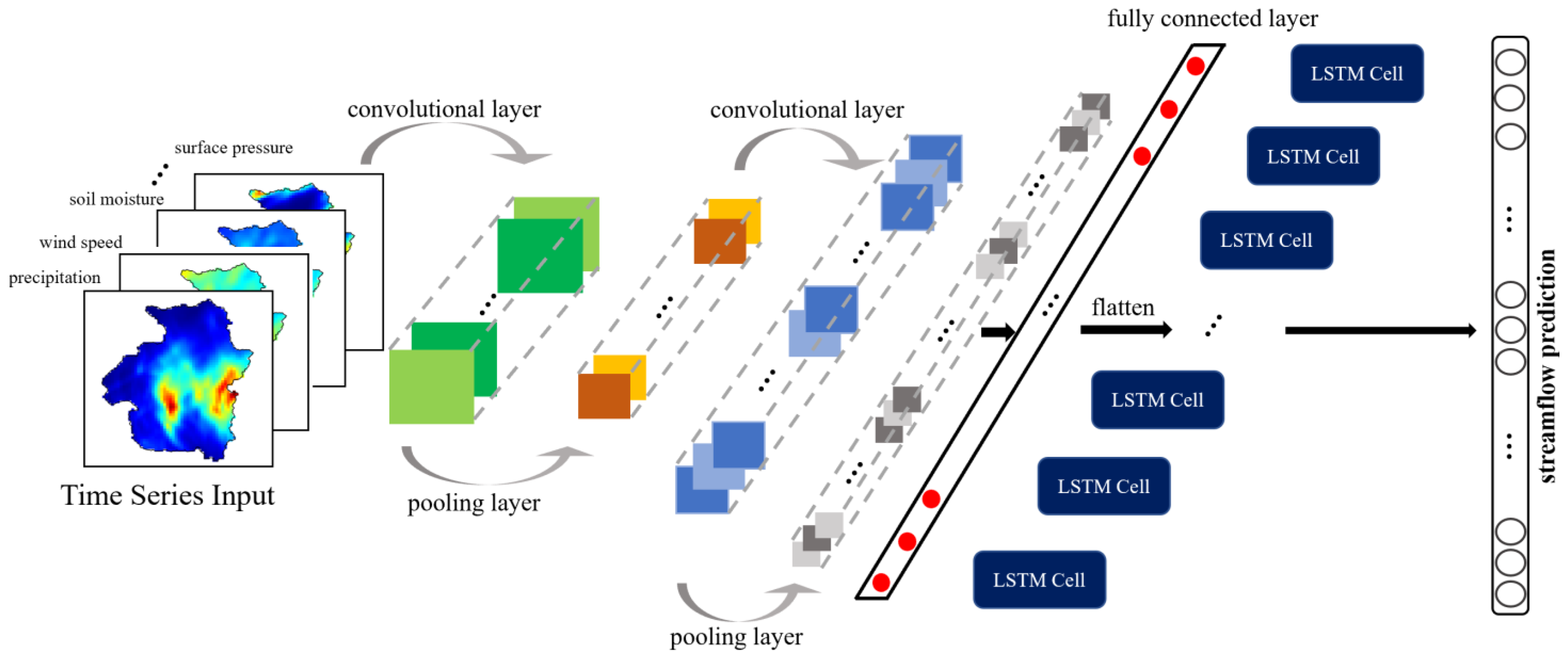
In this study, the hybrid model was designed by integrating the CNN and LSTM layers. The CNN layers extract the features from each image, and then the LSTM network captures the long short-term dependency and sequential relationships [51]. Figure 2 shows the proposed CNN-LSTM architecture in which the feature vector from the CNN layer was taken as the input to the LSTM network.

3.4. Data Preparation and Model Training

In this study, the FNL, gauge observation, and streamflow data were collected between 2007 and 2019. Because the rainfall in the catchments mainly occurred during the flood season, all the data used in this study were collected from 1 June to 30 September each year (because of a lack of observation data, the data period from 1 to 12 June 2019 was excluded). Firstly, 1° × 1° grids of FNL 6-hourly global analysis data were used to drive the WRF model. The WRF model ran for the entire flood season once a year, and the time interval of the WRF model outputs was on a daily base. Secondly, referring to the studies of Hingerl et al. [53], Fairbairn et al. [54], and Kratzert et al. [55], 16 variables were initially selected from the WRF output for use as the CNN-LSTM model input, as shown in Table 2. Then, based on the correlation between variables and with the assistance of the Gamma test, the most appropriate combinations of the WRF output variables were selected. Finally, for the selected variable combinations, CNN-LSTM models were used to simulate the streamflow and verify the effect of the Gamma test. For the purposes of training and testing, the total available data were subdivided into two nonoverlapping sets. The first data set containing data measured over 9 years (2007–2015) was used to train the CNN-LSTM model. The second data set, consisting of 4 years of data (2016–2019), was employed to test the performance of the established models. Overall, about 70% of the data were used for training and 30% for testing.
The input to the CNN-LSTM model was composed of a matrix of 81 × 81 from the innermost domain data output of the WRF. Each input variable was used as a different channel for the input. The CNN model consisted of five convolutional layers, four pooling layers, and one fully connected layer. The output from the fully connected layer was fed into an LSTM model as a one-dimensional feature vector.

3.5. Model Evaluation Criteria

In this study, the streamflow simulation performances of the data-driven models were evaluated using two criteria, i.e., root mean square error (RMSE) and Nash–Sutcliffe efficiency (NSE). The closer the RMSE value is to 0, the better the degree of model fitting. The Nash–Sutcliffe Efficiency (NSE) is used to quantitatively describe the accuracy of the hydrological model [56]. The NSE value is between 1 and negative infinity. An NSE value of 1 corresponds to a perfect match of simulated flows to observed data. A negative NSE value indicates an unacceptable model performance. These criteria were calculated as shown below:
N S E = 1 t = 1 T ( Q o t Q m t ) 2 t = 1 T ( Q o t Q o ¯ ) 2
R M S E = t = 1 T ( Q o t Q m t ) 2 T
where Q m t and Q o t represent the simulated and observed streamflow at time step t , respectively. Q o ¯ represents the means of the observed streamflow.

4. Results and Discussion

4.1. Model Input Selection Based on Gamma Test

4.1.1. Variable Selection in the Spatial Dimension

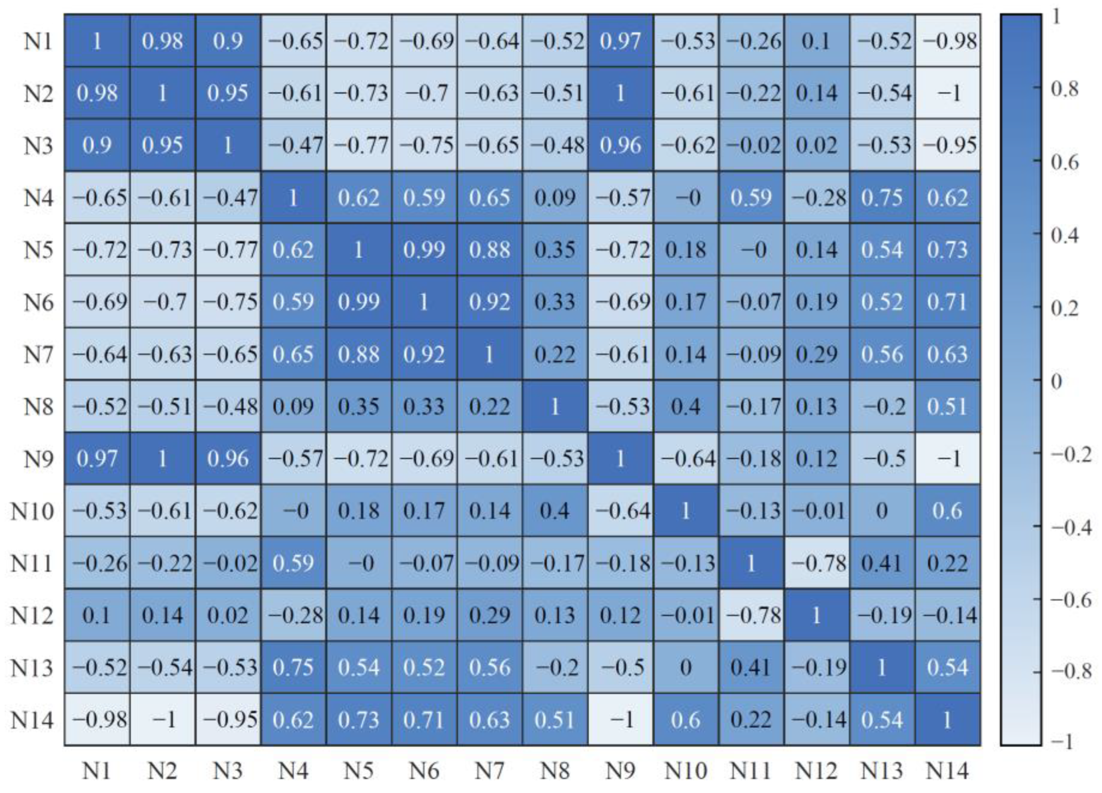
In this section, the Gamma test was used to select the combination of variables (from numbers 1–14 in Table 2) that had significant impacts on the generation of the grid runoff of the catchment, and the results of the forward and backward selection are shown in Table 3. As explained in the two-step variable selection, Variables 15 and 16 were treated as the model outputs for spatial variable selection, so these two variables are not considered in the spatial dimension. It was found that the variable combination of 2, 3, 4, 5, 7, 8, 9, 11, 12, 13, and 14 had the best performance (with the minimum | Γ | value). Correlations of the variables in the spatial dimension are also shown in Figure 3, in which it can be seen that the correlations between variables 1, 2, 3, and 9 and those between variables 5, 6, and 7 were relatively stronger (>0.90). A strong correlation indicates some degree of substitutability between the variables. Therefore, it is suggested that strongly correlated variables are not necessarily involved at the same time in the input combination.

4.1.2. Variable Selection in the Temporal Dimension

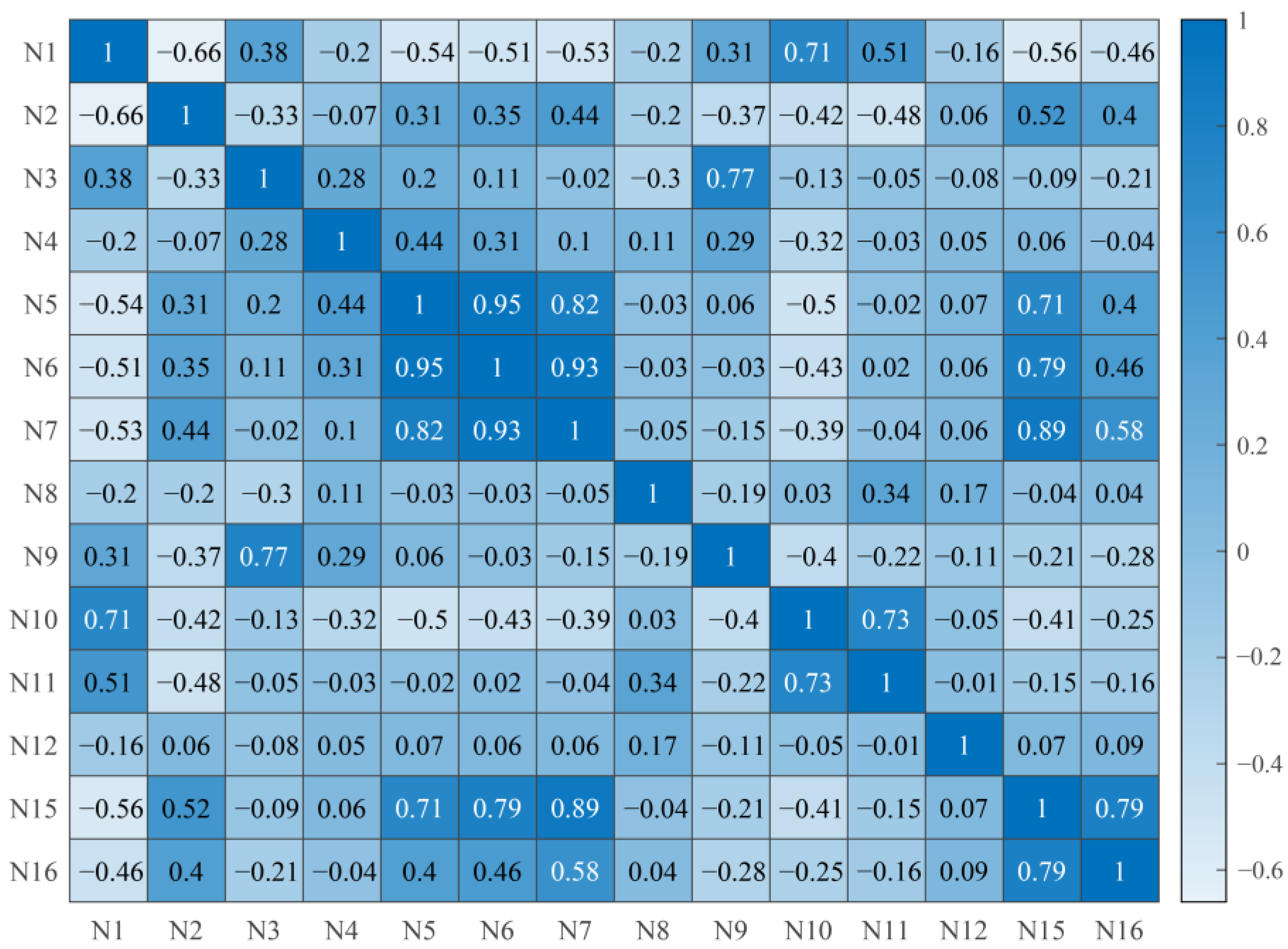
In this section, the Gamma test was used to select the combination of variables from numbers 1–13, 15, and 16 in Table 2 (13 and 14 were not taken into consideration because they were constants on a time scale) that had significant impacts on the generation of the streamflow in the temporal dimension, and the results of the forward and backward selection are shown in Table 4. The variable combination of 1, 2, 3, 4, 6, 7, 8, 15, and 16 was found to have the best performance (with the minimum | Γ | value). Variable correlations in the temporal dimension are shown in Figure 4. It can be seen that the correlations between variables 5, 6, and 7 were relatively stronger (>0.90).

4.1.3. Variable Combination Schemes as the Model Input

According to the results set out in Table 3 and Table 4, and taking the variable correlations into account, five variable combination schemes (as shown in Table 5) were finally selected as the CNN-LSTM model input. Scheme 1 contains all the variables involved in the optimal combinations in the spatial and temporal dimensions in Table 3 and Table 4. Scheme 2 contains the variables involved in the top five combinations ranked in Table 3 (3, 4, 5, 11, 12, and 14) and Table 5 (1, 3, 4, 6, 7, 8, 15, and 16). According to the correlation between variables, schemes 3, 4, and 5 were then formulated after deleting the variables with strong correlations.

4.2. Performance of the CNN-LSTM Model

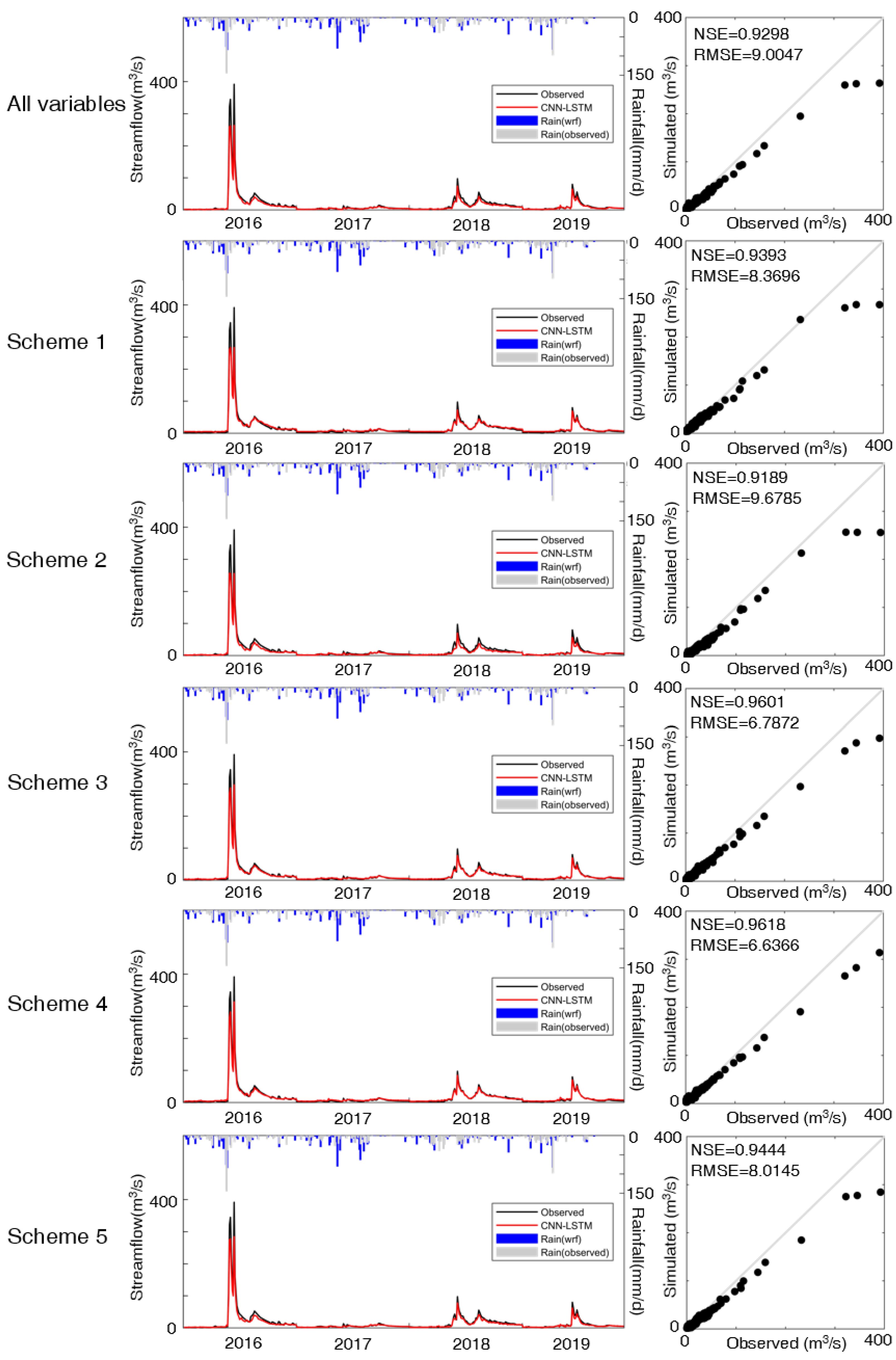
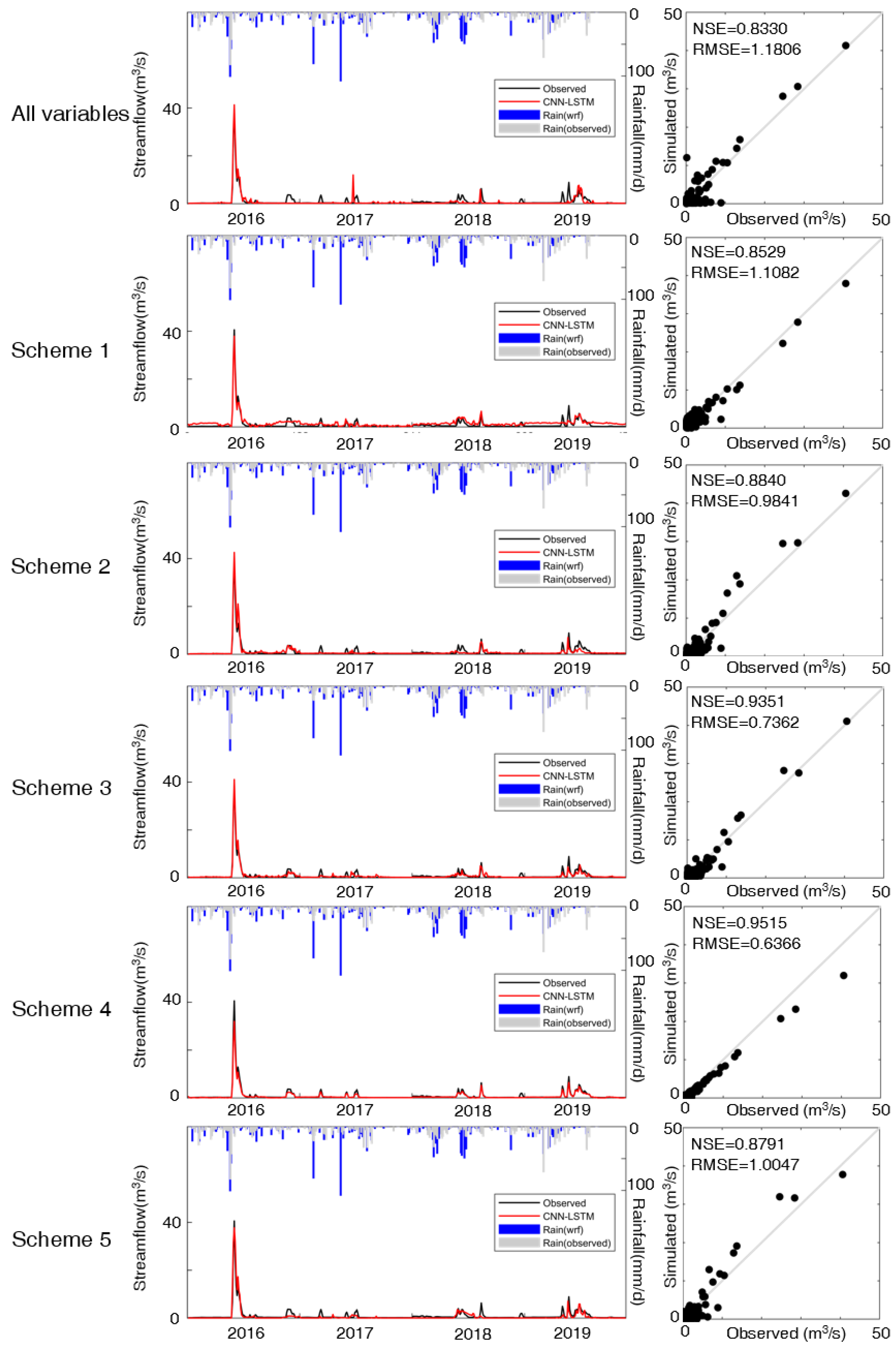
After determining the combinations of input variables, the CNN-LSTM model was used to simulate the streamflow at the catchment outlet. In this study, the CNN-LSTM models were constructed using the five schemes described in Section 4.1.3. The 16 variables in Table 2 were also used as inputs to the model for comparison purposes. The results for the Fuping and Zijingguan catchments are shown in Figure 5 and Figure 6, respectively. In Figure 5 and Figure 6, the observed rainfall refers to the average value of the rain gauge calculated by the Thiessen polygon method, and the WRF rainfall refers to the mean areal rainfall in all the catchment grids.
For the Fuping catchment (Figure 5), the performances of the CNN-LSTM models with all input combination schemes were satisfactory (NSE > 0.9). The streamflow processes were simulated accurately, and the peak times were consistent with the gauge measurements. The only exception was 2016, for which the peak discharge was inconsistent with the observed value. For all models constructed with different input schemes, the simulated peak discharges in 2016 were lower than the observed values. Scheme 4 had the best performance of all the input combination schemes, with the highest NSE value (0.9618) and the lowest RMSE value (6.6366 m3/s), and outperformed the model that included all the WRF variables.
It can be seen from Figure 5 that the peak discharges of the Fuping catchment in 2016 for all the input schemes were lower than the observed values. There are two possible reasons for this: firstly, that the WRF simulated rainfall was lower than the observed rainfall, leading to a lower simulated peak; secondly, that during the training period (2007–2015) there was no such large discharge, i.e., the maximum peak discharge in the Fuping catchment was 66.4 m3/s, whereas the peak discharge in 2016 reached 392 m3/s, leading to an unsatisfactory simulation of the peak discharge by the CNN-LSTM model.
For the Zijingguan catchment (Figure 6), the scheme 4 streamflow process was simulated accurately, and the peak time was also consistent with the gauge measurement. The rest of the schemes performed well for 2016 but showed higher error levels when simulating the streamflow processes for other years. In terms of the evaluation criteria, scheme 4 had the best NSE (0.9515) and RMSE (0.6366 m3/s) values. From the scatter diagram in Figure 6, it can be seen that scheme 4 performed best when the streamflow was small (less than 10 m3/s) but its simulated peak discharge was inferior to scheme 3.
Similar to the Fuping catchment, scheme 4 also showed the best performance of all the input schemes for the Zijingguan catchment. It can be seen from the scatter diagram in Figure 6 that the performance of scheme 4 for small discharges was better than that of other schemes, but its simulations of larger discharges were lower than the observed values. Because scheme 4 had the largest NSE value and the smallest RMSE value of all the schemes, and it can be seen from the scatter plot that the consistency of the observed and simulated streamflow of scheme 4 was superior to the other schemes, the performance of scheme 4 was considered to be the best overall. This might be due to a change in the runoff generation mechanism caused by an increase in soil moisture. The runoff generation process in the study area is accompanied by a mixed mechanism of the infiltration capacity excess and the storage capacity excess. Since the rainfall in the catchment mostly occurs in a few storm events, most of the other times the soil moisture is at a low level. During a storm, the infiltration and excess runoff generation happens first, and with the increase of the soil moisture, the storage excess then becomes dominant. However, the flow in the Zijingguan catchment is relatively small, and large flow peaks are not common. This distinctive hydrological regime is difficult to capture using the model with the current availability of training data.
For both the Fuping and Zijingguan catchments, scheme 4 had the highest NSE and the lowest RMSE value, and the number of variables in scheme 4 was relatively small (11). The lower number of input variables indicates a lower complexity of the constructed model and the faster operation speed in real-time forecasting. Considering this, scheme 4 was chosen as the best scheme for the combination of input variables for the two catchments.
In this study, the Gamma test was used to select combinations of input variables for the CNN-LSTM model in order to achieve the best performance. However, the Gamma test cannot identify the best combination for two-dimensional input data, and the selection of the variables still requires the use of correlation analysis. Nevertheless, the Gamma test had a positive effect on the modeling results and can be regarded as a helpful tool for the selection of input variables for data-driven models.
It should be mentioned that in real-time forecasting, the WRF forcing data used in this study (i.e., FNL) should be replaced with the real-time updated forecast data (e.g., GFS). Real-time forecasting is more complicated when the forcing data is updated, in normal cases, every 6 h. In such cases, the CNN-LSTM model should be restarted in accordance with the updating of the forcing data. In addition, a powerful data assimilation system of WRF-3DVar together with the streamflow updating scheme should also be implemented in order to improve the forecast skill of the hybrid system.
In the next step, on the basis of meteorological and hydrological data obtained over a longer period of time, data mining techniques can be used to conduct clustering research on historical flow processes according to different runoff mechanisms, and to identify thresholds for changes in runoff mechanisms, so that the deep learning model can be trained separately to simulate larger flood events more accurately.

5. Conclusions

In this study, a deep learning model based on a CNN-LSTM hybrid model was proposed for the simulation of daily streamflow in two different catchments of the Daqing River Basin. High-resolution (1 km) output data of the WRF model were used as the model input, and the Gamma test was shown to be highly effective in the selection of the most appropriate combination of input variables for the model. It can be seen from Table 3 that, in the spatial dimension, among the variables of each grid, precipitation is the most important variable for runoff generation in the spatial dimension. This is easy to understand, since precipitation varies the most over the study catchments and plays the most direct role in generating the streamflow. Its spatial distribution also influences the routing process and determines the time-to-peak of the flood. Similarly, it can be seen from Table 4 that, in terms of the temporal dimension, the surface runoff generated in each grid is the most important variable to the formation of the streamflow at the catchment outlet.
The CNN-LSTM model demonstrated an acceptable performance using all the WRF input variables, with NSE and RMSE values of 0.9298 and 9.0047 m3/s, respectively, in the Fuping catchment, and 0.8330 and 1.1806 m3/s, respectively, in the Zijingguan catchment. Use of the Gamma test further improved the performance of the CNN-LSTM model. Using the best-performing combination scheme indicated by the model (scheme 4), the NSE increased to 0.9618 and the RMSE decreased to 6.6366 m3/s for the Fuping catchment, and for the Zijingguan catchment the NSE increased to 0.9515 and the RMSE decreased to 0.6366 m3/s. These results indicate the feasibility of using the WRF-downscaled high-resolution data for streamflow simulation in data-limited or ungauged catchments.
In this study, the Gamma test selection was based on data collected in the Fuping catchment. Scheme 4, which performed best in Fuping, also showed the best performance in Zijingguan, indicating that the selected input combination schemes may be applicable to catchments of the same scale and with similar hydrometeorological regimes. In the next step, we will add data from similar small-scale catchments in the surrounding area and try to build a regional universal streamflow model.
With the advantages of high resolution and consideration of detailed physical processes, regional climate models have become key tools for climate prediction. Taking the outcome of a regional climate model as the forcing data and using deep learning approaches, future extreme flood events under different scenarios can be predicted and water resource change trends can be assessed. This study provides an important reference for hydrometeorological modeling in ungauged or data-limited catchments, which has significance for flood control planning and management of water resources in the context of future climate change.

Author Contributions

Conceptualization, Y.W. and J.L.; methodology, Y.W., J.L. and F.Y.; software, Y.W.; validation, S.Z. and L.X.; formal analysis, Y.W. and J.L.; investigation, Y.W. and L.X.; writing—original draft preparation, Y.W. and J.L.; writing—review and editing, Y.W. and J.L.; visualization, Y.W. and L.X.; funding acquisition, J.L. All authors have read and agreed to the published version of the manuscript.

Funding

This research was funded by the National Natural Science Foundation of China (51822906), the Major Science and Technology Program for Water Pollution Control and Treatment (2018ZX07110001), and the National Key Research and Development Project (2019YFC0409104).

Data Availability Statement

The data presented in this study are available on request from the corresponding author.

Conflicts of Interest

The authors declare no conflict of interest.

References

  1. Emerton, R.E.; Stephens, E.M.; Pappenberger, F.; Pagano, T.C.; Weerts, A.H.; Wood, A.W.; Salamon, P.; Brown, J.D.; Hjerdt, N.; Donnelly, C.; et al. Continental and global scale flood forecasting systems. Wiley Interdiscip. Rev. Water 2016, 3, 391–418. [Google Scholar] [CrossRef] [Green Version]
  2. Yaseen, Z.M.; Sulaiman, S.O.; Deo, R.C.; Chau, K.W. An enhanced extreme learning machine model for river flow forecasting: State-of-the-art, practical applications in water resource engineering area and future research direction. J. Hydrol. 2018, 569, 387–408. [Google Scholar] [CrossRef]
  3. Wang, W.; Vrijling, J.K.; Van Gelder, P.H.; Ma, J. Testing for nonlinearity of streamflow processes at different timescales. J. Hydrol. 2006, 322, 247–268. [Google Scholar] [CrossRef]
  4. Skamarock, W. A Description of the Advanced Research WRF Version 3; NCAR Tech. Note; NCAR/TN-475+ STR; University Corporation for Atmospheric Research: Boulder, CO, USA, 2008. [Google Scholar]
  5. Bass, B.; Rahimi, S.; Goldenson, N.; Hall, A.; Norris, J.; Lebow, Z.J. Achieving Realistic Runoff in the Western United States with a Land Surface Model Forced by Dynamically Downscaled Meteorology. J. Hydrometeorol. 2023, 24, 269–283. [Google Scholar] [CrossRef]
  6. Tyson, C.; Longyang, Q.; Neilson, B.T.; Zeng, R.; Xu, T. Effects of Meteorological Forcing Uncertainty on High-Resolution Snow Modeling and Streamflow Prediction in a Mountainous Karst Watershed. J. Hydrol. 2023, 619, 129304. [Google Scholar] [CrossRef]
  7. Naabil, E.; Lamptey, B.L.; Arnault, J.; Olufayo, A.; Kunstmann, H. Water resources management using the WRF-Hydro modelling system: Case-study of the Tono dam in West Africa. J. Hydrol. Reg. Stud. 2017, 12, 196–209. [Google Scholar] [CrossRef]
  8. Wang, J.; Bao, W.; Gao, Q.; Si, W.; Sun, Y. Coupling the Xinanjiang model and wavelet-based random forests method for improved daily streamflow simulation. J. Hydroinformatics 2021, 23, 589–604. [Google Scholar] [CrossRef]
  9. Gu, Y.; Peng, D.; Deng, C.; Zhao, K.; Pang, B.; Zuo, D. Atmospheric–hydrological modeling for Beijing’s sub-center based on WRF and SWMM. Urban Clim. 2022, 41, 101066. [Google Scholar] [CrossRef]
  10. Nourani, V. An emotional ANN (EANN) approach to modeling rainfall-runoff process. J. Hydrol. 2017, 544, 267–277. [Google Scholar] [CrossRef]
  11. Ni, L.; Wang, D.; Singh, V.P.; Wu, J.; Wang, Y.; Tao, Y.; Zhang, J. Streamflow and rainfall forecasting by two long short-term memory-based models. J. Hydrol. 2020, 583, 124296. [Google Scholar] [CrossRef]
  12. Choi, J.; Lee, J.; Kim, S. Utilization of the Long Short-Term Memory network for predicting streamflow in ungauged basins in Korea. Ecol. Eng. 2022, 182, 106699. [Google Scholar] [CrossRef]
  13. Wegayehu, E.B.; Muluneh, F.B. Short-Term Daily Univariate Streamflow Forecasting Using Deep Learning Models. Adv. Meteorol. 2022, 2022, 1860460. [Google Scholar] [CrossRef]
  14. Xiang, Z.; Yan, J.; Demir, I. A rainfall-runoff model with LSTM-based sequence-to-sequence learning. Water Resour. Res. 2020, 56, e2019WR025326. [Google Scholar] [CrossRef]
  15. Thapa, S.; Zhao, Z.; Li, B.; Lu, L.; Fu, D.; Shi, X.; Tang, B.; Qi, H. Snowmelt-driven streamflow prediction using machine learning techniques (LSTM, NARX, GPR, and SVR). Water 2020, 12, 1734. [Google Scholar] [CrossRef]
  16. Krizhevsky, A.; Sutskever, I.; Hinton, G. ImageNet classification with deep convolutional neural networks. Commun. Acm 2017, 60, 84–90. [Google Scholar] [CrossRef] [Green Version]
  17. LeCun, Y.; Bengio, Y.; Hinton, G. Deep learning. Nature 2015, 521, 436–444. [Google Scholar] [CrossRef]
  18. Lei, X.; Pan, H.; Huang, X. A dilated CNN model for image classification. IEEE Access 2019, 7, 124087–124095. [Google Scholar] [CrossRef]
  19. Poma, X.S.; Riba, E.; Sappa, A. Dense extreme inception network: Towards a robust CNN model for edge detection. In Proceedings of the IEEE/CVF Winter Conference on Applications of Computer Vision, Snowmass Village, CO, USA, 2–5 March 2020. [Google Scholar]
  20. AlBdairi, A.J.A.; Xiao, Z.; Alkhayyat, A.; Humaidi, A.J.; Fadhel, M.A.; Taher, B.H.; Alzubaidi, L.; Santamaría, J.; Al-Shamma, O. Face Recognition Based on Deep Learning and FPGA for Ethnicity Identification. Appl. Sci. 2022, 12, 2605. [Google Scholar] [CrossRef]
  21. Van, S.P.; Le, H.M.; Thanh, D.V.; Dang, T.D.; Loc, H.H.; Anh, D.T. Deep learning convolutional neural network in rainfall–runoff modelling. J. Hydroinformatics 2020, 22, 541–561. [Google Scholar] [CrossRef] [Green Version]
  22. Wang, Y.; Fang, Z.; Hong, H.; Peng, L. Flood susceptibility mapping using convolutional neural network frameworks. J. Hydrol. 2020, 582, 124482. [Google Scholar] [CrossRef]
  23. Barzegar, R.; Aalami, M.T.; Adamowski, J. Coupling a hybrid CNN-LSTM deep learning model with a boundary corrected maximal overlap discrete wavelet transform for multiscale lake water level forecasting. J. Hydrol. 2021, 598, 126196. [Google Scholar] [CrossRef]
  24. Li, P.; Zhang, J.; Krebs, P. Prediction of flow based on a CNN-LSTM combined deep learning approach. Water 2022, 14, 993. [Google Scholar] [CrossRef]
  25. Tran, H.; Leonarduzzi, E.; De la Fuente, L.; Hull, R.B.; Bansal, V.; Chennault, C.; Gentine, P.; Melchior, P.; Condon, L.E.; Maxwell, R.M. Development of a Deep Learning Emulator for a Distributed Groundwater–Surface Water Model: ParFlow-ML. Water 2021, 13, 3393. [Google Scholar] [CrossRef]
  26. Koncar, N. Optimisation Methodologies for Direct Inverse Neurocontrol. Ph.D. Thesis, University of London, London, UK, 1997. [Google Scholar]
  27. Malik, A.; Tikhamarine, Y.; Souag-Gamane, D.; Kisi, O.; Pham, Q.B. Support vector regression optimized by meta-heuristic algorithms for daily streamflow prediction. Stoch. Environ. Res. Risk Assess. 2020, 34, 1755–1773. [Google Scholar] [CrossRef]
  28. Hassan, M.; Hassan, I. Improving Artificial Neural Network Based Streamflow Forecasting Models through Data Preprocessing. KSCE J. Civ. Eng. 2021, 25, 3583–3595. [Google Scholar] [CrossRef]
  29. Panahi, F.; Ehteram, M.; Ahmed, A.N.; Huang, Y.F.; Mosavi, A.; El-Shafie, A. Streamflow prediction with large climate indices using several hybrid multilayer perceptrons and copula Bayesian model averaging. Ecol. Indic. 2021, 133, 108285. [Google Scholar] [CrossRef]
  30. Zhuo, L.; Han, D. Multi-source hydrological soil moisture state estimation using data fusion optimisation. Hydrol. Earth Syst. Sci. 2017, 21, 3267–3285. [Google Scholar] [CrossRef] [Green Version]
  31. Tian, J.; Li, C.; Liu, J.; Yu, F.; Cheng, S.; Zhao, N.; Wan Jaafar, W.Z. Groundwater Depth Prediction Using Data-Driven Models with the Assistance of Gamma Test. Sustainability 2016, 8, 1076. [Google Scholar] [CrossRef] [Green Version]
  32. Cardoso, R.M.; Soares PM, M.; Miranda PM, A.; Belo-Pereira, M. WRF high resolution simulation of Iberian mean and extreme precipitation climate. Int. J. Climatol. 2013, 33, 2591–2608. [Google Scholar] [CrossRef]
  33. Toride, K.; Iseri, Y.; Duren, A.M.; England, J.F.; Kavvas, M.L. Evaluation of physical parameterizations for atmospheric river induced precipitation and application to long-term reconstruction based on three reanalysis datasets in Western Oregon. Sci. Total Environ. 2018, 658, 570–581. [Google Scholar] [CrossRef]
  34. Lin, Y.L.; Farley, R.D.; Orville, H.D. Bulk parameterization of the snow field in a cloud model. J. Clim. Appl. Meteorol. 1983, 22, 1065–1092. [Google Scholar] [CrossRef]
  35. Mlawer, E.J.; Taubman, S.J.; Brown, P.D.; Iacono, M.J.; Clough, S.A. Radiative transfer for inhomogeneous atmospheres: RRTM, a vali-dated correlated-k model for the longwave. J. Geophys. Res. Atmos. 1997, 102, 16663–16682. [Google Scholar] [CrossRef] [Green Version]
  36. Dudhia, J. Numerical study of convection observed during the winter monsoon experiment using a mesoscale two-dimensional model. J. Atmos. Sci. 1989, 46, 3077–3107. [Google Scholar] [CrossRef]
  37. Chen, F.; Dudhia, J. Coupling an advanced land surface-hydrology model with the Penn State-NCAR MM5 modeling system. Part I: Model implementation and sensitivity. Mon. Weather Rev. 2001, 129, 569–585. [Google Scholar] [CrossRef]
  38. Hong, S.Y.; Noh, Y.; Dudhia, J. A new vertical diffusion package with an explicit treatment of entrainment processes. Mon. Weather Rev. 2006, 134, 2318–2341. [Google Scholar] [CrossRef] [Green Version]
  39. Kain, J.S. The Kain–Fritsch convective parameterization: An update. J. Appl. Meteorol. 2004, 43, 170–181. [Google Scholar] [CrossRef]
  40. Tian, J.; Liu, J.; Wang, J.; Li, C.; Yu, F.; Chu, Z. A spatio-temporal evaluation of the WRF physical parameterisations for numerical rainfall simulation in semi-humid and semi-arid catchments of northern China. Atmos. Res. 2017, 191, 141–155. [Google Scholar] [CrossRef]
  41. Liu, Y.; Liu, J.; Li, C.; Yu, F.; Wang, W.; Qiu, Q. Parameter sensitivity analysis of the WRF-hydro modeling system for streamflow simulation: A case study in semi-humid and semi-arid Catchments of Northern China. Asia-Pac. J. Atmos. Sci. 2021, 57, 451–466. [Google Scholar] [CrossRef]
  42. Stefánsson, A.; Končar, N.; Jones, A.J. A note on the gamma test. Neural Comput. Appl. 1997, 5, 131–133. [Google Scholar] [CrossRef]
  43. Evans, D.; Jones, A.J. A proof of the Gamma test. Proc. R. Soc. Lond. Ser. A 2002, 458, 2759–2799. [Google Scholar] [CrossRef]
  44. Tsui, A.P.; Jones, A.J.; Guedes de Oliveira, A. The construction of smooth models using irregular embeddings determined by a gamma test analysis. Neural Comput. Appl. 2002, 10, 318–329. [Google Scholar] [CrossRef]
  45. Wan Jaafar, W.Z.; Han, D. Variable Selection Using the Gamma Test Forward and Backward Selections. J. Hydrol. Eng. 2012, 17, 182–190. [Google Scholar] [CrossRef]
  46. LeCun, Y.; Bottou, L.; Bengio, Y.; Haffner, P. Gradient-based learning applied to document recognition. Proc. IEEE 1998, 86, 2278–2324. [Google Scholar] [CrossRef] [Green Version]
  47. Lawrence, S.; Giles, C.L.; Tsoi, A.C.; Back, A.D. Face Recognition: A Convolutional Neural-Network Approach. IEEE Trans. Neural Netw. 1997, 8, 98–113. [Google Scholar] [CrossRef] [Green Version]
  48. Hochreiter, S.; Schmidhuber, J. Long short-term memory. Neural Comput. 1997, 9, 1735–1780. [Google Scholar] [CrossRef]
  49. Gers, F.A.; Schmidhuber, J.; Cummins, F. Continual prediction using LSTM with forget gates. In Neural Nets WIRN Vietri-99; Springer: London, UK, 1999; pp. 133–138. [Google Scholar]
  50. Wu, Q.; Lin, H. Daily urban air quality index forecasting based on variational mode decomposition, sample entropy and LSTM neural network. Sustain. Cities Soc. 2019, 50, 101657. [Google Scholar] [CrossRef]
  51. Fang, Z.; Wang, Y.; Peng, L.; Hong, H. Predicting flood susceptibility using LSTM neural networks. J. Hydrol. 2021, 594, 125734. [Google Scholar] [CrossRef]
  52. Li, X.; Xu, W.; Ren, M.; Jiang, Y.; Fu, G. Hybrid CNN-LSTM models for river flow prediction. Water Supply 2022, 22, 4902–4919. [Google Scholar] [CrossRef]
  53. Hingerl, L.; Kunstmann, H.; Wagner, S.; Mauder, M.; Bliefernicht, J.; Rigon, R. Spatio-temporal variability of water and energy fluxes–a case study for a mesoscale catchment in pre-alpine environment. Hydrol. Process. 2016, 30, 3804–3823. [Google Scholar] [CrossRef] [Green Version]
  54. Fairbairn, D.; Barbu, A.L.; Napoly, A.; Albergel, C.; Mahfouf, J.F.; Calvet, J.C. The effect of satellite-derived surface soil moisture and leaf area index land data assimilation on streamflow simulations over France. Hydrol. Earth Syst. Sci. 2017, 21, 2015–2033. [Google Scholar] [CrossRef] [Green Version]
  55. Kratzert, F.; Klotz, D.; Brenner, C.; Schulz, K.; Herrnegger, M. Rainfall–runoff modelling using long short-term memory (LSTM) networks. Hydrol. Earth Syst. Sci. 2018, 22, 6005–6022. [Google Scholar] [CrossRef] [Green Version]
  56. Nash, J.E.; Sutcliffe, J.V. River flow forecasting through conceptual models part I—A discussion of principles. J. Hydrol. 1970, 10, 282–290. [Google Scholar] [CrossRef]
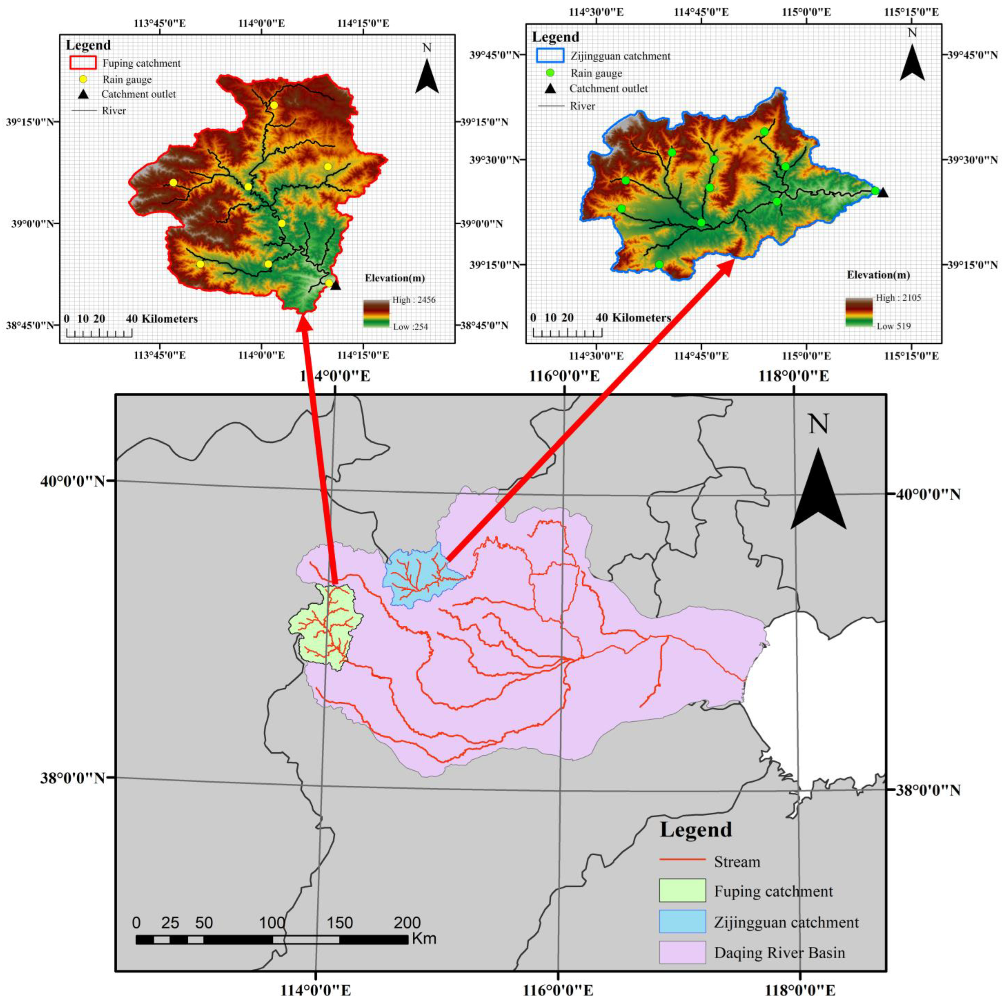
Figure 1. Locations of the study area and the catchments covered by the WRF innermost domain.
Water 15 01422 g001
Figure 2. Structure of the convolutional neural network (CNN) integrated with the long short-term memory (LSTM) network used in this study [52].
Water 15 01422 g002
Figure 3. Heatmap of the variable correlations in the spatial dimension.
Water 15 01422 g003
Figure 4. Heatmap of the variable correlations in the temporal dimension.
Water 15 01422 g004
Figure 5. Performance of the CNN-LSTM model in the Fuping catchment during 2016–2019.
Water 15 01422 g005
Figure 6. Performance of the CNN-LSTM model in the Zijingguan catchment during 2016–2019.
Water 15 01422 g006
Table 1. Configurations of the WRF model.
SubjectChosen OptionSubjectChosen Option
Forcing data6-hourly FNLFuping domain center39.0856 N, 113.9899 E
Time step150 sZijingguan domain center39.4430 N, 114.8274 E
Horizontal resolutionDom1: 27 kmDomain areaDom1: 613,089 km2
Dom2: 9 kmDom2: 88,209 km2
Dom3: 3 kmDom3: 18,225 km2
Dom4: 1 kmDom4: 6561 km2
Projection LambertWRF output interval1 day
Table 2. WRF downscaled variables used as the CNN-LSTM model inputs.
No.VariablesNo.Variables
1Surface skin temperature9Downward long wave flux
2Surface pressure10Downward short wave flux
3Specific humidity11Latent heat flux
4Precipitation12Albedo
5Soil moisture (0–10 cm)13Orographic variance
6Soil moisture (10–40 cm)14Terrain height
7Soil moisture (40–100 cm)15Surface runoff
8Wind speed16Underground runoff
Table 3. Backward and forward selection of variables in the spatial dimension using the Gamma test.
RankingsCombination of VariablesIndex Removed/Added Γ GradientStandard Error V r a t i o
171,2,3,4,5,6,7,8,9,10,11,12,13,14None−0.001850.093750.00139−0.00739
71,2,3,4,5,6,7,8,9,11,12,13,14100.000460.097470.000790.00182
61,2,3,4,5,7,8,9,11,12,13,146−0.000300.117480.00106−0.00121
12,3,4,5,7,8,9,11,12,13,1410.000040.119310.000680.00016
32,3,4,5,7,8,9,11,12,14130.000090.141110.000670.00035
82,3,4,5,7,8,11,12,1490.000540.141980.000990.00217
122,3,4,5,7,8,11,12140.001260.140240.000870.00504
142,4,5,7,8,11,1230.001370.161440.001070.00547
152,4,5,7,8,12110.001640.187160.001020.00655
202,4,5,8,1270.002900.275720.000920.01160
222,4,5,1280.003670.412710.000450.01470
242,4,5120.008620.532730.001010.03448
254,520.023050.880200.001320.09219
27450.05331−13.291600.001500.21322
264,540.023050.880200.001320.09219
233,4,530.006900.587070.000830.02761
213,4,5,12120.003150.418900.000740.01259
193,4,5,12,14140.002480.354390.001020.00993
163,4,5,10,12,14100.001760.272340.000500.00704
111,3,4,5,10,12,1410.001160.257180.000670.00464
131,3,4,5,10,11,12,14110.001330.211650.001380.00530
51,3,4,5,6,10,11,12,1460.000140.167230.001330.00058
21,3,4,5,6,8,10,11,12,1480.000080.134370.000920.00030
41,3,4,5,6,7,8,10,11,12,147−0.000130.104440.00085−0.00054
91,3,4,5,6,7,8,9,10,11,12,149−0.000710.104680.00086−0.00284
101,3,4,5,6,7,8,9,10,11,12,13,1413−0.000910.090540.00146−0.00364
181,2,3,4,5,6,7,8,9,10,11,12,13,142−0.001850.093750.00139−0.00739
Table 4. Backward and forward selection of variables in the temporal dimension using the Gamma test.
RankingsCombination of VariablesIndex Removed/Added Γ GradientStandard Error V r a t i o
231,2,3,4,5,6,7,8,9,10,11,12,15,16None0.04340.11340.01270.1737
171,2,3,4,5,6,7,8,9,11,12,15,16100.02630.14250.01340.1052
121,2,3,4,5,6,7,8,11,12,15,1690.02170.15930.01160.0867
51,2,3,4,5,6,7,8,12,15,16110.00980.19260.00890.0392
21,2,3,4,6,7,8,12,15,1650.00470.22610.01450.0187
11,2,3,4,6,7,8,15,1612−0.00090.35600.0140−0.0035
81,3,4,6,7,8,15,1620.01520.40260.00720.0606
131,3,6,7,8,15,1640.02170.50870.01150.0867
151,3,6,7,15,1680.02220.89770.01280.0887
203,6,7,15,1610.03271.42360.00770.1309
256,7,15,1630.04453.12990.00590.1779
227,15,1660.03758.40310.00730.1499
267,15160.048419.27610.00540.1935
271570.0786669.59490.01930.3142
1812,15120.03020.61410.01060.1206
1012,15,16160.02150.58120.01360.0859
77,12,15,1670.01500.35200.00520.0599
164,7,12,15,1640.02230.30430.00980.0891
191,4,7,12,15,1610.03080.31040.00560.1231
211,4,6,7,12,15,1660.03430.23570.00770.1371
141,3,4,6,7,12,15,1630.02180.27270.00930.0870
91,3,4,5,6,7,12,15,1650.01520.26960.00600.0608
31,3,4,5,6,7,8,12,15,1680.00770.23710.00720.0309
61,2,3,4,5,6,7,8,12,15,1620.00980.19260.00890.0392
41,2,3,4,5,6,7,8,10,12,15,16100.00940.18010.00940.0374
111,2,3,4,5,6,7,8,10,11,12,15,16110.02170.15930.01160.0867
241,2,3,4,5,6,7,8,9,10,11,12,15,1690.04340.11340.01270.1737
Table 5. Variable combination schemes for the CNN-LSTM model input.
Scheme IDCombination of Variables
11,2,3,4,5,6,7,8,9,11,12,13,14,15,16
21,3,4,5,6,7,8,11,12,14,15,16
32,4,5,6,7,8,11,12,14,15,16
41,3,4,5,7,8,11,12,14,15,16
52,4,5,7,8,11,12,14,15,16
Disclaimer/Publisher’s Note: The statements, opinions and data contained in all publications are solely those of the individual author(s) and contributor(s) and not of MDPI and/or the editor(s). MDPI and/or the editor(s) disclaim responsibility for any injury to people or property resulting from any ideas, methods, instructions or products referred to in the content.