Article

Evaluation of Different Methods on the Estimation of the Daily Crop Coefficient of Winter Wheat

1
College of Hydrology and Water Resources, Hohai University, Nanjing 210024, China
2
Nanjing Hydraulic Research Institute, Nanjing 210029, China
3
Wudaogou Hydrologic Experimental Station, Water Resources Research Institute of Anhui Province (Huai Committee of the Ministry of Water Resources), Bengbu 233700, China
*
Author to whom correspondence should be addressed.
Water 2023, 15(7), 1395; https://doi.org/10.3390/w15071395
Submission received: 15 February 2023 / Revised: 23 March 2023 / Accepted: 30 March 2023 / Published: 4 April 2023
(This article belongs to the Topic Hydrology and Water Resources in Agriculture and Ecology)

Abstract

:
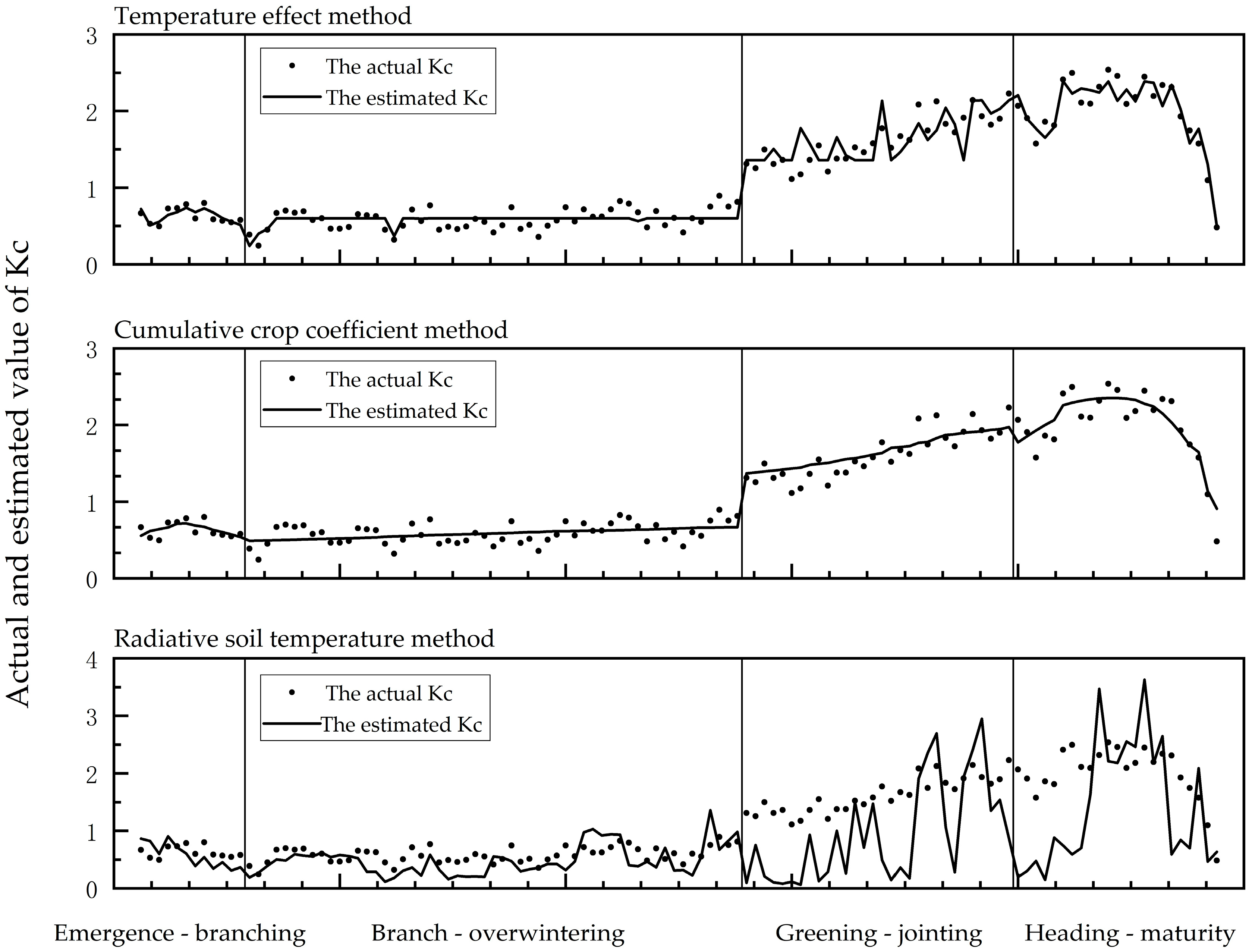
Various methods have been developed to estimate daily crop coefficients, but their performance varies. In this paper, a comprehensive evaluation was conducted to estimate the crop coefficient of winter wheat in four growth stages based on the observed data of weighing-type lysimeters and the high-precision automatic weather station in the Wudaogou Hydrological Experimental Station from 2018 to 2019. The three methods include the temperature effect method, the cumulative crop coefficient method, and the radiative soil temperature method. Our results suggest that the performance of these methods was different in each individual growth stage. The temperature effect method was better in the emergence-branching (RMSE = 0.06, r = 0.80) and heading-maturity stages (RMSE = 0.16, r = 0.94) because the temperature is suitable for crop growth during most of these two periods. The cumulative crop coefficient method was better in the greening-jointing (RMSE = 0.16, r = 0.88) and heading-maturity stages (RMSE = 0.20, r = 0.91) because this method is closely related to crop growth, which is vigorous during these two stages. The radiative soil temperature method was better in the emergence-branching (RMSE = 0.20, r = 0.35) and branch-overwintering stages (RMSE = 0.25, r = 0.52) as the energy balance can be ensured by the relatively high level of the effective energy during these periods. By comparing the estimation accuracy indices of the three methods, we found that the temperature effect method performed the best during the emergence-branching stage (RMSE = 0.06, MAE = 0.06, r = 0.80, dIA = 0.88), branch-overwintering stage (RMSE = 0.13, MAE = 0.11, r = 0.44, dIA = 0.55), and heading-maturity stage (RMSE = 0.16, MAE = 0.13, r = 0.94, dIA = 0.97), while the cumulative crop coefficient method performed best during the greening-jointing stage (RMSE = 0.16, MAE = 0.13, r = 0.88, dIA = 0.89). Based on this result, an integrated modelling procedure was proposed by applying the best method in each growth stage, which provides higher simulation precision than any single method. When the best method was adopted in each growth stage, the estimated accuracy of the whole growth process was RMSE = 0.13, MAE = 0.09, r = 0.98, dIA = 0.99.

1. Introduction

According to data released by the Food and Agriculture Organization (FAO), the FAO Food Price Index in 2021 reached a 10-year high, and the incidence of moderate or severe food insecurity in the world increased from 22.6% in 2014 to 30.4% in 2020. In 2020, an estimated 720 to 811 million people, or 9.5 to 10.7 percent of the global population, will face food insecurity [1]. Agricultural irrigation accounts for 87% of total water use [2], but water resources are increasingly in short supply under the pressure of climate change and population growth [3]. Accurate estimation of crop water demand is of great significance for rational allocation of water resources.
Wheat is one of the main crops grown and eaten worldwide [4]. From 2011 to 2020, the global average annual planting area reached 219 million hectares, with an annual yield of 733 million tons [5]. Wheat is the second main crop in China [6]; the wheat output of China accounts for approximately 18% of the world’s output (ranking first in the world), and the sown area accounts for approximately 10% of that of the world [7]. Winter wheat is sown from October to November and harvested from May to June of the following year. Planting is performed in dry conditions with little rainfall. Accurate estimation of the daily evapotranspiration and crop coefficient of winter wheat is conducive to the formulation of accurate irrigation schemes to improve the yield of winter wheat and save water resources [8].
Evapotranspiration is an important link in the hydrological cycle and is involved in the surface energy balance and water balance [9]. The crop coefficient is the ratio of actual evapotranspiration and reference evapotranspiration of crops, reflecting the influence of soil, vegetation, and hydrometeorological conditions on evapotranspiration and is often used to calculate crop water requirements [10]. Finding a suitable crop coefficient estimation method is of great significance for further estimating actual evapotranspiration, making irrigation plans, and efficiently utilizing water resources.
Domestic and foreign scholars have performed much research on crop coefficient estimation methods. In the crop coefficient estimation method recommended by FAO, the basic crop coefficient constant is obtained by plotting tabulated values and drawing the crop coefficient curve with a simplified straight-line connection at each growth stage. Finally, the daily crop coefficient value is modified according to wind speed and humidity. This method has been widely adopted and is very convenient for practical application. Er-Raki et al. [11] directly used the basic crop coefficient provided by the FAO Irrigation and Drainage Paper No. 56 (FAO-56) to calculate the soil surface vegetation coverage. Vu et al. [12] compared the crop coefficient recommended by the FAO-56 with the field monitoring value and found that the applicability of the recommended value of FAO-56 was affected by crop variety and growth stage. Ali et al. [13] simulated the Kc curve using four crop coefficient estimation methods, including the FAO-56 recommendation method. Many scholars estimate the crop coefficient according to the crop growth character index and calculate the crop coefficient by measuring the leaf area, plant height, vegetation index, etc. The daily scale is usually obtained by linear interpolation. This method of estimation has strong physical significance and high accuracy. Spiliotopoulos et al. [14] estimated crop coefficients based on the vegetation index using mapping ET of high resolution and internalized calibration models. Zhang et al. [15] established two Ks regression models for crop coefficient inversion and found that the model established by TCARI/RDVI had a better correlation with the crop coefficient. Park et al. [8] estimated crop coefficients for cropland and mixed forest based on the normalized vegetation index, leaf area index, and soil moisture.
The above methods use the same method to estimate the crop coefficient at each growth stage, but the growth of crops at different growth stages and the hydrometeorological factors closely related to their growth are different. It is difficult to obtain satisfactory results with a single method, so it is necessary to select the best method to estimate the crop coefficient at different growth stages. Based on the temperature effect, Wang et al. [16] established a daily crop coefficient estimation model of winter wheat and summer maize with a high fitting degree and found that the estimation effect of each growth stage was different. Tang et al. [17] conducted a remote sensing study by UAV and found that there was a good linear correlation between biomass and the cumulative crop coefficient and cumulative transpiration in different treatment areas. Kool et al. [18] evaluated the dual source energy balance (TSEB) model using net radiation, soil heat flux, and surface temperature. Paulino et al. [19] proposed an empirical model based on linear multiple regression to estimate the number of fruits per plant of two sweet oranges and concluded that the estimates of the model varied greatly in the three growth stages. At present, most related studies from both China and abroad focus on crop coefficient estimation methods. Few studies have compared the differences in crop coefficient estimation methods in different growth stages and provided the best estimation methods in each growth stage. In this paper, we attempt to select three methods, the temperature effect method, cumulative crop coefficient method, and radiative soil temperature method, to compare and analyse their estimation results to provide the best estimation method of crop coefficients in different growth stages and provide a basis for the accurate calculation of evapotranspiration in each growth stage.

2. Materials and Methods

2.1. Experimental Area Profile

The measured experimental data of the Wudaogou hydrological experimental station were used. The station is located in Guzhen County (33°09′ N, 117°21′ E), Bengbu City, Anhui Province, in the southern Huaibei Plain, covering an area of 27,000 square meters. It is affected by a subtropical humid monsoon climate and temperate subhumid monsoon climate, with rain and heat at the same time. The rainfall in the area where the experimental station is located varies greatly from year to year and is unevenly distributed within the year. A total of 61.8% of the annual rainfall is concentrated in the flood season (from June to September). The main soil types in the experimental area are sandy ginger black soil and yellow tidal soil, and the main crops are wheat, corn, and soybean. There are 62 sets of nonweighing ground lysimeters and 10 sets of large-scale weighing lysimeters in the station, which can record submersible evaporation, soil moisture, and evapotranspiration. A high-precision weather station is set up about 50 m south of the weighing lysimeters to automatically monitor net radiation, soil heat flux, air temperature, wind speed, and other hydrometeorological elements every 10 min.
According to the measured hydrometeorological data from 1986 to 2021, the average annual temperature is 15.2 °C, the average annual rainfall is 929.5 mm, the average annual flood season rainfall is 582.4 mm, the average annual evaporation is 931.9 mm, the average annual relative humidity is 79.28%, the average annual sunshine duration is 1723.6 h, the average annual wind speed is 1.6 m/s, the annual average surface temperature is 18.4 °C, the annual average soil temperature at 10 cm is 16.6 °C, the maximum temperature is 41.5 °C, and the minimum temperature is −22.7 °C.

2.2. Experimental Facilities and Data Selection

The difference in the three crop coefficient estimation methods at different growth stages and daily scales was studied by using a large-scale lysimeter. The winter wheat relies on rainfall. The lysimeter model is FR101A, the resolution is 0.025 mm, the soil column height is 4.0 m, the diameter area is 2.0 square meters, and the weight data are automatically collected every 10 min. The depth of the groundwater level in the shallow buried area of the Huaibei Plain is 1 to 3 m [20], and the root system of winter wheat is concentrated within 1 m [21]. Therefore, experimental data from a lysimeter with a burial depth of 1.0 m and measured data from high-precision weather stations were selected from 11 November 2018 to 4 June 2019.

2.3. Division of Growth Stages

According to the actual growth status of winter wheat, the whole growth process can be divided into four stages: emergence-branching stage, branch-overwintering stage, greening-jointing stage, and heading-maturity stage. The classification of the stages is based on the characteristics of the crops in each stage. The parameters of each stage are shown in Table 1.

2.4. Crop Coefficient, Actual Evapotranspiration, and Reference Evapotranspiration

The crop coefficient is divided into a single crop coefficient and a double crop coefficient. The single crop coefficient involves fewer factors and has higher estimation accuracy, so the single crop coefficient is selected. According to the definition of the crop coefficient, the calculation method is shown in Equation (1):
K c = ET ET 0
where Kc is the crop coefficient; ET is the actual evapotranspiration (mm); and ET0 is the reference evapotranspiration (mm).
The actual evapotranspiration (ET) of winter wheat is automatically recorded by a large weighing lysimeter, and the difference between the total weights of two adjacent collections is the actual evapotranspiration of the stage. The basic principle is shown in Equation (2):
P + I + E g = P a + ET + R + Δ S
where P is the rainfall (mm); I is the irrigation water volume (mm); Eg is the diving evaporation (mm); Pa is the deep leakage rate (mm); ET is the actual evapotranspiration (mm); R is the volume of runoff (mm); and ΔS is the soil storage variable (mm).
Xu et al. [22] studied East China and concluded that the FAO-56 Penman–Monteith formula was the best method to calculate the daily reference evapotranspiration. The reference evapotranspiration is calculated by Equation (3):
ET 0 = 0.408 Δ R n G + γ 900 T + 273 u 2 e s e a Δ + γ 1 + 0.34 u 2
where ET0 is the reference evapotranspiration (mm × d−1); Rn is the net surface radiation (MJ × m−2 × d−1); G is the soil heat flux (MJ × m−2 × d−1); T is the average daily temperature (°C); u2 is the average wind speed at 2 m above the ground (m × s−1); es is the saturated vapour pressure (kPa); ea is the actual vapour pressure (kPa); Δ is the slope of the saturated vapour pressure and temperature curve (kPa × °C−1); and γ is the dry and wet table constant (kPa × °C−1). Data are from a high precision weather station.
The change curves of actual evapotranspiration and reference evapotranspiration are shown in Figure 1.

2.5. Crop Coefficient Estimation Method and Evaluation Indices

2.5.1. Temperature Effect Method

The temperature effect model proposed by Huang et al. [23] effectively simulated the dynamic process of crop growth and development. Wang et al. [16] used the model structure to construct the calculation formula of the crop coefficient considering the temperature of three basis points, as shown in Equation (4):
K c = K 0 e T T 0 β 2
where Kc is the crop coefficient; K0 is the crop coefficient at the optimum temperature; T is the average temperature (°C); T0 is the optimum temperature for physiological and ecological processes such as crop growth and photosynthesis (°C); and β is the parameter to be estimated.
Since an invalid temperature is not conducive to crop growth, the average temperature T is calculated using the eliminating invalid temperature method [24,25], where invalid temperature values above the upper limit and below the lower limit are discarded, as shown in Equation (5):
T = T x + T n 2
The specific calculation method of each parameter in Equation (5) is
T x = max T x , T upper ,   T n = min T n , T upper ,   T x = max T max , T base ,   T n = max T min , T base
where Tupper is the upper limit temperature (°C), which is 30 °C and Tbase indicates the lower limit temperature (°C), which is 3 °C [26,27,28].
The optimal values of unknown parameters K0, T0, and β were determined by SPSS software combined with the least squares method and sequential quadratic programming. First, the logarithm of Equation (4) can be obtained:
ln K c = ln K 0 T 0 2 β 2 + 2 T 0 β 2 ×   T 1 β 2 × T 2
Setting y = ln K c , x = T , a 1 = ln K 0 T 0 2 β 2 , a 2 = 2 T 0 β 2 , and a 3 = 1 β 2 , Equation (7) is converted to
y = a 1 + a 2 ×   x + a 3 ×   x 2
Let Y = y 1 y n , A = a 1 a 2 a 3 , and X = 1 x 11 x 21 1 x 1 n x 2 n ; if there are n samples in the whole growth process, then Equation (8) can be expressed as
Y = AX
The unknown parameter values in the whole growth process were estimated by combining the least square method:
A ^ = X T X 1 X T Y
The inverse solution is:
K 0 ^ = e a 0 ^ a 1 ^ 2 4 a 2 ^ ,   T 0 ^ = a 1 ^ 2 × a 2 ^ ,   β ^ = 1 a 2 ^
The obtained value of Equation (11) is set as the initial value, the sequential quadratic programming method is used to solve the optimal value of each parameter by SPSS software, and the objective function is set as
min i = 1 m K c ^ K ci 2
The constraint conditions are T base < T 0 < T upper , 0 < K 0 < 3 , and β > 0 .

2.5.2. Cumulative Crop Coefficient Method

Many scholars have used cumulative evapotranspiration [29] and cumulative growth days [30] when estimating crop coefficients and evapotranspiration; in this study, we attempted to use cumulative crop coefficients. The cumulative crop coefficient refers to the cumulative value of the crop coefficient since the day of planting and only considers the days after seeding. This method does not require data on hydrometeorological elements and crop growth traits and is convenient for use in areas where observation conditions and crop growth data are scarce.
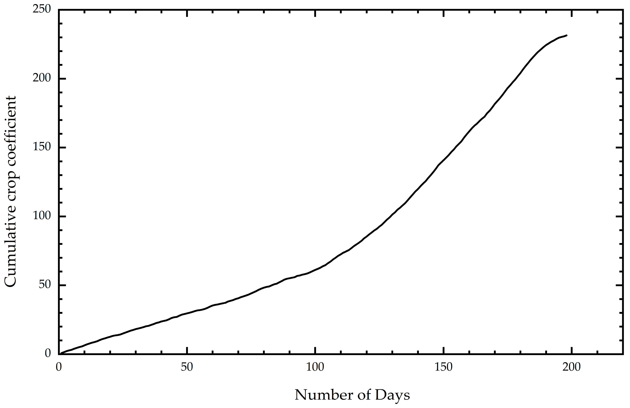
The curves of the cumulative crop coefficient and days after seeding of winter wheat are shown in Figure 2, showing an approximately elongated “S” shape. The daily growth value of the cumulative crop coefficient is that of the daily crop coefficient, which increases first and then decreases with time after seeding. The cumulative crop coefficient model was constructed as follows:
K c   cumulative = a + b × cos c × D + d × sin c × D
where Kc cumulative is the cumulative crop coefficient value, D is the number of days after seeding, and a, b, c, and d are unknown parameters.
For each growth stage, the least square method was used to estimate the values of unknown parameters a, b, c, and d. According to the definition of the function, its derivative is the daily value function of the crop coefficient, and the value of the crop coefficient on day D can be obtained by substituting D into it. The derivative of Equation (13) with respect to D can be obtained as follows:
K c = b × c × sin c × D + d × c × cos c × D

2.5.3. Radiative Soil Temperature Method

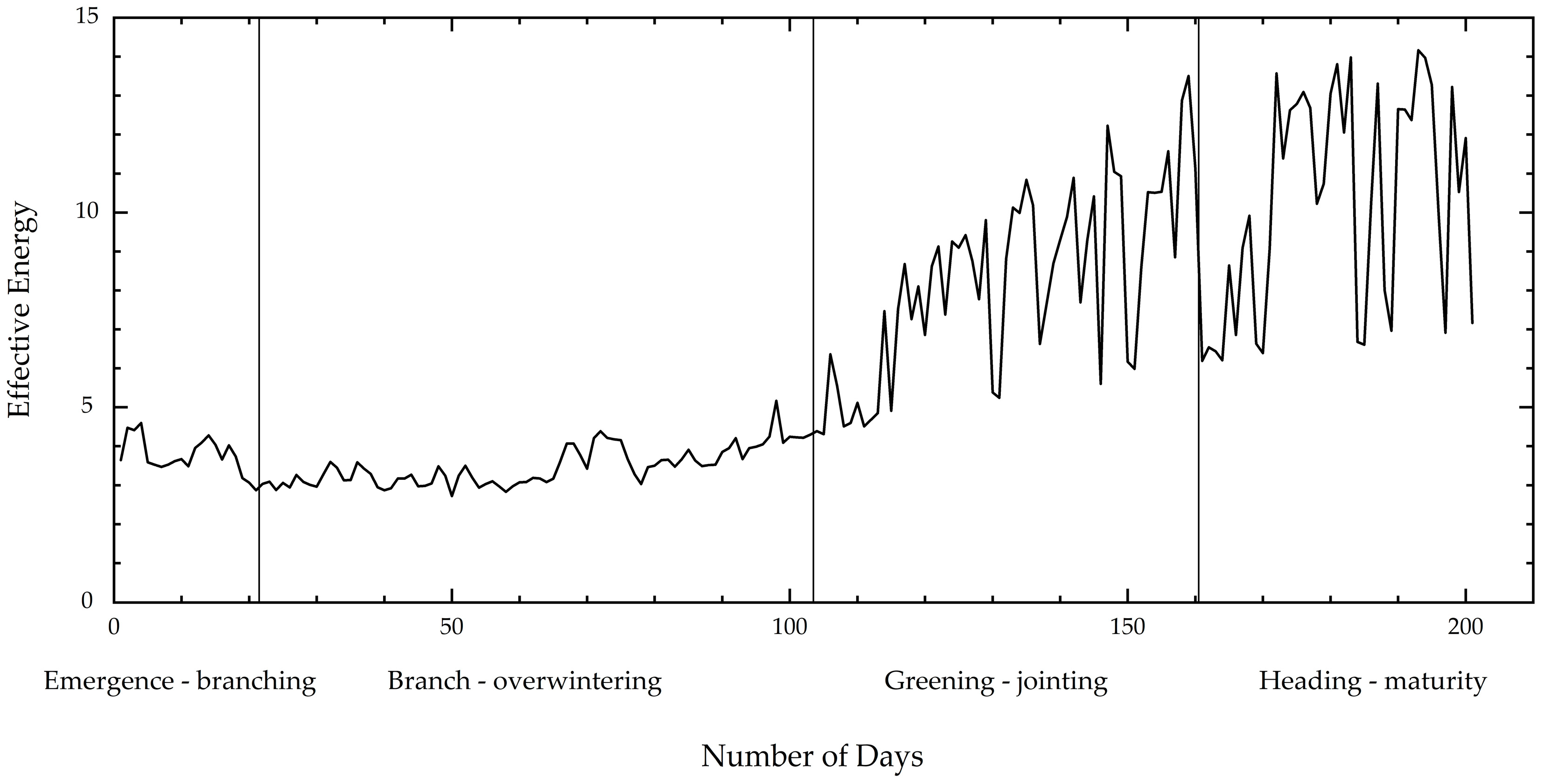
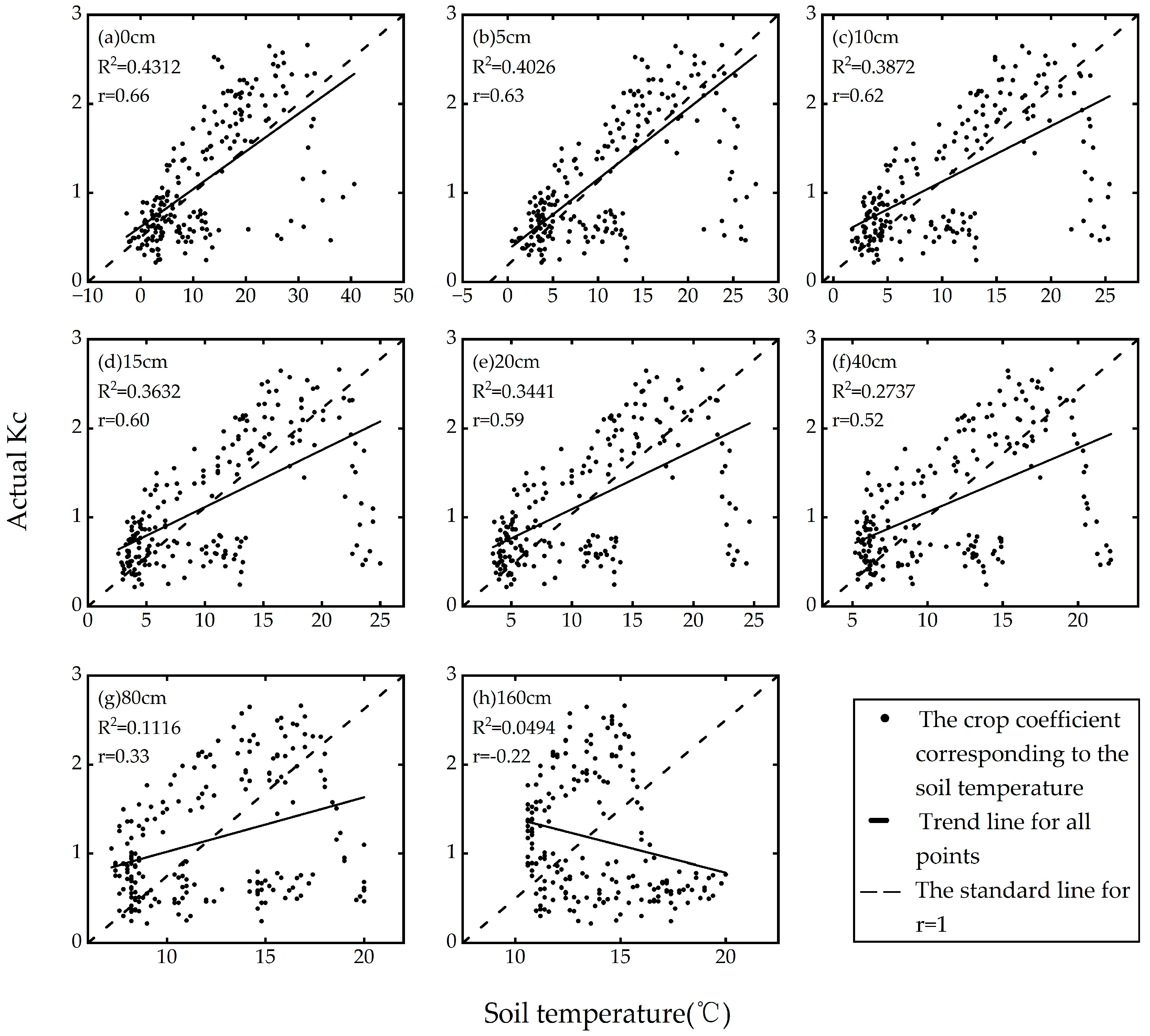
According to the study of Zhao et al. [31], there is a strong positive correlation between the crop coefficient and evapotranspiration and a significant positive correlation between evapotranspiration and effective energy. Effective energy (Rn-G) refers to the difference between net radiation and soil heat flux, showing a trend of being smaller at the emergence-branching and branch-overwintering stages and gradually increasing at the greening-jointing and heading-maturity stages (Figure 3). During the whole process of winter wheat growth, the correlation coefficient between the crop coefficient and effective energy reached 0.75, showing a strong correlation. The correlation coefficient between the crop coefficient and soil temperature from 0 to 160 cm decreased from 0.66 to 0.70 with increasing depth, as shown in Figure 4.
Because FAO-56 notes that the penetration depth of temperature waves in soil is 0.1 to 0.2 m at a daily scale, soil temperatures at 0 and 10 cm were selected. The following mathematical model was constructed involving radiation and soil temperature:
K c = me R n G n D 0 D 10
where D0 is the surface temperature (°C); D10 is the soil temperature of 10 cm (°C); and m and n are unknown parameters. The meanings of the other symbols are the same as described previously.
Parameter calibration was realized by the particle swarm optimization algorithm. After finding the unknown parameter values corresponding to the daily scale data of each group in the whole growth process, the best unknown parameter of each growth stage was obtained by taking the average value. The particle swarm optimization algorithm is a random optimization method based on swarm intelligence proposed by Kennedy and Eberhart [32]. Each particle represents a candidate solution, and the problem is solved through assessment of the simple behaviour of individual particles and information interaction within the group.
When solving the optimization problem, each particle has two state quantities, position and velocity, and the fitness value determined by the objective function. The flight process of the particle is the search process of the individual. In each iteration, individual particles record the best solution found as the current individual extreme value and share it with other particles. The best of all individual extreme values is the extreme value of the current group. All particles adjust their speed and position according to their current individual extreme value and the current group extreme value of the whole particle swarm [33]. Optimization was achieved using MATLAB software programming.
According to the properties of the model, in the two-dimensional solution search space, there is a particle swarm composed of 500 particles. The position of the particle swarm of the k-th iteration in the solution space is assumed to be expressed as Equation (16), and the flight velocity is expressed as Equation (17):
X i k = X i 1 k , X i 2 k , i = 1 , 2 , , 500
V i k = V i 1 k , V i 2 k , i = 1 , 2 , , 500
At this time, the best individual historical position of the jth (j < 500) particle is X mj 1 k , X mj 2 k , and the best historical position of the particle swarm is Y m 1 k , Y m 2 k . Then, at the k + 1 iteration, the velocity and position update formula of the particle is as follows:
V j 1 k + 1 = w × V j 1 k + c 1 × r 1 × X mj 1 k X j 1 k + c 2 × r 2 × Y m 1 k X j 1 k V j 2 k + 1 = w × V j 2 k + c 1 × r 1 × X mj 2 k X j 2 k + c 2 × r 2 × Y m 2 k X j 2 k
X i 1 k + 1 = X i 1 k + V j 1 k + 1 X i 2 k + 1 = X i 2 k + V j 2 k + 1
w = w min + w max w min × ger times ger
where w is the inertia weight, representing the influence of the current speed on the next movement; c 1 and c 2 are the learning factors, which measure the influence of the current individual historical optimal position and group historical optimal position on the next movement; r 1 and r 2 are random numbers from 0 to 1; w min is the initial inertia weight with a typical value of 0.4; w max is the inertia weight under the maximum number of iterations with a typical value of 0.9; ger is the maximum number of iterations; and times indicates the current iteration times.

2.5.4. Indices of Evaluation

The evaluation indices include the root mean square error (RMSE), mean absolute error (MAE), correlation coefficient (r), and consistency index (dIA), which are used to evaluate the error and consistency between the estimated value and the measured value of each estimation method. See Equation (21) to Equation (24) for the calculation formula of each index.
RMSE = i = 1 n x i y i 2 n
MAE = i = 1 n x i y i n
r = i = 1 n x i x ¯ y i y ¯ i = 1 n x i x ¯ 2 i = 1 n y i y ¯ 2
d IA = 1 i = 1 n x i y i 2 i = 1 n x i y ¯ + y i y ¯ 2
where x i is the estimated value of K c ; y i is the actual value of K c ; i is the sample ordinal number, i = 1 , 2 , , n ; x ¯ is the mean value of K c ’s estimation; y ¯ is the mean value of K c ; and n is the number of samples of the estimated value.
Generally, the closer the root mean square error RMSE and mean absolute error MAE are to 0, the smaller the error and the greater the accuracy. The closer the correlation coefficient r and the consistency index dIA are to 1, the closer the estimated value of the model is to the actual value, and the stronger its estimation ability is.

3. Results

Based on the observation data of the large weighing lysimeter and the data of the high-precision weather station from 2018 to 2019, the parameters of the three crop coefficient estimation models were calibrated. The unknown parameter values obtained by each method under different growth stages are shown in Table 2.

3.1. The Differences and Causes of Crop Coefficient Estimation by Different Methods

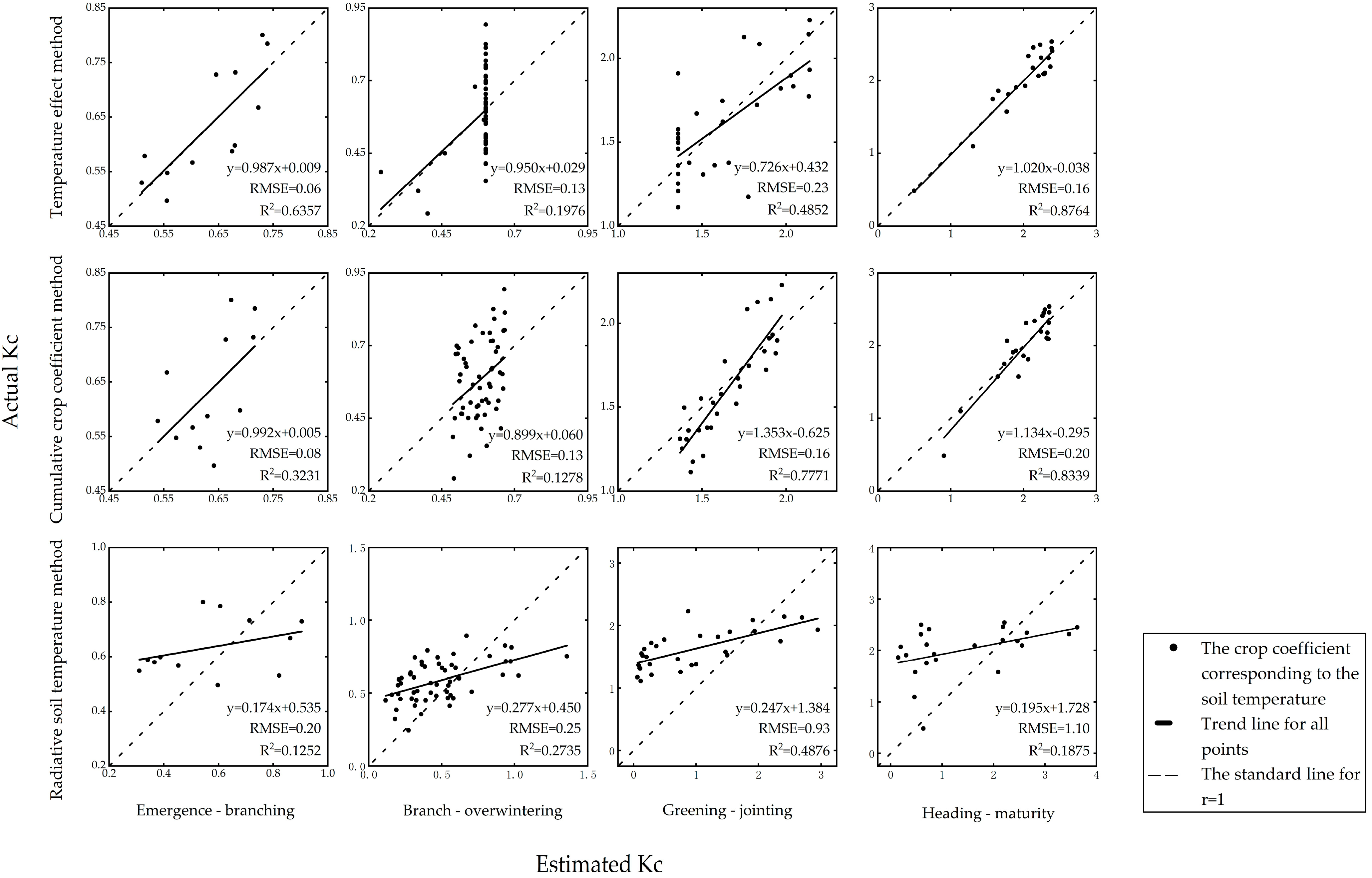
The results of the three methods for estimating winter wheat crop coefficients are shown in Figure 5 and Figure 6. The results of the temperature effect method were better in the emergence-branching and heading-maturity stages, followed by the greening-jointing and branch-overwintering stages. The reason was that there were fewer ineffective temperatures below 3 °C and above 30 °C during the emergence-branching and heading-maturity stages, and crop growth was not inhibited by ineffective temperatures. The cumulative crop coefficient method was better in the greening-jointing and heading-maturity stages but worse in the emergence-branching and branch-overwintering stages. The reason was that the cumulative crop coefficient method is closely related to crop growth [17], the leaf index in the greening-jointing and heading-maturity stages was larger [34,35], and crop growth and development were vigorous. The radiative soil temperature method was better in the emergence-branching and branch-overwintering stages but worse in the greening-jointing and heading-maturity stages. The reason was that the effective energy cannot maintain a high level during the greening-jointing and heading-maturity stages, and the balance between energy and soil temperature was difficult to ensure.

3.2. Determination of The Best Estimation Method for Each Growth Stage

The accuracy of the results of the three methods in each growth stage are shown in Table 3 (in this table, “TE” means the temperature effect method, “CCC” means the cumulative crop coefficient method, and “RST” means the radiative soil temperature method).
The estimation results were compared, and the best estimation method was selected according to the following steps. In the first step, the root mean square error, RMSE, and mean absolute error, MAE, were compared, and the method with the smallest error was selected. In the second step, when the difference in the root mean square error and mean absolute error between multiple methods are no more than 0.03, the correlation coefficient r and consistency index dIA are compared in turn to select the method with the strongest estimation ability. In the third step, if the difference between the correlation coefficient and consistency index is less than 0.03, then the cumulative crop coefficient method should be directly adopted according to the principle of minimum required observations if it is still in the option list. Otherwise, the most appropriate method should be adopted in combination with the graph.
According to the above criteria, the temperature effect method during the emergence-branching stage was the best (RMSE = 0.06, MAE = 0.06, r = 0.80, dIA = 0.88), followed by the cumulative crop coefficient method, and the radiative soil temperature method was inferior. The temperature effect method during the branch-overwintering stage was the best (RMSE = 0.13, MAE = 0.11, r = 0.44, dIA = 0.55), followed by the cumulative crop coefficient method, and the radiative soil temperature method was inferior. The cumulative crop coefficient method during the greening-jointing stage was the best (RMSE = 0.16, MAE = 0.13, r = 0.88, dIA = 0.89), followed by the temperature effect method, and the radiative soil temperature method was inferior. The temperature effect method during the heading-maturity stage was the best (RMSE = 0.16, MAE = 0.13, r = 0.94, dIA = 0.97), followed by the cumulative crop coefficient method, and the radiative soil temperature method was inferior.
The estimated accuracy index of the whole growth process when a single method or the best method is used in each growth stage is shown in Table 4. When a single method was used in each growth stage, the cumulative crop coefficient method was the best method for estimating the whole growth process (RMSE = 0.25, MAE = 0.20, r = 0.93, dIA = 0.96), followed by the temperature effect method, and the radiative soil temperature method was inferior. When the cumulative crop coefficient method and temperature effect method were used, the correlation coefficient and consistency index of the whole growth process estimation results were both greater than 0.80, which met the accuracy requirements of estimation and could be used for crop coefficient estimation. When the radiative soil temperature method was used, the correlation coefficient and consistency index of the whole growth process estimation results were only 0.50 and 0.69, respectively, which could not meet the requirement of estimation accuracy.
When the best method was used in each growth stage, the four precision indices were better than when a single method was used; the root mean square error and mean absolute error were 0.13 and 0.09, and the correlation coefficient and consistency index reached 0.98 and 0.99, far greater than 0.80. The best method has higher estimation ability and accuracy than the single method and can be used for crop coefficient estimation.

4. Conclusions and Discussion

1. The results of the temperature effect method were better in the emergence-branching and heading-maturity stages, followed by the greening-jointing and branch-overwintering stages. The reason was that the ineffective temperature was lower during the emergence-branching and heading-maturity stages, and crop growth was not inhibited. The cumulative crop coefficient method was better in the greening-jointing and heading-maturity stages but worse in the emergence-branching and branch-overwintering stages. The reason was that the cumulative crop coefficient method is closely related to crop growth, and the crops grew vigorously during the greening-jointing and heading-maturity stages. The radiative soil temperature method was better in the emergence-branching and branch-overwintering stages but worse in the greening-jointing and heading-maturity stages. The reason was that the effective energy could not maintain a high level during the greening-jointing and heading-maturity stages, and the energy balance was difficult to ensure.
2. The temperature effect method during the emergence-branching stage was the best, followed by the cumulative crop coefficient method, and the radiative soil temperature method was inferior. The temperature effect method during the branch-overwintering stage was the best, followed by the cumulative crop coefficient method, and the radiative soil temperature method was inferior. The cumulative crop coefficient method during the greening-jointing stage was the best, followed by the temperature effect method, and the radiative soil temperature method was inferior. The temperature effect method during the heading-maturity stage was the best, followed by the cumulative crop coefficient method, and the radiative soil temperature method was inferior.
3. When a single method was used in each growth stage, the cumulative crop coefficient method was the best, followed by the temperature effect method, and the radiative soil temperature method was inferior. The cumulative crop coefficient method and temperature effect method meet the accuracy requirements of estimation, but the radiative soil temperature method could not meet the accuracy requirements of estimation. The root mean square error, RMSE = 0.13; mean absolute error, MAE = 0.09; correlation coefficient, r = 0.98; and consistency index, dIA = 0.99 were all better than the single method when the best method was used in each growth stage. The best method had higher estimation ability and accuracy than the single method.
To improve upon the results presented in this paper, the adaptability of different crop coefficient estimation methods in other areas needs to be further explored. In addition, the daily crop coefficient estimation is only discussed under the condition of 1 m burial depth. The difference in the estimation effect of different methods under different burial depths needs to be further studied. In addition to crop growth traits, there is also the standard crop coefficient stage division table recommended by the FAO. Different division methods also have a certain impact on the accuracy of estimation. In the future, more crop coefficient estimation methods can be considered to provide more options for crop coefficient estimation.

Author Contributions

Conceptualization, J.F.; Formal analysis, J.F.; Investigation, J.F.; Resources, C.Z.; Data curation, C.Z., Y.L., P.G. and B.S.; Writing – original draft, J.F.; Writing – review & editing, Y.W., P.J. and Q.J.; Visualization, Y.L., P.G. and B.S.; Funding acquisition, Y.W. All authors have read and agreed to the published version of the manuscript.

Funding

This work was supported by the Youth Fund of National Natural Science Foundation of China (Grant No. 52109029), the National key research and development program funded project of China (Grant No. 2022YFC3202401), the Belt and Road Special Foundation of the State Key Laboratory of Hydrology-Water Resources and Hydraulic Engineering (Grant No. 2020490211; Grant No. 2020490208), the Water science and technology project of Jiangsu Province (Grant No. 2021047), the Independent research project of State Key Laboratory of Hydrology, Water Resources and Hydraulic Engineering (Grant No. 522012222), and the Basic research projects of central level public welfare research institutes (Grant No. Y522003).

Data Availability Statement

No new data were created or analyzed in this study. Data sharing is not applicable to this article.

Conflicts of Interest

The authors declare no conflict of interest.

Abbreviations

The following abbreviations are used in this manuscript:
FAOFood and Agriculture Organization
FAO-56FAO Irrigation and Drainage Paper No. 56
KcCrop coefficient
ETActual evapotranspiration
KsWater stress coefficient
TCARITransformed chlorophyll absorption in reflectance index
RDVIRenormalized difference vegetation index
UAVUnmanned aerial vehicle
TSEBTwo-source energy balance
ET0Reference evapotranspiration
SPSSStatistical Product and Service Solutions
Rn-GEffective energy
MATLABMatrix Laboratory
rCorrelation coefficient
dIAConsistency index
RMSERoot mean square error
MAEMean absolute error
TETemperature effect method
CCCCumulative crop coefficient method
RSTRadiative soil temperature method

References

  1. Daszkiewicz, T. Food Production in the Context of Global Developmental Challenges. Agriculture 2022, 12, 832. [Google Scholar] [CrossRef]
  2. Wu, B.F.; Tian, F.Y.; Zhang, M.; Piao, S.L.; Zeng, H.W.; Zhu, W.W.; Liu, J.G.; Elnashar, A.; Lu, Y.M. Quantifying global agricultural water appropriation with data derived from earth observations. J. Clean. Prod. 2022, 358, 131891. [Google Scholar] [CrossRef]
  3. Kabbadj, A.; Makoudi, B.; Mouradi, M.; Pauly, N.; Frendo, P.; Ghoulam, C. Physiological and biochemical responses involved in water deficit tolerance of nitrogen-fixing vicia faba. PLoS ONE 2017, 12, e0190284. [Google Scholar] [CrossRef] [PubMed] [Green Version]
  4. Paul, A.S.; Panwar, N.L.; Salvi, B.L.; Jain, S.; Sharma, D. Experimental investigation on the production of bio-oil from wheat straw. Energy Sources Part A Recovery Util. Environ. Eff. 2020, 6, 1–16. [Google Scholar] [CrossRef]
  5. Langridge, P.; Alaux, M.; Almeida, N.F.; Ammar, K.; Baum, M.; Bekkaoui, F.; Bentley, A.R.; Beres, B.L.; Berger, B.; Braun, H.J.; et al. Meeting the Challenges Facing Wheat Production: The Strategic Research Agenda of the Global Wheat Initiative. Agronomy 2022, 12, 2767. [Google Scholar] [CrossRef]
  6. Xiang, C.; Huang, J.K. The role of exotic wheat germplasms in wheat breeding and their impact on wheat yield and production in china. China Econ. Rev. 2020, 62, 101239. [Google Scholar] [CrossRef]
  7. Dong, J.; Fu, Y.Y.; Wang, J.J.; Tian, H.F.; Fu, S.; Niu, Z.; Han, W.; Zheng, Y.; Huang, J.X.; Yuan, W.P. Early-season mapping of winter wheat in china based on landsat and sentinel images. Earth Syst. Sci. Data 2020, 12, 3081–3095. [Google Scholar] [CrossRef]
  8. Park, J.; Baik, J.; Choi, M. Satellite-based crop coefficient and evapotranspiration using surface soil moisture and vegetation indices in northeast asia. Catena 2017, 156, 305–314. [Google Scholar] [CrossRef]
  9. Shan, N.; Zhang, Y.G.; Cheng, J.M.; Ju, W.M.; Migliavacca, M.; Penuelas, J.; Yang, X.; Zhang, Z.Y.; Nelson, J.A.; Goulas, Y. A model for estimating transpiration from remotely sensed solar-induced chlorophyll fluorescence. Remote Sens. Environ. 2021, 252, 112–134. [Google Scholar] [CrossRef]
  10. Allen, R.G.; Pereira, L.S.; Raes, D.; Smith, M. Crop Evapotranspiration-Guidelines for Computing Crop Water Requirements-FAO Irrigation and Drainage Paper 56; FAO: Rome, Italy, 2008.
  11. Er-Raki, S.; Chehbouni, A.; Guemouria, N.; Duchemin, B.; Ezzahar, J.; Hadria, R. Combining fao-56 model and ground-based remote sensing to estimate water consumptions of wheat crops in a semi-arid region. Agric. Water Manag. 2007, 87, 41–54. [Google Scholar] [CrossRef] [Green Version]
  12. Vu, S.H.; Watanabe, H.; Takagi, K. Application of fao-56 for evaluating evapotranspiration in simulation of pollutant runoff from paddy rice field in japan. Agric. Water Manag. 2005, 76, 195–210. [Google Scholar] [CrossRef]
  13. Mokhtari, A.; Noory, H.; Vazifedoust, M.; Bahrami, M. Estimating net irrigation requirement of winter wheat using model- and satellite-based single and basal crop coefficients. Agric. Water Manag. 2018, 208, 95–106. [Google Scholar] [CrossRef]
  14. Spiliotopoulos, M.; Loukas, A. Hybrid Methodology for the Estimation of Crop Coefficients Based on Satellite Imagery and Ground-Based Measurements. Water 2019, 11, 1364. [Google Scholar] [CrossRef] [Green Version]
  15. Zhang, Y.; Han, W.T.; Niu, X.T.; Li, G. Maize Crop Coefficient Estimated from UAV-Measured Multispectral Vegetation Indices. Sensors 2019, 19, 5250. [Google Scholar] [CrossRef] [PubMed] [Green Version]
  16. Wang, Z.L.; Gu, N.; Lu, H.S.; Hu, Y.S.; Zhu, Y.H.; Yang, M. Calculation method of crop coefficient and evapotranspiration basedon temperature effect. J. Hydraul. Eng. 2019, 50, 242–251. [Google Scholar]
  17. Tang, J.D. Estimation Method of Maize Water Use Efficiency and Biomass Based on UAV Remote Sensing. Master’s Thesis, Northwest A F University, Xianyang, China, 2021. [Google Scholar]
  18. Kool, D.; Kustas, W.P.; Ben-Gal, A.; Agam, N. Energy partitioning between plant canopy and soil, performance of the two-source energy balance model in a vineyard. Agric. For. Meteorol. 2021, 300, 108328. [Google Scholar] [CrossRef]
  19. Paulino, S.E.P.; Mourao, F.D.A.; Maia, A.D.N.; Aviles, T.E.C.; Neto, D.D. Agrometeorological models for ‘valencia’ and ‘hamlin’ sweet oranges to estimate the number of fruits per plant. Sci. Agric. 2007, 64, 1–11. [Google Scholar] [CrossRef] [Green Version]
  20. Ju, Q.; Liu, X.N.; Liu, Z.T.; Gao, H.B.; Zhao, W.J.; Nimazhaxi; Hao, W.L. Response and prediction of groundwater depth change to climate change in Huaibei Plain. Trans. Chin. Soc. Agric. Eng. 2022, 38, 136–145. [Google Scholar]
  21. Zhu, Y.H.; Ren, L.L.; Horton, R.; Lu, H.S.; Wang, Z.L.; Yuan, F. Estimating the Contribution of Groundwater to the Root Zone of Winter Wheat Using Root Density Distribution Functions. Vadose Zone J. 2018, 17, 1–15. [Google Scholar] [CrossRef] [Green Version]
  22. Xu, J.Z.; Peng, S.Z.; Ding, J.L.; Wei, Q.; Yu, Y.M. Evaluation and calibration of simple methods for daily reference evapotranspiration estimation in humid East China. Arch. Agron. Soil Sci. 2013, 59, 845–858. [Google Scholar] [CrossRef]
  23. Huang, C.P.; Zhang, F.; Wang, A.H.; Hu, B.M.; Yang, J.H. Dynamic simulation of potato growth process. J. Appl. Ecol. 2004, 15, 1203–1206. [Google Scholar]
  24. Qureshi, Z.A.; Neibling, H. Response of two-row malting spring barley to water cutoff under sprinkler irrigation. Agric. Water Manag. 2009, 96, 141–148. [Google Scholar] [CrossRef]
  25. Rosa, H.T.; Walter, L.C.; Streck, N.A.; Alberto, C.M. Thermal time methods and sowing dates in phyllochron determination in wheat cultivars. Pesqui. Agropecuária Bras. 2009, 44, 1374–1382. [Google Scholar] [CrossRef]
  26. Wechsung, F.; Ritter, M.; Wall, G.W. The upper homeostatic range for the temperature–yield response of irrigated us wheat down revised from a theoretical and experimental perspective. Agric. For. Meteorol. 2021, 307, 108478. [Google Scholar] [CrossRef]
  27. Porter, J.R.; Gawith, M. Temperatures and the growth and development of wheat: A review. Eur. J. Agron. 1999, 10, 23–36. [Google Scholar] [CrossRef]
  28. Qi, S.H.; Wang, B.J.; Wu, Z.S. The relationship between agricultural production and temperature. J. Henan Inst. Sci. Technol. (Nat. Sci. Ed.) 2007, 35, 20–23. [Google Scholar]
  29. Su, L.J.; Wang, Q.J.; Bai, Y.G. An analysis of yearly trends in growing degree days and the relationship between growing degree day values and reference evapotranspiration in Turpan area, China. Theor. Appl. Climatol. 2013, 113, 711–724. [Google Scholar] [CrossRef]
  30. Lewis, C.S.; Allen, L.N. Potential crop evapotranspiration and surface evaporation estimates via a gridded weather forcing dataset. J. Hydrol. 2017, 546, 450–463. [Google Scholar] [CrossRef] [Green Version]
  31. Zhao, Y.; Mao, X.M.; Shukla, M.K.; Tian, F.; Hou, M.J.; Zhang, T.; Li, S.E. How does film mulching modify available energy, evapotranspiration, and crop coefficient during the seed–maize growing season in northwest china? Agric. Water Manag. 2021, 245, 106666. [Google Scholar] [CrossRef]
  32. Weerasinghe, G.; Chi, H.M.; Cao, Y.Z. Particle Swarm Optimization Simulation via Optimal Halton Sequences. Procedia Comput. Sci. 2016, 80, 772–781. [Google Scholar] [CrossRef] [Green Version]
  33. Benuwa, B.B.; Ghansah, B.; Wornyo, D.K.; Adabunu, S.A. A Comprehensive Review of Particle Swarm Optimization. Int. J. Eng. Res. Afr. 2016, 23, 141–161. [Google Scholar] [CrossRef]
  34. Du, X.B.; Wang, Z.; Xi, M.; Wu, W.G.; Wei, Z.; Xu, Y.Z.; Zhou, Y.J.; Lei, W.X.; Kong, L.C. A novel planting pattern increases the grain yield of wheat after rice cultivation by improving radiation resource utilization. Agric. For. Meteorol. 2021, 310, 108625. [Google Scholar] [CrossRef]
  35. Li, Y.X.; Liu, H.J.; Ma, J.C.; Zhang, L.X. Estimation of leaf area index for winter wheat at early stages based on convolutional neural networks. Comput. Electron. Agric. 2021, 190, 106480. [Google Scholar] [CrossRef]
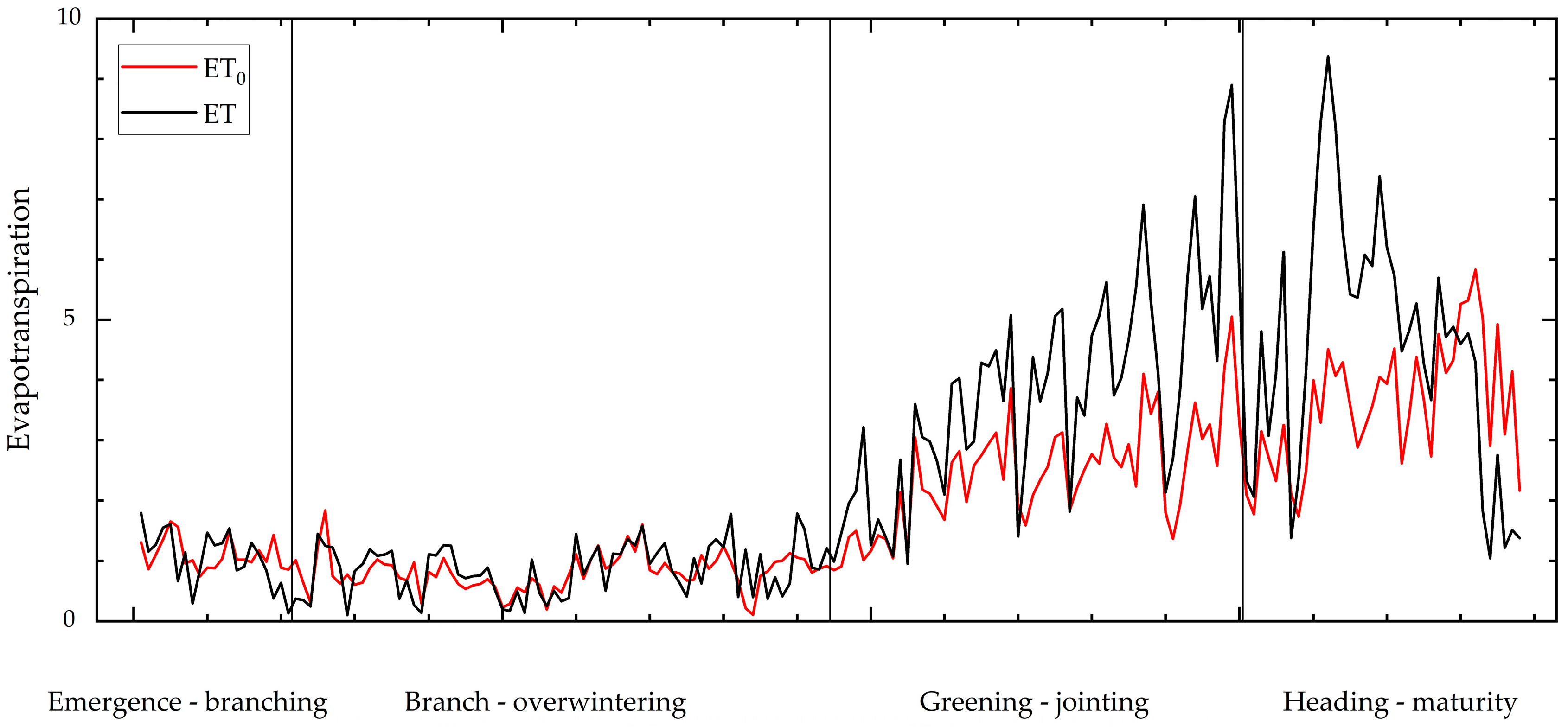
Figure 1. The variation of the actual evapotranspiration (ET) and reference evapotranspiration (ET0).
Water 15 01395 g001
Figure 2. Correlation curve between cumulative crop coefficient and days after seeding.
Water 15 01395 g002
Figure 3. The variation of the effective energy (Rn-G).
Water 15 01395 g003
Figure 4. Correlation between crop coefficient and soil temperature from 0 to 160 cm(a to h in the figure represent the deepening of soil depth).
Water 15 01395 g004
Figure 5. Results of three methods for estimating winter wheat crop coefficients.
Water 15 01395 g005
Figure 6. The estimated crop coefficient and actual crop coefficient during four growing stages.
Water 15 01395 g006
Table 1. Growth stage division of winter wheat.
Stage of GrowthEmergence-Branching Branch-Overwintering Greening-Jointing Heading-Maturity
Date2018/11/11–2018/12/12018/12/2–2019/2/212019/2/22–2019/4/192019/4/20–2019/6/4
Number of days21825746
ET0 at this stage21.80 mm67.80 mm216.48 mm220.67 mm
Proportion of total ET04.14%12.87%41.10%41.89%
Average daily ET01.04 mm0.83 mm3.80 mm4.80 mm
Table 2. Values of unknown parameters in different growth stages and methods of winter wheat.
MethodTemperature EffectCumulative Crop CoefficientRadiative Soil Temperature
Parameter K 0 T 0 β a b c d m n
Emergence-branching stage1.243.0018.84158.62−7.170.076.544.195.87
Branch-overwintering stage1.963.0012.42216.22−79.900.0160.000.263.21
Greening-jointing stage2.1420.956.61180.23−382.33−0.0126.250.415.62
Heading-maturity stage2.3920.375.16227.910.02−0.0543.526.168.81
Table 3. The estimated precision index value of the results of three methods in each growth stage.
StageEmergence-Branching StageBranch-Overwintering StageGreening-Jointing StageHeading-Maturity Stage
IndexRMSEMAErdIARMSEMAErdIARMSEMAErdIARMSEMAErdIA
TE0.060.060.800.880.130.110.440.550.230.180.700.830.160.130.940.97
CCC0.080.070.570.690.130.120.360.510.160.130.880.890.200.160.910.94
RST0.200.190.350.510.250.220.520.610.930.790.700.491.100.910.430.49
Table 4. The estimation precision index values of the whole growth process.
MethodRoot Mean Square ErrorMean Absolute ErrorCorrelation CoefficientConsistency Index
TE0.340.250.870.93
CCC0.250.200.930.96
RST0.790.580.500.69
The best0.130.090.980.99
Disclaimer/Publisher’s Note: The statements, opinions and data contained in all publications are solely those of the individual author(s) and contributor(s) and not of MDPI and/or the editor(s). MDPI and/or the editor(s) disclaim responsibility for any injury to people or property resulting from any ideas, methods, instructions or products referred to in the content.