Abstract
Rapid prediction of urban flooding is an important measure to reduce the risk of flooding and to protect people’s property. In order to meet the needs of emergency flood control, this paper constructs a rapid urban flood prediction model based on a machine learning approach. Using the simulation results of the hydrodynamic model as the data driver, a neural network structure combining convolutional neural network (CNN) and long and short-term memory network (LSTM) is constructed, taking into account rainfall factors, geographical data, and the distribution of the drainage network. The study was carried out with the central city of Zhoukou as an example. The results show that after the training of the hydrodynamic model and CNN−LSTM neural network model, it can quickly predict the depth of urban flooding in less than 10 s, and the average error between the predicted depth of flooding and the measured depth of flooding does not exceed 6.50%, which shows that the prediction performance of the neural network is good and can meet the seeking of urban emergency flood control and effectively reduce the loss of life and property.
1. Introduction
Against the backdrop of frequent global weather extremes and accelerated urbanization, extreme precipitation is increasing and intensifying [1], and waterlogging caused by rainfall is becoming a “normalized” risk. In recent years, there have been a number of major disasters caused by heavy rainfall. On 21 July 2012, an extremely heavy rainfall in Beijing caused the collapse of 10,600 houses and affected 1.9 million people [2]. On 11 April 2019, a short period of extreme precipitation caused some areas in Shenzhen to be flooded and 11 people drowned [3]. On 21 July 2021, the heavy rainfall in Zhengzhou caused 14,786,000 people to be affected and 398 people to die or go missing [4]. Rapid prediction and warning of urban flooding caused by heavy rainfall is an effective way to improve the ability of government departments to deal with disasters.
At present, scholars have conducted a lot of research on the prediction of storm water flooding. The commonly used hydrodynamic models for predicting urban flooding mainly include the Storm Water Flood Management Model (SWMM), the Integrated Urban Watershed Drainage Model (infoWorks ICM), MIKE URBAN, etc. These models calculate the water flow state by solving hydrodynamic equations, with clear physical mechanisms and easy to obtain high precision numerical simulations results. For example, Li et al. [5] used the Minzhi area of Shenzhen City as the research object and constructed a rainfall model based on a 1D and 2D coupled urban flooding numerical model to simulate the flooding situation in the area, and used ArcGIS and hierarchical analysis to evaluate the flooding hazard in the area. Harsha et al. [6] used a densely populated area in Vijayawada, India, to simulate the surface runoff and network water volume data under extreme rainfall events. Zhang et al. [7] used a pilot sponge city area in Ningbo to simulate the flooding risk under short and long recurrence periods of design rainfall. Sarkar et al. [8] used four areas in Khulna, Bangladesh, to simulate and analyze the surface runoff, inundation level, drainage capacity, and the impact of urban flooding on municipal traffic and buildings based on the MIKE model. Li et al. [9] used the Huangtaiqiao watershed in Jinan City as the research object, coupled the SWMM 1D pipe network model with the LISTLOOD FP 2D surface inundation model, and analyzed the number of overflow nodes and their spatial distribution characteristics under different recurrence period design precipitation. Ren et al. [10] used the Dongtang Wei area of Chaohu City as a research object to construct a fully distributed refined urban flooding model and compared its simulation differences with the traditional SWMM model under different storm scenarios. However, the numerical model is complex and time-consuming to solve under large scale and complex subsurface conditions, and it is difficult to meet the time-effective requirements of storm water prediction.
In recent years, to make up for the shortcomings of numerical models, scholars have gradually applied machine learning methods to storm water flooding disaster prediction. Kan et al. [11] coupled ANN with K-neighborhood methods to improve problems such as a poor ANN forecasting ability. Liu et al. [12] proposed a new method for predicting urban flooding risk based on the combination of BP neural networks and numerical models. Mei et al. [13] conducted flood forecasting based on support vector machines, and the model had the advantages of a strong generalization ability and fast training speed. Hou et al. [14] considered meteorological, geographical, and social factors and used a neural network model to achieve a short-time prediction calculation of the depth of water accumulation at a single point. Li et al. [15] constructed a storm flooding disaster prediction model and found that the XGBoost model performed better than a back propagation neural network. These studies show that machine learning techniques also have broad application prospects in urban flooding prediction.
In this paper, high-precision data obtained from numerical simulations are used as the data set. A neural network structure combining convolutional neural network (CNN) and long short-term memory network (LSTM) is constructed. The data set from the numerical simulation is used for learning and training to achieve rapid prediction of waterlogging depth, which can provide scientific reference for early warning and forecasting of urban flooding, as well as disaster prevention and mitigation work.
2. Materials and Methods
2.1. Research Process
In the study of urban flooding prediction, efficient simulation of the urban flooding process can often improve the accuracy of rainfall forecast data [16]. In this paper, based on the hydrodynamic model and machine learning algorithm (CNN−LSTM), a numerical model is established to simulate the 3 h short calendar time intense rainfall process in the central city of Zhoukou as a rainfall scenario, and the simulation results are used as the data driver for neural network prediction at each waterlogged point. The process is shown in Figure 1.
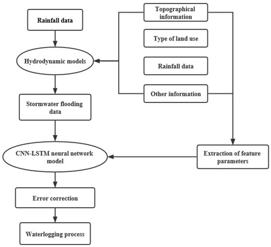
Figure 1.
Technical flow chart.
The data-driven model for predicting the depth of water in urban storms consists of two main components.
- (1)
- Generating time series data on flooding
Urban storm waterlogging data are typically time series data, and the urban storm waterlogging prediction problem is also a unique time series prediction problem, i.e., the data at one moment has a large impact on the data at a later moment, and thus can be converted into a supervised learning problem. Assuming that the current moment is t, the first three time steps, i.e., moment t − 3, moment t − 2, moment t − 1, are entered to predict the water depth values for the next two time steps, i.e., moment t, moment t + 1. The flooding features extracted from the rainfall, etc., data are first taken, followed by time-series-based prediction and specific methods such as data normalization, reconstruction to supervised data, and data complementary length to generate urban storm flooding time series data as a direct input to the subsequent bathymetric prediction model.
Supervised learning refers to the process of learning a mapping function relationship between the input to output using an algorithm oriented to the input variable X and the output variable Y. The expression is as follows.
Y = f(x)
It is called supervised learning because the data input to the model are labelled and the algorithm iterates continuously to achieve predictions on the training data, updating and correcting the model parameters by comparing the differences between the predicted labels and the true labels, and stopping learning when the performance of the algorithm reaches an acceptable level.
- (2)
- Building a neural network structure
A neural network structure combining CNN and LSTM was developed to predict urban storm flooding with multivariate inputs and multiple time steps. The neural network structure combines CNN and LSTM deep learning algorithms, using CNN to extract the spatial features of flooding, and then LSTM to extract the temporal features of flooding, and finally output the depth of urban storm flooding predicted by the model.
2.2. Hydrodynamic Models
The MIKE URBAN model simulates urban drainage networks into two broad steps: firstly, rainfall runoff simulation, based on the division of the corresponding catchment area through urban rainwater wells, and inputting rainfall boundary conditions to simulate a series of urban surface catchment processes such as rainfall, flow production, and confluence. The main hydrological models used to simulate this process are the time−area curve model, the non-linear reservoir model, the linear reservoir model, and the unit hydrological process line model. The most commonly used model for practical calculations is the time−area curve model, which is divided into two modules: production flow control and confluence control. The parameters to be determined for production flow control are impermeability, initial loss, and subsequent loss (hydrological attenuation coefficient), while the parameters to be determined for confluence control are time−area curve type and confluence time (average flow rate).
This is followed by the pipe network simulation, where the input boundary conditions are the flow process lines output from the previous step of the rainfall runoff simulation. Traditional network hydraulic calculations assume a constant flow in the pipe and use the inferential equation method, the results of which do not accurately interpret the actual flow process in the pipe. In contrast, the MIKE URBAN model uses non-constant flow in the hydraulic calculation of the pipe network, and applies the implicit finite difference method to solve the system of St. Venant equations for 1D free surface flow [17], and the simulation results are more accurate.
2.3. Combined CNN and LSTM Neural Network Structures
Urban storm water depth prediction is a multivariate input multiple time step output time series prediction problem. In this paper, the input data features are rainfall, water depth, time, slope, pipe network density, road network density, water system density, and land use type for the first three moments. The output data features are the predicted water depths at the last two moments. In this paper, a combined CNN and LSTM deep learning neural network is constructed by combining the input data features and the output data features. The CNN layer is responsible for extracting the spatial features of the input data for internal flooding. The CNN layer is responsible for extracting the spatial features of the input data, while the LSTM layer is responsible for acquiring the temporal features of flooding by taking a single rainfall event as a whole. In this paper, the depth of the neural network is increased to improve the ability of the model to predict the depth of urban storm waterlogging. The neural network structure of the combined CNN and LSTM is shown in Figure 2.

Figure 2.
Structure of the neural network combining CNN and LSTM.
The study of urban storm water depth prediction needs to take into account the ability of the model to represent both temporal and spatial features. Therefore, this paper proposes a deep learning neural network structure combining CNN and LSTM, taking into account the complementary nature of CNN and LSTM when constructing the urban storm water depth prediction model. CNN is used to capture the spatial characteristics and local variations of urban storm waterlogging temporal data, and LSTM is used to learn the short-time variation characteristics and long-time period characteristics of urban storm waterlogging temporal data, so as to improve the performance of the data-driven urban storm waterlogging prediction model and make it better able to simulate and forecast urban storm waterlogging characteristics.
2.4. Convolutional Neural Networks (CNN)
CNN was proposed by LeCun [18] and others, and is able to discard useless information, reduce network parameters, and speed up model training. Its implicit layer is mainly composed of three parts: convolutional layer, pooling layer, and fully connected layer. CNNs are suitable for studying the extended domain of spatial features of data, and are distinguished by their local connectivity and parameter sharing, and are often used to extract local variations in data, which can then be abstracted and combined into higher-level effective features.
In the data-driven urban storm water depth prediction model of this paper, the input data features are set as rainfall, water depth, time, slope, pipe network density, road network density, water system density, and land use type for the first three moments and the output data features are the predicted water depth for the last two moments. The convolution layer in CNN is first used to process and extract the values of the main geographical feature factors in the input data, by setting an M × N matrix as the convolution kernel and sliding over the whole input feature matrix according to a certain step size; each time the convolution kernel is moved, the dot product operation is repeated to obtain the corresponding local matrix [19]. This convolution process retains the original order of the input factors, discards some features, and reduces the number of weight parameters, thus reducing the computational pressure of the neural network; then, the pooling layer in CNN is used to sample the output of the previous convolution, which reduces the spatial dimension of the vectors in the model while ensuring that the depth of the network remains unchanged. This reduces the spatial dimension of the vectors in the model, and reduces the number of parameters and data features in the hidden layer to reduce the computational complexity of the model.
2.5. LSTM Neural Network Model
LSTM solves the problem of gradient disappearance and gradient explosion during the training of long sequences [20]. Its hidden layer consists of one or more memory units that are responsible for remembering arbitrary time intervals, and each memory unit has three “gate” structures, i.e., forgetting, input, and output gates. The so-called “gate” is a sigmod activation function applied to each matrix element and calculated by multiplying the corresponding elements. The memory cell structure of LSTM is shown schematically in Figure 3.
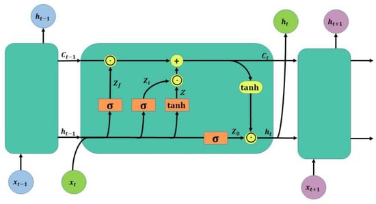
Figure 3.
Structure of LSTM.
In Figure 2, the input urban storm flooding time series data is x, the current moment is t, h is the output of a single LSTM memory cell, and σ denotes the chosen activation function, e.g., the sigmoid function. Zf, Zi, and Z0 are converted from the splicing vector multiplied by the weight matrix and then converted to a value between 0 and 1 by the activation function sigmoid as a gating state. In this paper, we increase the depth of the LSTM to better implement the learning of short-time variation features and long-time periodic features of urban storm water depth, which is implemented as follows.
In this paper, a data-driven model for predicting the depth of urban storm water flooding first uses the forgetting gate in the LSTM neural unit to selectively lose some information. This is done by using the current input urban storm flooding time series data Xt and the flooding time series output data ht−1 of the previous memory unit to generate a scale value between 0 and 1, which is used to determine the probability of information forgetting in the previous long-term state; when the value is equal to 0, all information is lost, and when the value is 1, the complete information is preserved. Next, the input gate in LSTM is used to add information, and when the input urban storm waterlogging time series data Xt and the output data ht−1 of the previous memory unit at this moment pass through the input gate, the information to be updated is determined and the new candidate memory unit is obtained through the tanh layer; then the output gate in LSTM is obtained and the previous long-term state is updated to the final state by the joint action of the forgetting gate and the input gate. Finally, the hidden state activated in the previous step is combined with the urban storm flooding time series data input at the current moment to update the hidden state, and multiplied with the hidden state activated in the tanh layer to obtain the final state output which is the final predicted water depth of the model.
2.6. Predictive Model Accuracy Validation
2.6.1. Cross-Validation Methods
In order to validate the simulation performance of the data-driven urban storm water depth prediction model in this paper on new sample data, it is usually necessary to divide the experimental data into training and test sets in advance. Considering the instability of the prediction results obtained from a single data division, and at the same time, in order to try to avoid the influence of subjective factors caused by the artificial allocation of data sets, this paper will combine the cross-validation approach to reduce the chance in order to compensate for the lack of accuracy of the experimental data and to improve the prediction accuracy of the model as much as possible. In this experiment, the ten-fold cross-validation method [21] is used to analyze the model prediction results and to test the accuracy and validity of the data-driven urban storm water depth prediction model in this paper. In this paper, the ten-fold cross-validation method is applied: firstly, the urban storm waterlogging time series data samples are randomly partitioned into ten, then nine of them are randomly selected as the training set for learning and training, and the last one is used as the model test set for validation. The accuracy and reliability of the CNN−LSTM-based urban storm water depth prediction results can be tested and guaranteed. The mean squared error (MSE) is within 0.03 after ten-fold cross-validation. The mean absolute error (MAE) is within 0.06 on average.
2.6.2. Model Evaluation Methods
In order to evaluate and validate the accuracy of the CNN−LSTM-based urban storm water depth prediction results, it is also necessary to introduce uniform evaluation metrics. In this paper, the mean square error (MSE), mean absolute error (MAE), and goodness of fit (R2) metrics are mainly used for determination.
Mean square error (MSE), the loss function of the model, is often used as an evaluation indicator for neural network regression models. A smaller value indicates that the error between the prediction result of this model and the true observation is smaller. The formula for calculating this value is as follows.
The mean absolute error (MAE) is the average of the absolute errors, which can better reflect the mean absolute deviation between the predicted bathymetric values of the model and the true observed values; a smaller value indicates that the error between the prediction results of the model in this paper and the true observed values is smaller. The value is calculated as follows.
The goodness of fit is often used to assess how well the model is fit, i.e., how well the model can explain the proportion of the variation in the dependent variable through the independent variables. The range of values is [0, 1]: if the value is 0, the model is a poor fit; if the result is 1, the model is error-free. The larger the value of the goodness of fit, the better the model fit. The formula for calculating this value is expressed as follows.
3. Results and Discussion
3.1. Hydrodynamic Model Validation and Training Sample Generation
Using the period of 20 July 2021 in Zhoukou City as an example to illustrate, 20 major waterlogging points in the central city were selected and the distribution of waterlogging points is shown in Figure 4. The measured maximum ponding depth data were compared with the maximum ponding depth simulated by the numerical model, as shown in Table 1. It can be seen that the simulated and measured values were close to each other, and the difference was within 5 cm, which was a small error, indicating that the numerical model was close to reality and qualitatively met the requirements of neural network learning. The inundation sample data obtained from the hydrodynamic model were used to build separate neural network models for each of the 20 major waterlogging points.
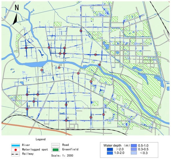
Figure 4.
Distribution of major waterlogged sites for 20 July 2021.

Table 1.
Comparison of measured and numerically modelled ponding depths at inundated water points for 20 July 2021.
The rainfall scenarios included actual short duration historical heavy rainfall processes from 1975–2019 and design rainfall based on the Zhoukou City storm intensity formula. A total of 832 rainfall scenarios with a duration of 3 h were calculated, and 20,422 storm inundation samples were obtained. The number and type of samples obtained met the requirements of the neural network model in terms of the number and type of samples learnt. For training, 90% of the samples were selected for training and 10% for testing.
3.2. Analysis of the Results of CNN−LSTM Neural Network for Predicting Waterlogging
Because of the excessive number of ponding points, six ponding points were selected for the results and analysis. The trained CNN−LSTM neural network model was used to predict the actual rainfall and the design rainfall based on the Chicago rainfall type, respectively. The central city of Zhoukou is dominated by unimodal rainfall with a combined peak ratio of r = 0.5 [22]. Therefore, the design rainfall was selected as the 20-year rainfall with a Chicago rainfall type with peak r = 0.5; the results of the predictive evaluation are shown in Table 2 and the results are shown in Figure 5.
Table 2.
Water depth prediction model accuracy evaluation.

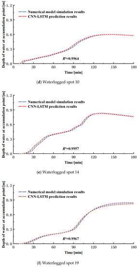
Figure 5.
Comparison of simulation results of the design rainfall scenarios based on the storm intensity formula.
When training machine learning algorithms, the selection of input parameters is very important. Reasonable optimization of the parameters can ensure the accuracy and precision of the model, and also enhance the timeliness of the model [23]. As can be seen from Figure 5, the coefficients of determination R2 are all above 0.95, indicating that the error between the ponding process predicted by the CNN−LSTM model and the hydrodynamic model was small. The design rain front r = 0.5, which peaked at the middle moment, shows that the ponding depth increased faster at 90 min, and then the ponding depth gradually tended to equilibrate with time. The waterlogging process pattern was basically similar at each waterlogging point. The results of the hydrodynamic model were derived from simulations such as rainfall data, while the results of the CNN−LSTM neural network model were derived from data-driven training of the hydrodynamic model. Both models provide a good response to the relationship between water depth and time at the water accumulation points. The predicted results were similar to the actual results.
The CNN−LSTM neural network model was selected to compare the predicted maximum ponding depths with the actual measurements based on the good design rainfall continuity in Chicago and the poor actual rainfall continuity. The model was used to predict the maximum ponding depth results for each ponding point during 20 July 2021 where no training was involved. The results of the comparison with the measured maximum ponding depths are shown in Table 3.
Table 3.
Comparison of measured and simulated water depths at inundated water accumulation points for 20 July 2021.
As seen in Table 3, the average error between the maximum ponding depth of the hydrodynamic model and the measured values was 5.20%. The average error between the predicted maximum ponding depth of the CNN−LSTM neural network and the measured values was 6.50%. The hydrodynamic model simulation results were used as training samples for the CNN−LSTM neural network, and thus by the accumulation of errors, but the difference was small. The actual rainfall continuity itself was poor, and the error between the CNN−LSTM neural network model and the hydrodynamic model was only 3.18%, satisfying a more accurate calculation accuracy.
In terms of time efficiency, the model took several hours to calculate 3 h of rainfall, as the speed of the hydrodynamic model was closely related to the number of grids and the size of the terrain. However, the neural network model did not need to consider these factors, and the CNN−LSTM neural network model took only 10 s. This is a significant time saving and can meet the needs of emergency flood control.
4. Conclusions
In this study, the CNN−LSTM neural network model and hydrodynamic model were used to construct a rapid prediction model for urban flooding in the central city of Zhoukou, and to achieve rapid prediction of urban flooding disasters. The main research findings are as follows.
(1) The main causes of waterlogging are excessive rainfall intensity, low-lying terrain, and insufficient drainage capacity of pipes. Therefore, the effects of rainfall, topography, pipe networks, and land use types are taken into account in the prediction model.
(2) The machine learning CNN−LSTM algorithm used in this paper has a good performance when making urban flooding predictions. The average error between the CNN−LSEM neural network prediction of the maximum ponding depth and the measured value is 6.50%, and the error between the CNN−LSTM neural network model and the hydrodynamic model is only 3.18%.
(3) After the hydraulic modelling and CNN−LSTM training, it only takes 10 s for the CNN−LSTM neural network model, which can buy a lot of lead time for emergency decision making and help decision makers to take better emergency management measures.
This paper proposes a CNN−LSTM-based fast prediction model for urban flooding depths, which can forecast the water depths of urban flood-prone spots more accurately and can provide an important scientific basis for urban disaster prevention and mitigation work.
Author Contributions
All of the authors contributed to the study conception and design. Writing and Editing: J.C. and Y.L.; Chart Editing: S.Z. All authors have read and agreed to the published version of the manuscript.
Funding
This research was funded by National Natural Science Foundation of China, grant number U22A20237.
Institutional Review Board Statement
Not applicable.
Informed Consent Statement
Not applicable.
Data Availability Statement
Data and materials are available from the corresponding author upon request.
Conflicts of Interest
The authors declare no conflict of interest.
References
- Shu, Z.; Li, W.; Zhang, J. Historicalchanges and future trends of extreme precipitation and high temperature in China. China Eng. Sci. 2022, 24, 116–125. [Google Scholar] [CrossRef]
- Kong, F. Countermeasures and insights from the 2012 Beijing “7.21” torrential rain and flooding disaster. China Disaster Reduct. 2022, 9, 42–45. [Google Scholar]
- Huang, J.; Li, M.; Kang, J. Social media-based rainstorm disaster information Real-time mining and analysis: Taking the 2019 “4.11 Shenzhen rainstorm” as an example. Water Econ. 2021, 39, 86–98. [Google Scholar]
- State Council Disaster Investigation Team. Investigation Report on the “7.20” Very Heavy Rainstorm Disaster in Zhengzhou, Henan Province; State Council Disaster Investigation Group: Beijing, China, 2022. [Google Scholar]
- Li, B.; Luo, H.; Chen, W. Risk assessment of storm water flooding in Minzhi area of Shenzhen based on numerical simulation. South-North Water Transf. Water Conserv. Sci. Technol. 2019, 17, 10. [Google Scholar]
- Harsha, S.; Agarwal, S.; Kiran, C. Regional flood forecasting using SWMM for urban catchment. Int. J. Adv. Technol. Eng. Explor. 2020, 9, 1027–1031. [Google Scholar] [CrossRef]
- Zhang, H.; Zhang, W.; Yang, W. Risk assessment of flooding in Ningbo sponge pilot area based on hydraulic drainage model. China Water Supply Drain. 2020, 36, 8–13. [Google Scholar]
- Sarkar, A.S.; Rahman, M.; Esraz-ul-zannat, M. Simulation-based modeling of urban waterlogging in Khulna city. J. Water Clim. Chang. 2020, 36, 8–13. [Google Scholar] [CrossRef]
- Li, P.; Xu, Z.; Zhao, G. Simulation of urban storm waterlogging based on SWMM and LISFLOOD-FP models: An example in Jinan City. South-North Water Transf. Water Conserv. Sci. Technol. 2021, 19, 1083–1092, (In Chinese and English). [Google Scholar]
- Ren, H.; Liu, S.; Xie, W. Characterization and risk assessment of urban flooding based on refined hydrodynamic model. Water Resour. Hydropower Technol. 2022, 53, 24–40. (In English) [Google Scholar]
- Kan, G.; Hong, Y.; Liang, K. Research on flood forecasting based on coupled machine learning models. China Rural. Water Conserv. Hydropower 2018, 10, 165–169+176. [Google Scholar]
- Liu, Y.; Liu, Y.; Zheng, J. Research on urban flood prediction method combining BP neural network and numerical model. J. Water Resour. 2022, 53, 284–295. [Google Scholar] [CrossRef]
- Mei, S.; Cheng, W.; Liu, G. A preliminary investigation of flood forecasting model based on support vector machine. China Rural. Water Conserv. Hydropower 2005, 3, 34–36. [Google Scholar]
- Hou, T.; Liang, H.; Huo, K. An Intelligent Internet of Things-based Urban A waterlogging monitoring and early warning system for Tianjin. Meteorol. Res. Appl. 2021, 42, 85–89. [Google Scholar]
- Li, H.; Wu, J.; Wang, Q. A machine learning approach for predicting rainstorm flooding in Shanghai. J. Nat. Hazards 2021, 30, 191–200. [Google Scholar]
- Pan, X.; Hou, J.; Chen, G. Rapid forecasting of urban flooding based on K-nearest neighbor and hydrodynamic model. Water Resour. Conserv. 2023, 1–17. [Google Scholar]
- Long, L.; Xu, H.; Ji, D. The Spatial and temporal characteristics of water temperature in Xiangjiaba Reservoir and its causes analysis. Yangtze River Basin Resour. Environ. 2017, 26, 738–745. [Google Scholar]
- Lecun, Y.; Bottou, L.; Bengio, Y. Gradient-based learning applied to document recognition. Proc. IEEE 1998, 86, 2278–2324. [Google Scholar] [CrossRef]
- Fu, G.S.; Liu, W.; Han, A. CNN-LSTM fusion network-based deep overflow early prediction learning method. China Pet. Mach 2021, 49, 16–22. [Google Scholar]
- Hochreiter, S.; Schmidhuber, J. Long short-term memory. Neural Comput. 1997, 9, 1735–1780. [Google Scholar] [CrossRef]
- Zhang, H.; Yang, S.; Guo, L. Comparisons of isomiR patterns and classification performance using the rank-based MANOVA and 10-fold cross-validation. Gene 2015, 569, 21–26. [Google Scholar] [CrossRef]
- Chen, J.; Li, Y.; Zhang, C. Urban Flooding Prediction Method Based on the Combination of LSTM Neural Network and Numerical Model. Int. J. Environ. Res. Public Health 2023, 20, 1043. [Google Scholar] [CrossRef] [PubMed]
- Hu, X.; Shi, L.; Lin, L. Improving surface roughness lengths estimation using machine learning algorithms. Agric. For. Meteorol. 2020, 287, 107956. [Google Scholar] [CrossRef]
Disclaimer/Publisher’s Note: The statements, opinions and data contained in all publications are solely those of the individual author(s) and contributor(s) and not of MDPI and/or the editor(s). MDPI and/or the editor(s) disclaim responsibility for any injury to people or property resulting from any ideas, methods, instructions or products referred to in the content. |
© 2023 by the authors. Licensee MDPI, Basel, Switzerland. This article is an open access article distributed under the terms and conditions of the Creative Commons Attribution (CC BY) license (https://creativecommons.org/licenses/by/4.0/).