Numerical Research on Migration Law of Typical Chlorinated Organic Matter in Shallow Groundwater of Yangtze Delta Region

Abstract

With the reform of China’s urbanization increasing in popularity, the security issues posed by urban groundwater, especially groundwater in industrial areas, have attracted scholars’ attention. This research aimed to predict and quantify the migration process of contaminants in a microconfined aquifer by conducting a groundwater contamination investigation in an abandoned chemical plant in the Jiangsu Province of China. First, data such as regional hydrogeological parameters and types of contaminants were obtained via hydrogeological drilling, groundwater well monitoring, pumping tests, and laboratory permeability tests, which helped identify the most serious pollution factor: chloroform. Then, a groundwater flow model was built using the Groundwater Modeling System (GMS) and verified using the general-purpose parameter estimation (PEST) package. In addition, based on the three-dimensional multi-species model for transport (MT3DMS) in GMS, a transport model was established. The results illustrate that the plume range of chloroform diffuses with water flow, but, because of its slow diffusion rate and inability to degrade naturally, the concentration of the contaminant has remained several times higher than the safety standard for a long time. The contaminant spread vertically to the soil layer above the microconfined aquifer under pressure, resulting in direct pollution. In addition, the contaminant in the microconfined aquifer is anticipated to migrate down to the clay layer and become enriched. However, the first confined aquifer has not been seriously polluted in the past 20 years. Finally, a sensitivity analysis of the parameters shows that groundwater contamination in the Yangtze delta region is greatly affected by precipitation recharge and hydraulic conductivity.

1. Introduction

Groundwater is an essential freshwater resource that is distributed globally [1,2] and is found in almost all human-intensive areas [3]. An increasing number of studies have indicated that groundwater is continuously polluted by human activities [4,5]. The contaminants in groundwater mainly include inorganic substances (heavy metals), organic substances, bacteria, and even radioactive sources, among which organic contaminants exert the most continuous and hazardous effects on environment [6,7]. The reason for this is that organic contaminants are slow to degrade naturally and are able to exist in the soil and groundwater for a long time. As one of the most developed regions in China, the soil and groundwater of many plots in the Yangtze delta region have been polluted by organic matter. The reason for this is that, with the development of the economy and the process of industrialization, a large number of chemical and pesticide production enterprises have been relocated, and there are organic pollution problems in the abandoned sites [8]. A study performed by Li shows that halogenated organics are the most severe contaminants in the groundwater and soil of China’s organic pollution sites [9]. Additionally, the halogenated organics are mainly chlorinated petroleum hydrocarbons (chloroform and 1,2-dichloroethane) [10]. Meanwhile, the compositions of aquifers in the Yangtze River Delta are regional. Taking Suzhou as an example, the groundwater mainly consists of shallow, middle, and deep aquifers (primarily in the first and second confined aquifers). The types of groundwater in shallow aquifer systems are phreatic and microconfined water [11]. Investigation studies have found that the organic pollution of groundwater in Suzhou is mainly concentrated in shallow aquifers, and microconfined aquifers have become the main source of domestic water in this area [8]. Therefore, for the health of residents, attention should be given to the safety of groundwater in shallow aquifers and, especially, to the investigation of the migration rules of contaminants in the groundwater of organically polluted sites. This should be done to provide guidance for the prevention and control of shallow groundwater contamination [12,13].

The key to preventing groundwater contamination lies in the timely prediction and identification of areas at risk of pollution. The Groundwater Modeling System (GMS) is a relatively mature software with a high accuracy in simulating groundwater flow and the transport of contaminants, which can aid in identifying at-risk areas, monitoring pollution, and blocking risk factors. Thus, it has been widely used [14,15].

Jesudhas applied a pollution transport model to predict the migration of total dissolved solids (TDS) in the Sengulam lake and then investigated possible risk factors in the Kodaganar river and the aquifers of the basin [16]. Based on the code of the three-dimensional multi-species model (MT3DMS) in GMS, Valivand developed a model to simulate the nitrate pollution of groundwater caused by agricultural activities and urban sewage [17]. Ahmed modeled the diffusion of contaminants in arid areas through generating a destination and migration model of heavy metals moving from the surface to groundwater [18]. Gedeon employed GMS to simulate groundwater flow by collecting data on the geology, hydrology, and rainfall of the study site, and then he constructed a contaminant transport model to predict the ammonium nitrogen and chloride levels of the Wang-Tien landfill site for ten years [19]. Ghoraba solved the problem of contaminant migration and time-varying concentrations in the central Nile Delta (El-Gharbiya Governorate), using a groundwater flow model (MODFLOW) and a data file from MT3DMS [20]. Based on the studies that have been mentioned, it can be seen that current research on the transport of contaminants mainly includes (i) predicting the transport behavior of contaminants from the surface source to the aquifer through soil, and (ii) predicting the concentration of contaminants at any point in the aquifer level through the migration of the aquifer at the horizontal plane [21]. Among types of aquifers, the unsaturated zone and phreatic aquifers have primarily been the focus of existing research. Microconfined aquifers have recently received growing attention, and researchers have become increasingly interested in studying these systems. For example, Song conducted a study on the changes in groundwater level fluctuations in the shallow confined aquifer of Hauraki coastal plain, New Zealand over the past 30 years. The study found that the groundwater level in this plain is influenced by various factors, including groundwater extraction, rainfall, and tides, with rainfall and groundwater extraction being the main drivers of groundwater level changes [22]. Li, on the other hand, investigated the groundwater fluctuations and ground settlement caused by dewatering in a coastal microconfined aquifer, using experimental data to establish corresponding mathematical models and exploring the effects of drainage rate and soil properties on the fluctuations and settlement [23]. However, it is worth noting that, while there have been many studies on microconfined aquifers, there have been relatively few studies on actual contaminated sites. Meanwhile, due to differences among regional and soil layer properties, there are few studies on shallow aquifers (especially microconfined aquifers) in East China, and the migration law of organic pollution in microconfined aquifers and its influence on adjacent aquifers are still unclear. In addition, previous studies have mostly assumed that areas around the sites of pollution leakage are harmed after the leakage, and have lacked comprehensive investigations into and research on the actual polluted sites. Therefore, using an actual organic pollution site in the Yangtze Delta region of East China, this study simulated the migration behavior of typical chlorinated petroleum hydrocarbons (chloroform) in a microconfined aquifer and its influence on other adjacent aquifers. With the cases investigated, this study intends to gain a deeper insight into the treatment of organic pollution sites in the Yangtze Delta region.

This research was performed as follows. (i) A groundwater flow model was established according to the hydrogeological characteristics of the site, which was obtained from hydrogeological drilling, geophysical prospecting, field pumping tests, and laboratory analysis. (ii) The groundwater flow model was verified and calibrated through the general-purpose parameter estimation (PEST) package in GMS. (iii) The MT3DMS code was employed to model the transport of groundwater contamination, predict the spatial distributions of the contaminant in the next 20 years, and observe the migration of contaminants between different aquifers. (iv) The environmental factors exerting the greatest impact on the migration of contaminants were explored through a parameter sensitivity analysis.

2. Information on the Study Site

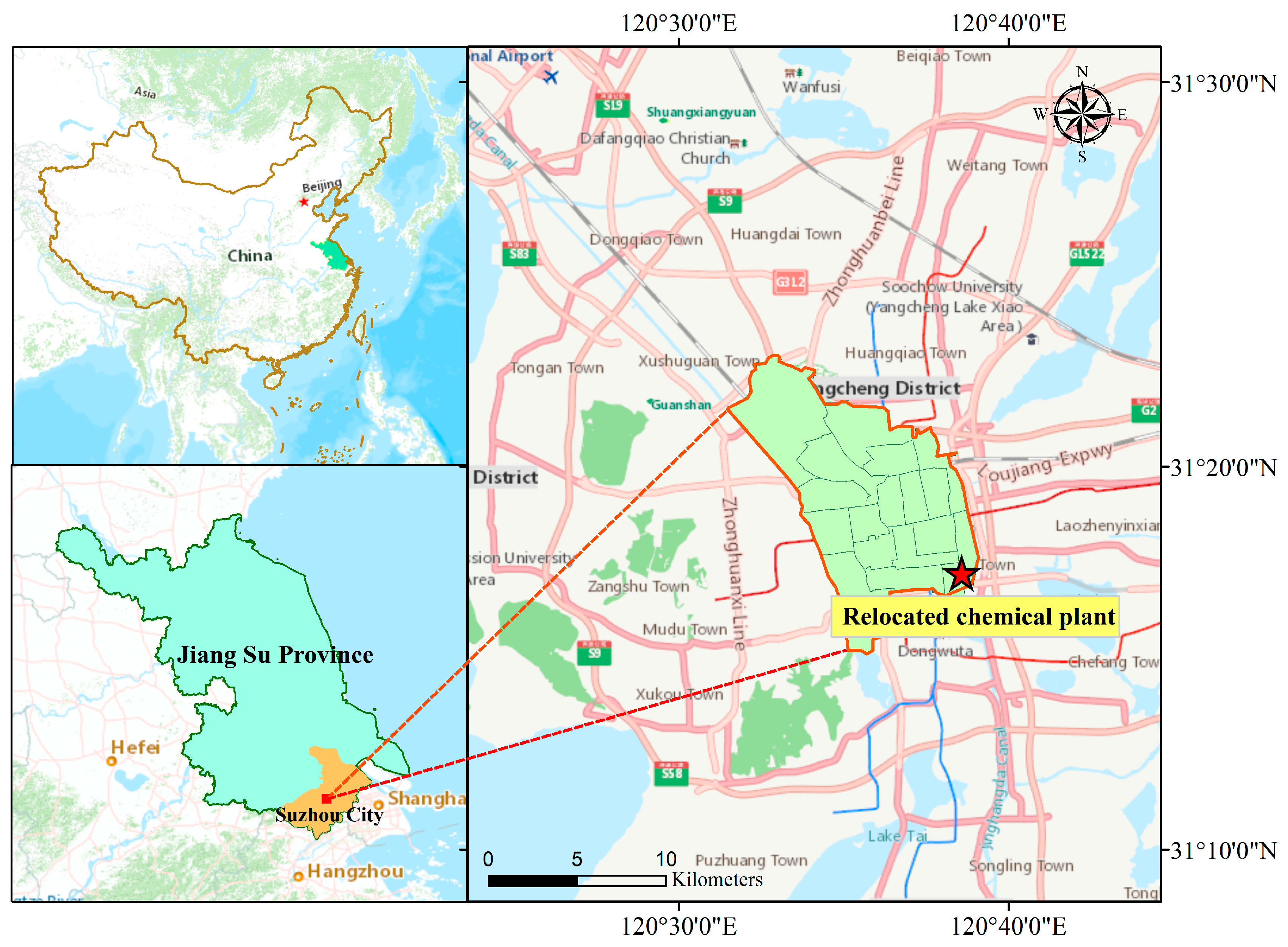
2.1. Description of the Study Site

The study site, located in the city of Suzhou, southeast of the Jiangsu Province of China (Figure 1), extends between the longitudes 120°38′13″ E and 120°38′31″ E and latitudes 31°16′59″ N and 31°17′6″ N, and occupies a total area of 108,123 m². As a part of the water network plain of Taihu Lake, it is adjacent to the Qingyang River in the north and Old Canal in the east. The site’s elevation ranges between 2.0 m and 5.0 m, meaning it is flat with no apparent topographic fluctuations. Suzhou is in a typical subtropical monsoon climate zone, which is humid and rainy, with monsoons and four distinct seasons. Between 2010 and 2020, the average annual precipitation in Suzhou was 1030.6 mm/year, and the average annual evaporation was 1420.3 mm/year.

2.2. Data Measurement and Collection from the Site

Following the method described in the Technical Guideline for Site Soil and Groundwater Sampling of Volatile Organic Compounds (HJ1019-2019) from April 2021 [24,25], an initial investigation was conducted at the site. To obtain the properties of the subsurface soil layers and observe regular changes in the groundwater head, different types of boreholes were drilled at the site. There are 9 hydrogeological boreholes and 18 groundwater head monitoring wells with depths of 24.0 m and 21.0–22.5 m, respectively. In addition, two groups of pumping-test wells were arranged on site to obtain the hydrogeological parameters. Each pumping-test group was composed of one pumping well and two observation wells. At the same time, a total of 83 groundwater pollution-monitoring wells (including 15 shallow wells with a depth of 8.0 m, 58 deep wells with a depth of 18.0 m, 5 deep wells with a depth of 20.0 m, and 5 deep wells with a depth of 22.5 m) were set up to monitor the concentration of groundwater contaminants.

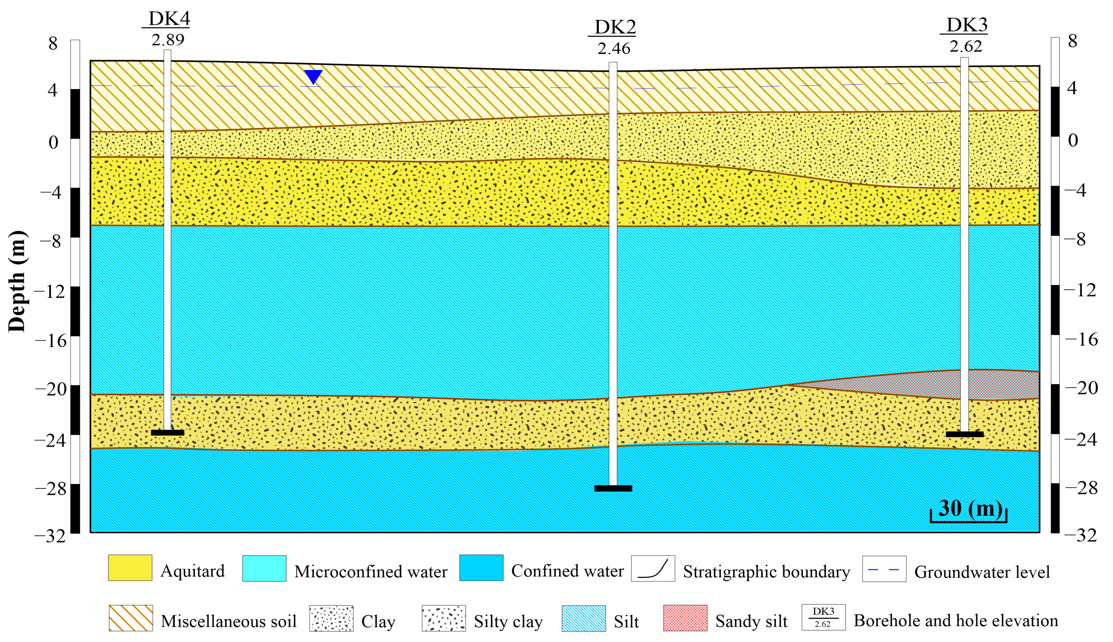
2.3. Hydrogeological Conditions of the Site

According to the geological survey report and the nature of the soil layer, the alluvium below the surface of the study area can be divided into five categories: miscellaneous soil, clay, silty clay, silt, and sandy silt, as shown in Figure 2. In addition, the groundwater is mainly found in silt and sandy silt. The former is called microconfined water and the latter is first confined water. The microconfined aquifer is located at 9.0–18.0 m below the surface. It was found that the roof lithology of the microconfined aquifer is mainly clay and silty clay, its pore ratio is 0.745–0.804, its water content is 26.5–28.7%, its compression coefficient is 0.16–0.59 Mpa, and its compression modulus is 3.72–10.31 Mpa. The soil at the study area all has a medium–high compressibility and a certain pressure bearing, which is in line with the investigation and research results of Shi [26]. The first confined aquifer is located 4.0–8.0 m below the microconfined aquifer, and a weak, permeable layer composed of clay separates it from the microconfined aquifer. However, there is a hydraulic connection between the two aquifers, so both aquifers are worthy of attention when pollution occurs.

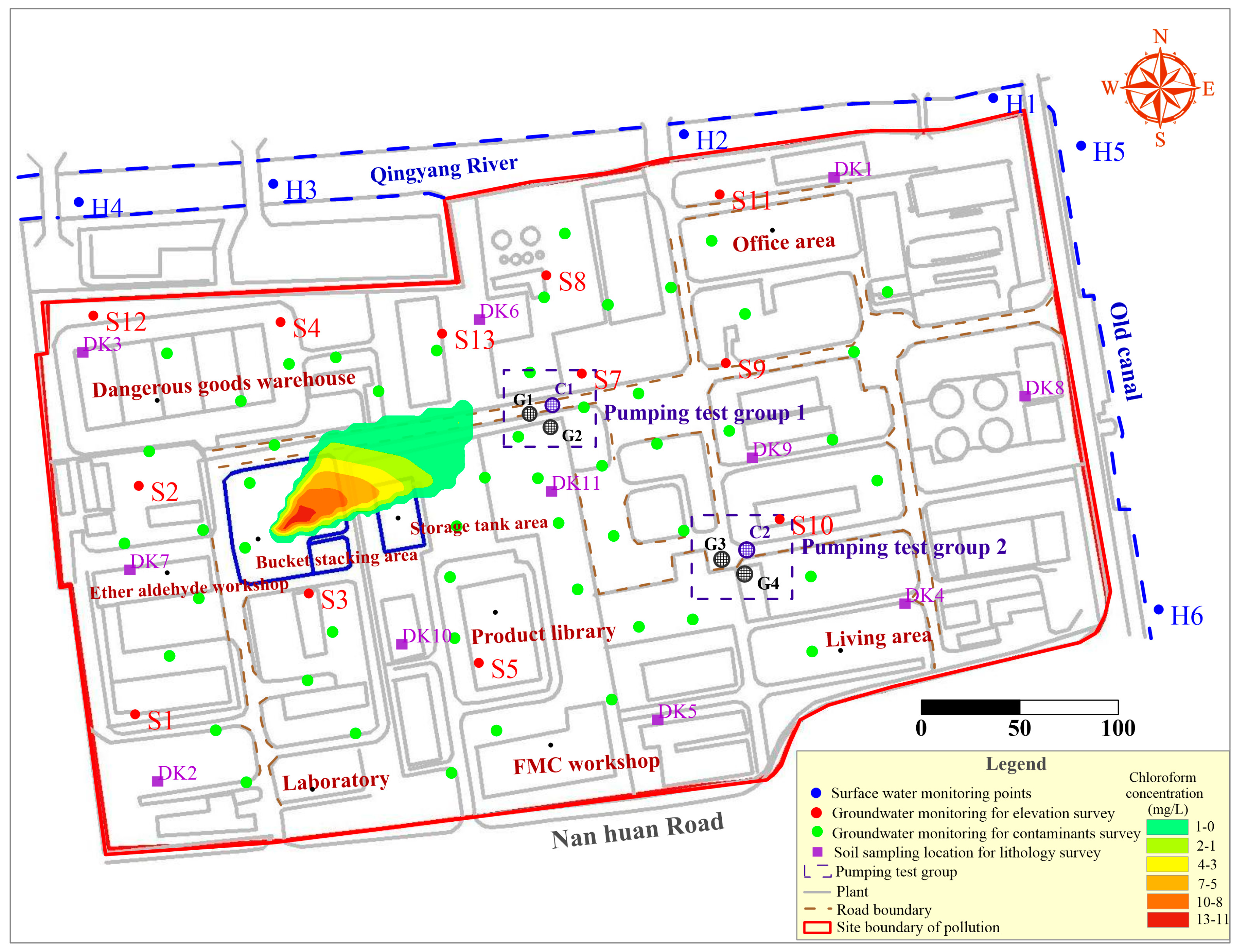
2.4. Survey of Groundwater Contamination

Before relocating, a solvent factory that produced plasticizers, diphenyl ether, hydrogenated terphenyl, and other chemicals was located at the research site. The main raw materials used during production were chlorinated benzene, carbon tetrachloride, phosphorus trichloride, chloroform, and other organic compounds. The plant had been working for 30 years before its move. During the investigation, contaminants were sampled and tested through groundwater-monitoring wells. From 4 August to 25 December 2021, 5 batches of groundwater samples were collected, and 200 samples were submitted for inspection in each batch. Multiple sample tests show that the plot is mainly polluted by organic matters, among which the most important organic contaminants are benzene, carbon tetrachloride, chloroform, and chlorobenzene. These results are listed in

Table 1. Contaminant concentrations in groundwater-monitoring wells.

Contaminants	Risk Control Value (mg/L)	Maximum Pollution Concentration (mg/L)	Maximum Exceedance Multiple	Main Distribution Depth (m)
Benzene	0.84	87.36	103.00	5.00–15.00
Carbon Tetrachloride	0.13	16.13	125.00	5.00–15.00
Chlorobenzene	5.79	509.08	87.00	9.00–15.00
Chloroform	0.05	17.92	223.00	9.00–18.00

, including the maximum pollution concentration, maximum exceedance multiple, and main distribution depth. It can be seen that benzene, chlorobenzene, chloroform, and carbon tetrachloride levels in the groundwater substantially exceed the standard; these are mainly concentrated in the microconfined aquifer. There are three potential reasons for this: (i) The sediment at the bottom of the sewage-regulating tank of the original factory was randomly stacked in the site during the demolition of the building, and no effective anti-seepage measures were taken. (ii) The careless excavation of civil works occurred during factory construction over the years, resulting in leakage from process pipelines and of production materials along the foundational pit of the infrastructure. (iii) There was no major environmental accident at the plant, but excessive production was performed by the old chemical enterprise. These potential reasons are known to cause serious pollution in groundwater, especially the first; through rainfall infiltration, contaminants from the surface down to the microconfined aquifer sewage are enriched. Previous investigations have found that halogenated organic compounds (84%), benzene series (49%), and petroleum hydrocarbons (20%) are the top three main contaminants in the groundwater of organic pollution sites in the Suzhou area. The halogenated organic compounds are chlorinated petroleum hydrocarbons (chloroform: 20%; 1, 2-dichloroethane: 31%) and chlorobenzene organic compounds [27]. Because the main pollutant in the microconfined aquifer of the study area is chloroform, and because its density is 1.48 g/cm³, which is higher than that of water and allows it to more easily migrate downward in aquifers to pollute the next aquifer, chloroform was selected as the main contaminant in this study to predict its migration in groundwater.

3. Methodology

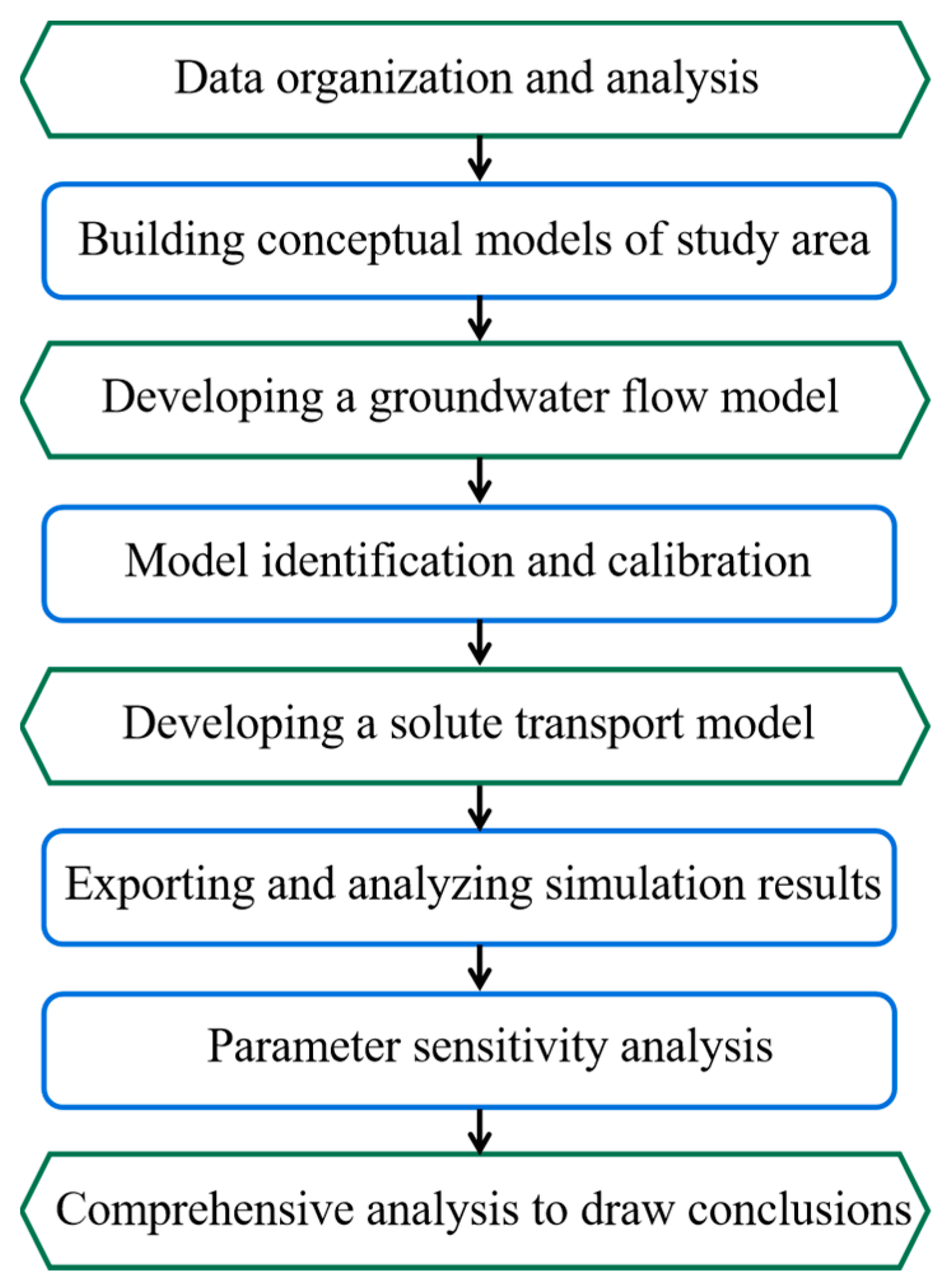
3.1. Research Process

The main research process of this study consisted of several stages: (i) the collection and analysis of hydrogeological data from the study area; (ii) the development of a groundwater flow model; (iii) the establishment of a solute transport model; and (iv) a comprehensive analysis of the simulation results. The detailed research process can be seen in the following Figure 3.

3.2. Groundwater Flow Equation

The partial differential equation solved numerically in MODFLOW is as follows [28]:

$$\{\begin{array}{l}\frac{\partial }{\partial x}\left(k_x\frac{\partial H}{\partial x}\right)+\frac{\partial }{\partial y}\left(k_y\frac{\partial H}{\partial y}\right)+\frac{\partial }{\partial z}\left(k_z\frac{\partial H}{\partial z}\right)+G=u_s\frac{\partial H}{\partial t}(x,y,z)\in \mathrm{\Omega }\\ H(x,y,z,t)=H_0(x,y,z),(x,y,z)\in \mathrm{\Omega },t=0\\ H(x,y,z,t){|}_{B_1}=H_1(x,y,z,t),(x,y,z)\in B_1,t>0\\ K\frac{\partial H}{\partial \overrightarrow{n}}{|}_{B_2}=q(x,y,z,t)=0,(x,y,z)\in B_2,t>0\end{array}$$

(1)

where k_x, k_y, and k_z are the hydraulic conductivity values along the x, y, and z coordinate axes (LT⁻¹); G is the volumetric flux per unit volume representing the sources and sinks of groundwater (T⁻¹); H is the hydraulic head in the flow domain of the simulation (L); u_s is the specific storage capacity of the investigated aquifer; t is time (T); B₁ is the boundary interface of the constant head (first type boundary); B₂ is the flow boundary (second type boundary); H₀(x,y,z) refers to the hydraulic head of the boundary and the internal flow domain at the initial moment; H₁(x,y,z) represents the hydraulic head in the flow domain of the first type boundary; q is the unit discharge from the flow domain of the second type boundary (L³T⁻¹L⁻²); $\overrightarrow{n}$ is the direction of the outer normal of the boundary; and K_n is the hydraulic conductivity in the normal direction of the boundary (LT⁻¹).

3.3. Contaminant Transport Equation

Since solute transport adapts to Fick’s Law, the partial differential equation of groundwater contamination can be integrated with models of groundwater flow and solute transport through the motion Equation (2) [29]:

$$\{\begin{array}{l}R\theta \frac{\partial C}{\partial t}=\frac{\partial }{\partial x_i}(\theta D_{ij}\frac{\partial C}{\partial x_j})-\frac{\partial }{\partial x_i}(\theta V_{i}C)-W{C}_s-WC-{\lambda }_1\theta C-{\lambda }_2{\rho }_b\overline{C}\\ R=1+\frac{{\rho }_b}{\theta }\frac{\partial \overline{C}}{\partial C}\\ C(x,y,z,t)=C_0(x,y,z),(x,y,z)\in \mathrm{\Omega },t=0\\ C(x,y,z,t){|}_{s_1}=c(x,y,z,t),(x,y,z),(x,y,z)\in S_1,t>0\end{array}$$

(2)

where R is the hysteresis coefficient, dimensionless; θ represents the porosity of the porous medium, dimensionless; ρ_b is the density of the porous medium (ML⁻³); C_s is the dissolved concentration of contaminants (ML⁻¹); C is the pollutant concentration (ML⁻¹); $\overline{C}$ is the solid phase adsorption concentration of contaminants (ML⁻¹); D_ij is the hydrodynamic dispersion coefficient tensor (L²T⁻¹); V_i is the seepage or linear pore water velocity based on the Darcy equation (LT⁻¹); λ₁ is the first-order reaction rate of the dissolved phase (T⁻¹); λ₂ is the reaction rate of the adsorbed phase (LM⁻¹T⁻¹); C₀(x,y,z) is the concentration distribution of known contaminants; S₁ is the boundary for a given concentration; c(x,y,z) is the concentration distribution on this boundary. Based on the hydrogeological conditions of the study area, the simulation only assessed the effects of solute transport on advection and diffusion, thus adsorption and other factors were not considered [30].

3.4. Parameter Sensitivity Analysis Method

Parameter sensitivity analyses can be used to analyze the migration processes of pollutants and evaluate the sensitivity of different parameters of transport behavior. This approach allows for a deeper understanding of how environmental factors impact pollutant migration and of the behavioral characteristics of pollutants under varying environmental conditions. Commonly used sensitivity analysis methods include the local analysis method, the global analysis method, the mathematical method and the graphical method [31], among which the local analysis method is the most widely accepted. The local analysis method only tests the influence of a single parameter on the model. Therefore, this study used the local analysis method for the sensitivity analysis. The calculation formula is as follows

$$SAF=\frac{\Delta A/A}{\Delta F/F}$$

(3)

In the formula, ΔA/A is the rate of change for the uncertainty factor and ΔF/F refers to the rate of change for the evaluation index; an SAF of >0 means that the evaluation index and the uncertainty factor change in the same direction, and an SAF of <0 means that the evaluation index and uncertainty factor change in the opposite direction. The larger the SAF, the more sensitive the evaluation index F is to the uncertainty factor A, and vice versa.

4. Construction of the Numerical Model

4.1. Numerical Simulation of Groundwater Flow

The conceptual model of groundwater generalizes the complicated geology into several aquifers and aquitards and keeps the mainstream particularities of groundwater movement. It mainly includes a hydrogeological structure generalization, a boundary generalization, a parameter generalization, and a flow-field generalization.

4.1.1. Hydrogeological Structure Generalization

This research intends to model an accurate groundwater flow field for the site and then simulate the migration of contaminants in the groundwater in both horizontal and vertical directions. Therefore, according to the soil conditions of the site, the hydrogeological structure is generalized. That is, the stratum is divided into aquifers and aquitards, which are, from top to bottom, the phreatic aquifer, the first aquitard layer, the microconfined aquifer, the second aquitard layer, and the first confined aquifer.

4.1.2. Model Discretization

In order to solve the mathematical model of aquifers using the finite difference method, it is necessary to divide the layers of the model into standard cells with an appropriate size and shape. To avoid interpolation errors from the boundary grids in calculating the initial conditions of the model, the site was extended to a 500.0 × 400.0 m rectangular structure covering, approximately, the entire study area. This was discretized into 100 rows and 100 columns with a grid size of 5.0 × 4.0 m, resulting in a total of 50,000 grid cells, of which 31,375 cells were active. In the vertical direction, according to the drilling data, the elevation between the model bottom and the ground surface was about 40.0 m thick, which can be broken down into five different thicknesses, namely five different soil layers. The simulation of the preset model lasted from April 2021 (the groundwater level and pollution investigation on the site began at that time) to March 2022, and the calculation time step is one day.

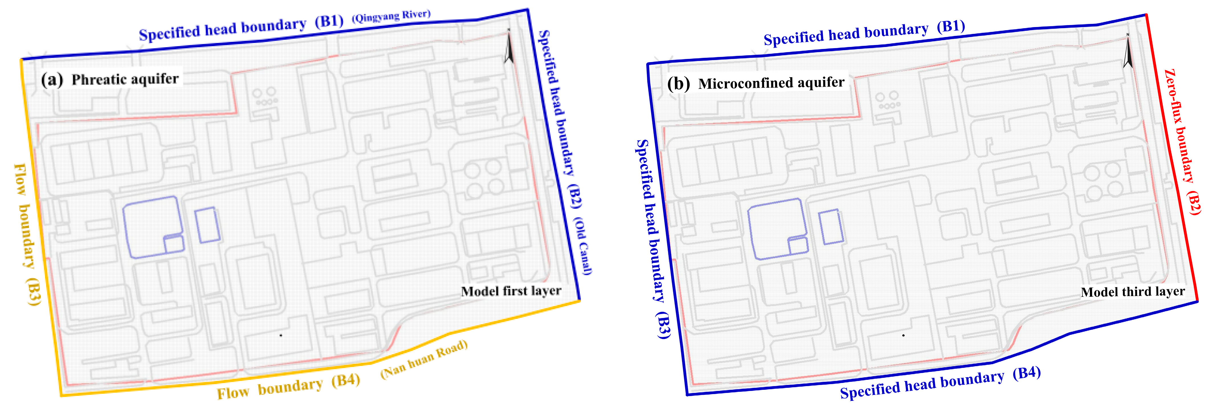
4.1.3. Boundary Condition

The northern and eastern borders of the site are adjacent to the Qingyang River and Old Canal, respectively, both of which have water heads that are relatively stable throughout the year. Meanwhile, the field investigation found that the depth of the two rivers is from 3.0 to 5.0 m, which is close to that of the diving layer but has no obvious connection with the microconfined aquifer. Based on water head survey data from the two rivers for a one-year period, the boundaries of the model phreatic aquifer were identified as the constant head boundaries using the time-varying specified head package (CHD) of the MODFLOW code. There were no obvious natural boundaries between the western and southern halves of the study site, thus, these boundaries are generalized as artificial flow boundaries. The flow rate of each boundary in each aquifer was calculated using the aquafer’s hydraulic conductivity and hydraulic gradient measured on site. The initial water level of the microconfined aquifer was preset based on the site’s groundwater survey data (Figure 4). Vertically, the ground surface, as the upper boundary of the model, receives rainfall infiltration, recharge, and evaporation. The lower boundary is the bottom plate of the first confined aquifer.

However, it should be noted that when setting the boundary conditions, the relatively simple geological and hydrological conditions of the study area, which is located in a plains area, make setting the boundary conditions relatively simple. In addition, there are no other factors, such as groundwater extraction and river cutting, that can cause water flow exchange, and thus the groundwater conditions in the microconfined aquifer are relatively stable and simple. Therefore, this model can reflect relatively common and simple confined aquifer conditions in the Yangtze River Delta plains area. However, for microconfined aquifers with complex terrain structures or other artificial groundwater treatment conditions, the model used in this study has certain limitations. For more complex site conditions, further model adjustments may be needed to improve accuracy.

4.1.4. Initial Conditions and Parameter Setting

In order to obtain more accurate rates of hydraulic conductivity in the microconfined aquifer, two sets of pumping tests were set up at the site around the fully cased wells. The depth of both the pumping and observation wells was 24.0 m; filter holes were drilled at 16.0–20.0 m deep in the wells, and the lower part is a sedimentation pipe filled with clay balls to stop water above 16.0 m. Each group of tests was conducted three times in turn, and the results are shown in

Table 2. Results of the pumping tests at the aquifers.

Position	Order	r1 (m)	r2 (m)	M (m)	Q (m3/d)	S1 (m)	S2 (m)	R (m)	Permeability (m/d)	Average Value (m/d)
Group 1	1st time	8.00	14.00	1.60	15.10	1.55	0.54	17.00	0.83	0.75
	2nd time	8.00	14.00	1.60	9.49	0.96	2.13	16.00	0.68
	3rd time	8.00	14.00	1.60	5.17	0.52	1.94	17.00	0.73
Group 2	1st time	6.00	12.00	2.00	8.44	1.57	0.65	14.00	1.06	0.85
	2nd time	6.00	12.00	2.00	5.65	1.02	1.62	14.00	0.74
	3rd time	6.00	12.00	2.00	2.87	0.52	1.43	14.00	0.75

. In coordination with the results of the pumping tests, the equation used in the test method (Equation 4) was independently employed to estimate hydraulic conductivities. The pumping test results show that the hydraulic conductivities of the microconfined aquifers in the study area were between 0.68 m/d and 1.06 m/d. Furthermore, after extracting soil samples from different layers through soil drilling at the site, laboratory tests were carried out to acquire the various hydrogeological parameters of the different soil layers. Through combining the results of the laboratory tests with regional engineering experience, these parameters (such as the rainfall infiltration coefficient, porosity, and longitudinal dispersion coefficient) were identified. They are given in

Table 3. Hydrogeological parameters in the model.

Layer Number	Horizontal Conductivity (m/d)	Vertical Conductivity (m/d)	Effective Porosity	Longitudinal Dispersity (m)
1	0.0173	0.0259	0.483	10.0
2	0.0023	0.0031	0.427	8.0
3	0.7500	0.7000	0.464	15.0
4	0.0369	0.0420	0.469	10.0
5	0.7900	0.7530	0.486	20.0

and assigned to the model:

$$\{\begin{array}{l}K=\frac{0.366Q\lg (r_2/r_1)}{M(S_1-S_2)}\\ \lg R=\frac{D_1\lg r_2-D_2\lg r_1}{D_1-D_2}\end{array}$$

(4)

where K is specified as the permeability of the aquifer (LT⁻¹); Q is the pumping flow (L³T⁻¹); D₁ and D₂ are the draw-downs of the two observation logs (L); r₁ and r₂ are the distances from the two observation wells to the pumping well (L); R is the pumping influence radius (L); and M is the thickness of the aquifer (L).

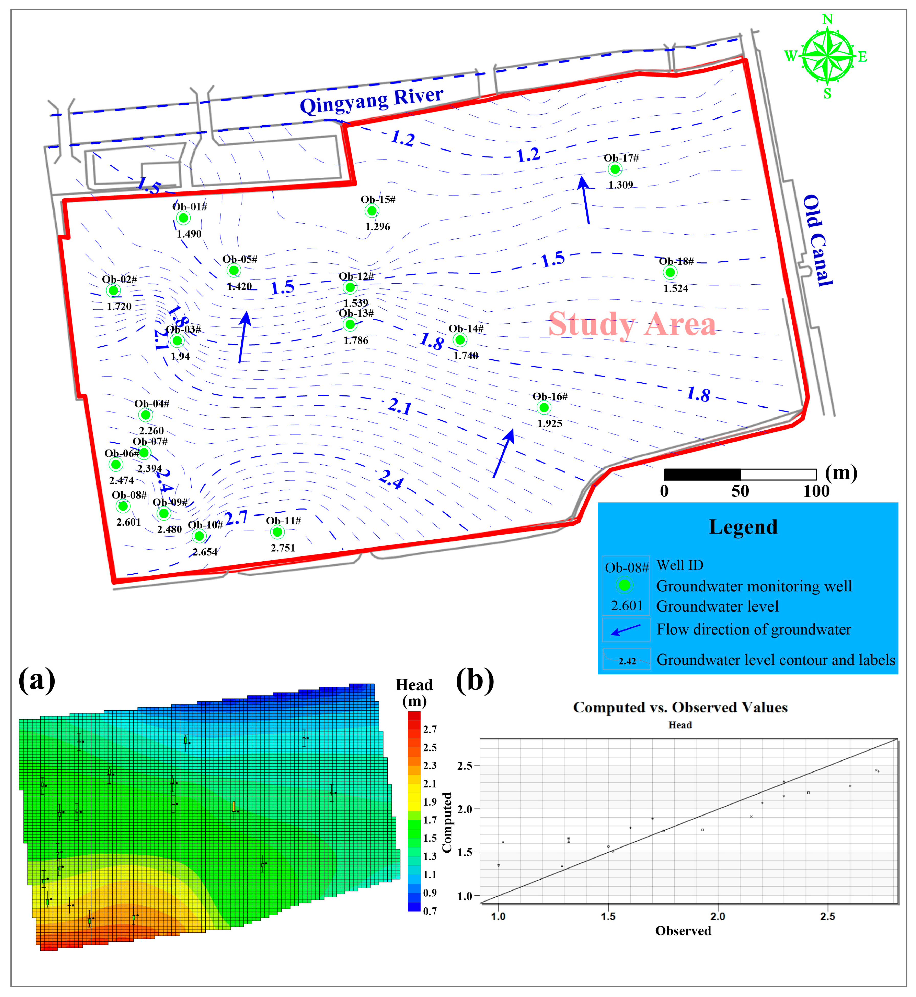
4.2. Flow Model Verification and Calibration

Model calibrations were needed to adjust the parameters until the mean difference between the values of the simulated and field observations met accuracy requirements. This ensures that the model has the ability to reproduce the real behavior of the system. While the microconfined aquifer is the main focus of this study, the investigation found that its phreatic water level was affected by on-site construction and other factors, meaning it can be relatively erratic and cannot be used as a reference for the calibration of the flow field. Therefore, the water-level measurement in the microconfined aquifer was selected as the calibration standard, and the hydraulic conductivity of the microconfined aquifer in the model was corrected using the general-purpose parameter estimation (PEST) package in the GMS software [32]. The survey data show that the head of the microconfined aquifer is stable all year round, with the fluctuation in the water level generally within 0.5 m. Consequently, this research used the microconfined groundwater heads, taken in June 2021, as the calibration heads for parameter identification. Then, the PEST inverse calculus program was used to compare water heads between the simulation and observation, thus obtaining more precise modeling results. Figure 5 shows the head contour of microconfined water in June 2021, which suggests that the groundwater flows from southwest to northeast with a small hydraulic gradient. Figure 5a exhibits the calculated groundwater flow field after parameter calibration. The difference between the observation water heads and the calculated water heads is within the confidence interval. Additionally, the flow direction is consistent with the measured flow field. Simultaneously, Figure 5b demonstrates the similarities between the computed and observed values, and the values on the 45-degree line describe correspondence. The above results illustrate that the calibrated model can better reflect the actual flow-field characteristics of the study area.

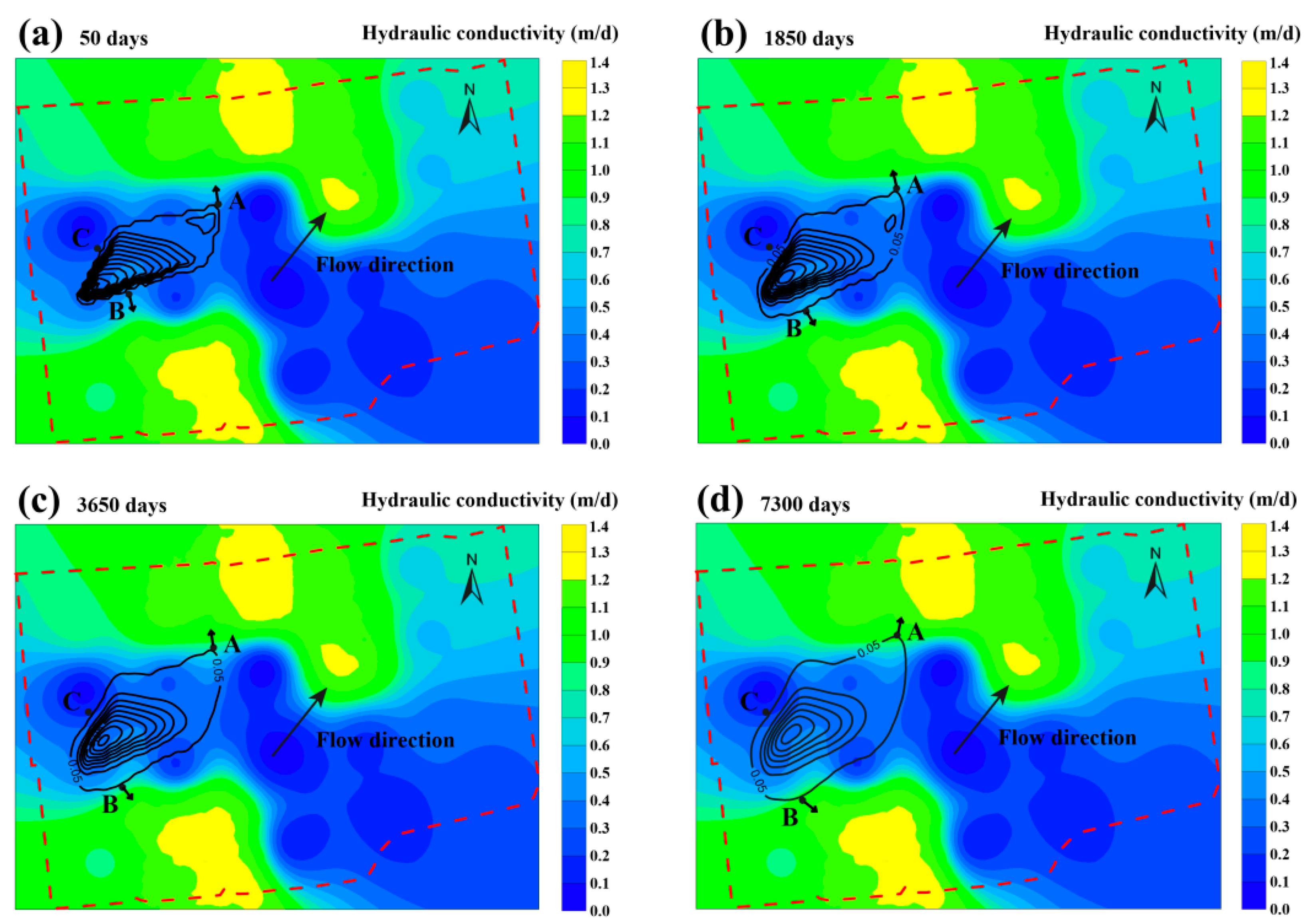
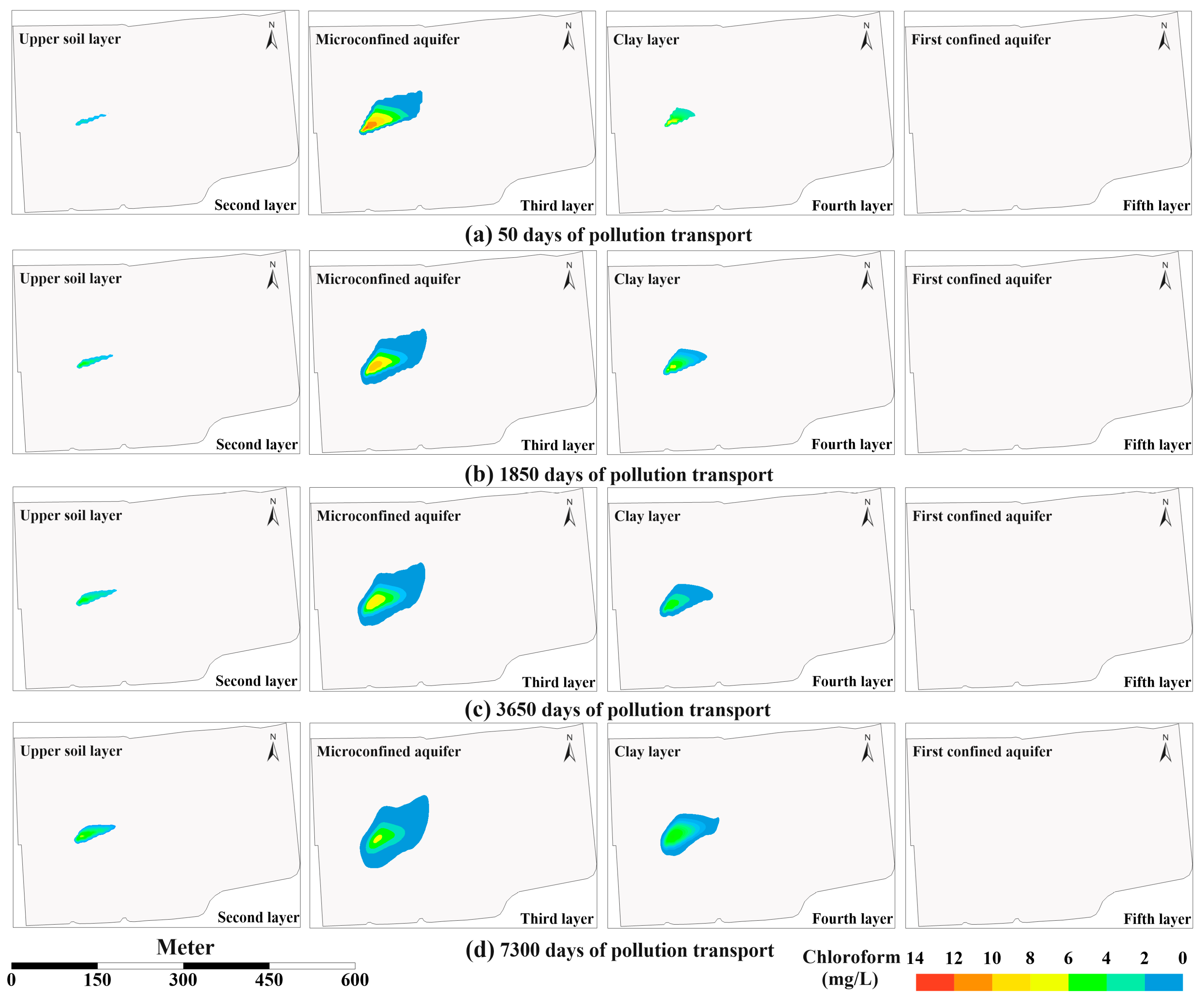
4.3. Numerical Simulation of Groundwater Contaminant Transport

The solute transport model was based on a calibrated water flow model. By coupling the MT3DMS with the flow simulation results of MODFLOW, this study sets the characteristic parameters of the transport model (porosity, hydrodynamic dispersion coefficient, etc.), the initial concentration of contaminant, and the simulation period. Based on the concentration of chloroform, the Kriging interpolation method was used to calculate the concentration contour in the study area, as shown in Figure 6. This shows that chloroform pollution was primarily distributed in the factory’s original barrel stacking and storage tank area. The most significant pollution point was in the barrel stacking area, which may have been caused by a lack of protective measures for sample leakage during the storage and use of chemicals. The next step was to input the initial concentration of chloroform into the model. To avoid the risk of skewed data during the transportation process, only the influence of groundwater convection and diffusion was considered, and the adsorption and biodegradation reactions were not. The simulation period was preset as 20 years and the time step was 50 days.

5. Results and Discussion

Based on the distribution of pollutant concentrations obtained using interpolation, after adjustment and calibration, the solute transport model was used to predict the plume diffusion of pollution and trends in the changes to concentrations of chloroform in the microconfined aquifer over the next 20 years (2021–2041). Figure 7 indicates changes to the shape of the pollution plume of groundwater chloroform after 50, 1850, 3650 and 7300 days. According to the quality standard for groundwater (GB/T14848-93), 0.05 mg/L is taken as the pollution risk control value to show the migration trend and impact range of contaminants. It can be seen from the Figure 7 that the pollution range increased significantly in the simulated 20 years, from the initial 4664.92 m² (50 days) to 7504.30 m² (7300 days), with an average annual increase of 142.95 m². Moreover, the area of the pollution plume in the northeast increased rapidly, and the isolines of pollution concentration became more dispersed. The reason for this is that the water flow from the microconfined aquifer flows from southwest to northeast, and the chloroform dissolved in groundwater migrates along the water flow. However, it is worth noting that the pollution plume develops in an irregular shape, resulting from the non-homogeneous hydraulic conductivity field of the microconfined aquifer generated using the PEST reverse calculus template in the process of verification and identification. Under the influence of the non-homogeneous field, the transport of contaminants is not uniform [33]. It can be seen from the Figure 7 that the hydraulic conductivity distribution of the simulated field is 0.3–1.2 m/d, and the hydraulic conductivity of the upper part of the simulated field and the lower left part are significantly larger than the value of the middle part of the simulated field. Although the hydraulic conductivity of the field cannot be completely restored, the inversion value is consistent with the value obtained from the field pumping test, and the error is within a certain range, which can be used as a reference for the actual hydraulic conductivity field. By observing the trends in the variation of pollution isolines at three points (A, B, and C) in the pollution plume, we can find that the contaminants migrate to areas with relatively high hydraulic conductivities, point A and point B, on the premise of maintaining diffusion along the water flow. However, the density of the isolines at point C does not change much, and diffusion is inhibited by low hydraulic conductivity. It can be seen that contaminants easily migrate to soil layers with high hydraulic conductivities, which is consistent with the research results produced by Chen [25]. However, since the microconfined aquifer is mainly composed of silty clay and some silty sand, and since its overall hydraulic conductivity coefficient is low and its hydraulic gradient is less than 1‰, the pollutant transport has not exceeded the plant area in 20 years; thus, the pollution risk in the horizontal direction is low.

The microconfined aquifer in the study area is adjacent to the phreatic aquifer and the first confined aquifer. Therefore, what deserves the attention of site restorers is whether the contaminants in the microconfined aquifer will migrate to other aquifers and cause serious pollution. The predicted pollution levels of the two soil layers adjacent to the microconfined aquifer and the first confined aquifer in the next 20 years are shown in Figure 8. The soil layer above the microconfined aquifer has been excavated and cleaned by contaminated soil and backfilled in the early stage, so this part of the soil can be regarded as clean soil. The pollutant concentration in the microconfined aquifer can be used as the initial concentration boundary of the adjacent soil layer. According to the simulation results, the maximum concentration of contaminants in the microconfined aquifer shows a downward trend, but the rate of decline is 0.228 mg/L/year (see

Table 4. Numerical simulation results for the transport model of the microconfined aquifer.

Migration TIME (day)	Contaminated Area (m2)	Variable Quantity (m2)	Maximum Concentration (mg/L)	Variable Quantity (mg/L)	Upward Migration Distance (m)	Variable Quantity (m)	Vertical Migration Depth (m)	Variable Quantity (m)
50	4664.92		13.27		0.40		1.50
1850	5767.56	1102.64	10.87	−2.40	0.90	0.50	2.00	0.50
3650	6449.74	682.18	9.99	−0.88	1.40	0.50	3.00	1.00
5450	7019.51	569.77	9.34	−0.65	1.70	0.30	3.70	0.70
7300	7504.30	484.79	8.71	−0.63	1.90	0.20	4.80	1.10

for specific pollution data). It can be seen that, under natural conditions, the degradation rate of contaminants in the aquifer with a low hydraulic conductivity is slow, and it is impossible to rely on migration to alleviate the pollution degree. Meanwhile, in addition to horizontal transport, attention should also be paid to vertical transport of contaminants. According to Figure 8, contaminants in the microconfined aquifer will have an impact on the two adjacent soil layers. The main reason for the pollution of soil above the confined aquifer is that the upper roof of the microconfined aquifer has a certain pressure, and the contaminants will migrate upward under the joint action of capillary force and stress, sending pollution to the clean top soil. However, the density of chloroform is greater than the water and its impact on the upper layer soil is limited, so the pollution range is relatively constant in the later stages of the simulation. Below the microconfined aquifer, there is a first confined aquifer separated by a silty clay layer. As a result of the Earth’s gravitational pull, contaminants will migrate downward, and the silty clay layer (aquitard) will be mainly polluted by chloroform while the first confined aquifer will not be polluted. The reason for this may be that the hydraulic conductivity of the clay layer is only 0.03 m/d, making it a weakly permeable layer, which restricts the downward migration of chloroform to the first confined aquifer [34]. Additionally, the chloroform that migrates downward will be enriched in silty clay layers; therefore, silty clay layers can be regarded as a natural barrier to protect the first confined aquifer from contamination. However, it is still necessary to be vigilant against contaminants that may penetrate the aquitard and reach the first confined aquifer at a long-enough time scale.

To sum up, in the low hydraulic conductivity zone of the Yangtze River Delta, the migration rate of contaminants in the microconfined aquifer is very slow with a limited range of the horizontal diffusion of contaminants, which does not pose a serious risk. However, the contaminants are difficult to degrade naturally and have high densities. Apart from water flow, hydraulic conductivity also determines the migration direction of contaminants. In areas with high hydraulic conductivities, contaminants migrate easily. Therefore, in the course of treatment for contaminated aquifers, we should draw attention not only to the direction of water flow but to the soil layer with a high hydraulic conductivity where reverse flow diffusion may exist [35]. Last but not least, since the confined aquifer has confined characteristics, the upward transport of contaminants is also worthy of studying.

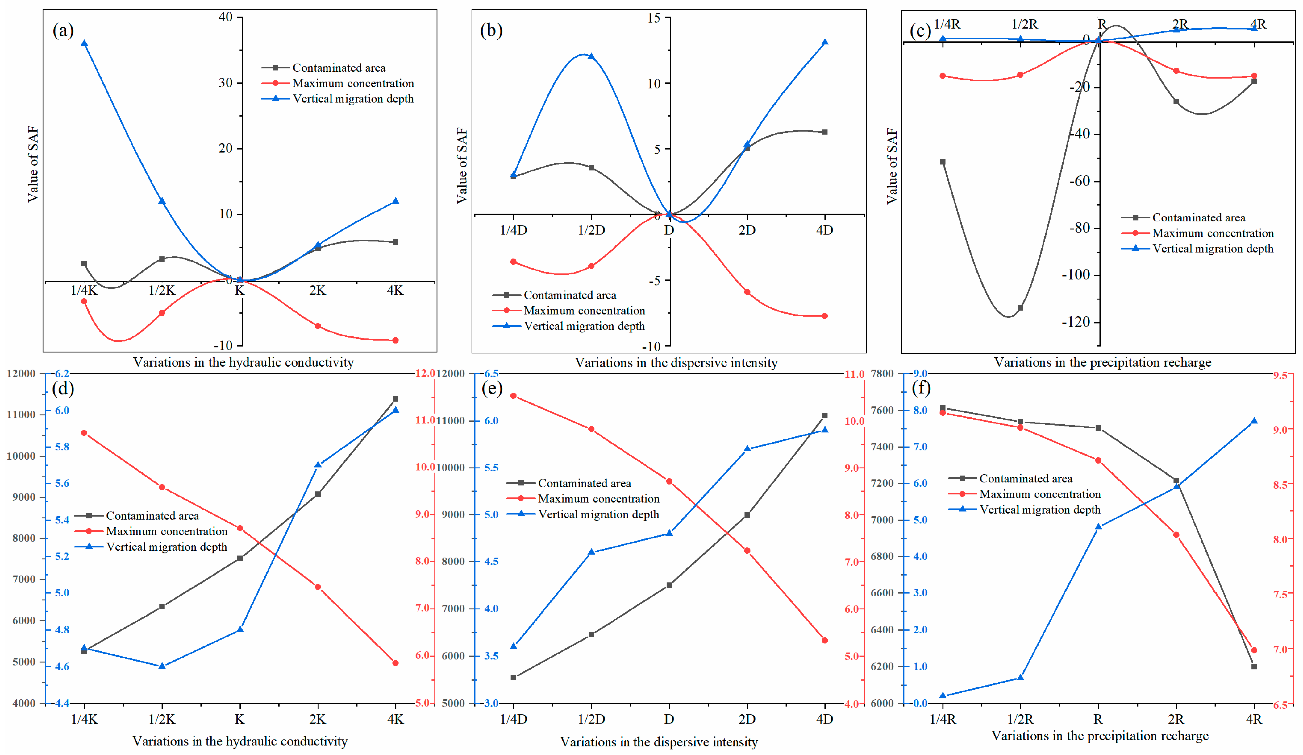
6. Results of Sensitivity Analysis

Due to the subtropical monsoon climate in the simulated area, rates of rainfall in summer are significantly higher than those in winter, and there are seasonal differences in rainfall infiltration and recharge. In addition, the Taihu plain area is mainly silty clay interbedded with thin silt, and the aquifer is composed of overlapping clay and silt with a non-uniform hydraulic conductivity. Therefore, this study investigated the influence of a single factor on pollutant migration by changing hydraulic conductivity, dispersive intensity, and precipitation recharge. First, the change value occurring during the simulation process was estimated by increasing the hydraulic conductivity, the dispersive intensity, and precipitation recharge twice and four times. Then, these estimated values were re-evaluated and reduced to a half and a quarter. For instance, (a) and (d) in Figure 9 represent the sensitivity analysis of hydraulic conductivity and the changes to the model simulation value caused by changing the hydraulic conductivity, respectively. From Figure 9a, it can be concluded that there is a positive correlation between hydraulic conductivity and pollution area and vertical migration depth within 20 years. That is, as hydraulic conductivity increases, the contaminated area and vertical migration depth of the contaminant also increase. The reason behind this phenomenon is that an increase in the hydraulic conductivity of soil results in an increase in groundwater-flow velocity, which in turn increases the contaminant migration rate along the water flow direction. This finding is supported by the study conducted by Beyabanaki [36]. Furthermore, based on SAF analysis, vertical migration depth is greatly sensitive to hydraulic conductivity, especially when hydraulic conductivity is reduced. Therefore, in soil layers with high hydraulic conductivities (such as powder soil), the vertical migration of contaminants is worthy of attention. Additionally, from Figure 9b, we can see that the sensitivity of dispersive intensity is similar to hydraulic conductivity. The relationship among precipitation recharge, horizontal contaminated area, and the vertical depth of contaminants are shown in the Figure 9c. It was discovered that there exists a negative correlation between precipitation recharge and the horizontal area of contaminant plumes. This indicates that, as precipitation recharge increases, the horizontal area of contaminant plumes decreases. Conversely, there is a positive correlation between the vertical depth of contaminants and precipitation recharge. This means that the greater the precipitation recharge, the deeper the vertical depth of contaminants. The main reason for this phenomenon is that an increase in precipitation recharge results in an increased soil porosity and water holding capacity, facilitating water infiltration and the subsequent downward movement of contaminants. This is also aided by the increase in the hydraulic conductivity of soil with the infiltration of water. Nevertheless, an enhanced hydraulic conductivity causes a reduction in the intensity of the horizontal dispersivity of contaminants, leading to a decrease in the horizontal contaminant plume area [37,38]. As a result, during the summer season with abundant precipitation, there is a heightened likelihood of contaminants migrating downwards. To mitigate the related risks, appropriate measures should be taken in pollution control and construction processes. In general, through the parameter sensitivity analysis, we can determine that the migration of groundwater pollution in this area is mainly affected by the hydraulic conductivity of soil and surface precipitation recharge [26].

7. Conclusions

Taking a decommissioned chemical plant in Suzhou as an example, this research studied the migration law and the influence range of typical chlorinated petroleum hydrocarbons (chloroform) in microconfined aquifers in the Yangtze Delta region. The specific processes of this study are as follows: (i) Based on hydrogeological data, groundwater head detection, and pumping tests of the relocated chemical plant, a numerical model for the groundwater seepage field and solute transport was established by adopting MODFLOW and the MT3DMS quantitative code in GMS software, and then the accurate groundwater flow field was obtained. (ii) The changes in chloroform concentration in microconfined aquifers over the next 20 years was successfully simulated. The results show that chloroform migrates along the direction of groundwater flow. In addition, the heterogeneity in the site also affects the development of a pollution plume. The contaminants easily migrate through soil layers with high hydraulic conductivities. In the horizontal direction, although chloroform does not migrate beyond the boundaries of the microconfined aquifer, its pollution concentration remains high within the confined area, and it is not readily biodegradable. In the vertical direction, chloroform will migrate downward to the weakly permeable layer below the microconfined aquifer, where it will be enriched but will not damage the first confined aquifer over 20 years. (iii) Based on the sensitivity analysis, hydraulic conductivity is the most sensitive parameter affecting the contaminated area, while vertical migration distance is the most sensitive to rainfall intensity.

Moreover, the numerical simulation results were analyzed and discussed, leading to the following conclusions:

(i)

In the microconfined aquifers of the Yangtze River Delta, the natural migration rate of pollutants is slow, and large-scale diffusion and migration will not occur in the short term. Therefore, during the groundwater remediation of similar pollution sites, the horizontal migration of pollutants usually does not pose a serious risk. However, to prevent the further expansion of the pollution range, corresponding anti-seepage barriers can be established according to on-site pollution monitoring results to inhibit the migration of pollutants.

(ii)

During the groundwater remediation process, soil remediation and backfilling often occur. Microconfined aquifers have a certain pressure, so attention should be paid to the secondary pollution to the upper clean soil layer caused by pollutants under capillary force and pressure. To avoid this situation, appropriate underground isolation barrier measures, such as geotextile membrane barriers and concrete wall barriers, can be taken.

(iii)

The present study’s parameter sensitivity analysis offers valuable insights into groundwater remediation. Notably, the hydraulic conductivity of soil exhibits a positive correlation with the extent of contamination and vertical migration. This finding emphasizes the importance of employing high-efficiency remediation technologies, such as activated carbon adsorption and chemical oxidation, in high hydraulic conductivity areas to effectively mitigate pollution. Conversely, in low hydraulic conductivity areas, cost-effective and practical remediation methods, such as bioremediation, may suffice. Additionally, this study highlights the fact that increased summer rainfall can worsen pollutant migration, emphasizing the importance of targeted interventions. For instance, drainage and interception facilities can be installed around the remediation site to intercept and collect precipitation and groundwater, thereby minimizing the downward migration of pollutants. Furthermore, suitable pollutant adsorbents can be incorporated into the soil to absorb pollutants and impede their downward migration.

(iv)

The research object of this paper is the microconfined aquifer of a contaminated site in the Suzhou area. This site is located in the city, and the pollution control boundary and scope are relatively clear. As the geological composition of the pollution sites in Suzhou and other areas in the Yangtze River Delta are similar to the research area, the relevant rules derived from this paper are applicable to other similar pollution sites in the Yangtze River Delta. The conclusions obtained from the calculation and simulation also have reference values for similar sites.

In summary, the research findings of this study can provide effective guidance in and a reference for the remediation and management of microconfined aquifers contaminated with chlorinated organic compounds that are similar to the study site.

References

1. Afzal, M.; Battilani, A.; Solimando, D.; Ragab, R. Improving water resources management using different irrigation strategies and water qualities: Field and modelling study. Agric. Water Manag. 2016, 176, 40–54. [Google Scholar] [CrossRef]
2. Islam, M.B.; Firoz, A.B.M.; Foglia, L.; Marandi, A.; Khan, A.R.; Schüth, C.; Ribbe, L. A regional groundwater-flow model for sustainable groundwater-resource management in the south Asian megacity of Dhaka, Bangladesh. Hydrogeol. J. 2017, 25, 617–637. [Google Scholar] [CrossRef]
3. Gleeson, T.; Befus, K.M.; Jasechko, S.; Luijendijk, E.; Cardenas, M.B. Author Correction: The global volume and distribution of modern groundwater. Nat. Geosci. 2016, 9, 161–167. [Google Scholar] [CrossRef]
4. Chen, J.; Tang, C.; Sakura, Y.; Yu, J.; Fukushima, Y. Nitrate pollution from agriculture in different hydrogeological zones of the regional groundwater flow system in the north china plain. Hydrogeol. J. 2015, 13, 481–492. [Google Scholar] [CrossRef]
5. Lapworth, D.J.; Baran, N.; Stuart, M.E.; Ward, R.S. Emerging organic contaminants in groundwater: A review of sources, fate and occurrence. Environ. Pollut. 2012, 163, 287–303. [Google Scholar] [CrossRef] [Green Version]
6. Schirmer, M.; Leschik, S.; Musolff, A. Current research in urban hydrogeology—A review. Adv. Water Resour. 2012, 51, 280–291. [Google Scholar] [CrossRef]
7. Barry, D.A.; Prommer, H.; Miller, C.T.; Engesgaard, P.; Brun, A. Modelling the fate of oxidisable organic contaminants in groundwater. Adv. Water Resour. 2002, 25, 945–983. [Google Scholar] [CrossRef] [Green Version]
8. Zhu, H.; Ye, S.J.; Wu, J.C.; Xu, H. Characteristics of soil lithology and pollutants in typical contamination sites in China. Earth Sci. Front. 2021, 28, 026–034. [Google Scholar] [CrossRef]
9. Li, H.J.; Yu, X.P.; Zhang, W.; Huan, Y.; Yu, J.; Zhang, Y. Risk Assessment of Groundwater Organic Pollution Using Hazard, Intrinsic Vulnerability, and Groundwater Value, Suzhou City in China. Expo. Health 2018, 10, 99–115. [Google Scholar] [CrossRef]
10. Yin, X.; Jiang, B.; Feng, Z.; Yao, B.; Shi, X.; Sun, Y.; Wu, J. Comprehensive evaluation of shallow groundwater quality in Central and Southern Jiangsu Province, China. Environ. Earth Sci. 2017, 76, 400. [Google Scholar] [CrossRef]
11. Zhang, Y.; Xue, Y.Q.; Wu, J.C.; Shi, X.Q.; Yu, J. Excessivegroundwater withdrawal and resultant land subsidence in the Su–Xi–Chang area, China. Environ. Earth Sci. 2010, 61, 1135–1143. [Google Scholar] [CrossRef]
12. Rahman, S.H.; Khanam, D.; Adyel, T.M.; Islam, M.S.; Ahsan, M.A.; Akbor, M.A. Assessment of Heavy Metal Contamination of Agricultural Soil around Dhaka Export Processing Zone (DEPZ), Bangladesh: Implication of Seasonal Variation and Indices. Appl. Sci. 2012, 2, 584–601. [Google Scholar] [CrossRef] [Green Version]
13. Zheng, H.R.; Cao, S.X. The challenge to sustainable development in China revealed by “death villages”. Environ. Sci. Technol. 2011, 45, 9833–9834. [Google Scholar] [CrossRef]
14. Deng, C.; Wang, S.; Li, F. Research on soil multi-media environmental pollution around a Pb-Zn mining and smelting plant in the karst area of Guangxi Zhuang Autonomous Region, Southwest China. Chin. J. Geochem. 2009, 28, 188–197. [Google Scholar] [CrossRef]
15. Hasan, M.A.; Ahmad, S.; Mohammed, T. Groundwater Contamination by Hazardous Wastes. Arab. J. Sci. Eng. 2021, 46, 4191–4212. [Google Scholar] [CrossRef]
16. Jesudhas, C.J.; Chidambaram, S.M.; Jeyakumar, R.B.; Rene, E.R. Development and application of a contaminant transport model for groundwater remediation and reservoir protection: A case study from India. Environ. Monit. Assess. 2022, 194, 257. [Google Scholar] [CrossRef]
17. Valivand, F.; Katibeh, H. Prediction of Nitrate Distribution Process in the Groundwater via 3D Modeling. Environ. Model. Assess. 2020, 25, 187–201. [Google Scholar] [CrossRef]
18. Ahmed, A.T.; Alluqmani, A.E.; Shafiquzzaman, M. Impacts of landfill leachate on groundwater quality in desert climate regions. Int. J. Environ. Sci. Technol. 2019, 16, 6753–6762. [Google Scholar] [CrossRef]
19. Gedeon, M.; Mallants, D. Sensitivity Analysis of a Combined Groundwater Flow and Solute Transport Model Using Local-Grid Refinement: A Case Study. Math. Geosci. 2012, 44, 881–899. [Google Scholar] [CrossRef]
20. Ghoraba, S.M.; Zyedan, B.A.; Rashwan, I.M.H. Solute transport modeling of the groundwater for quaternary aquifer quality management in Middle Delta, Egypt. Alex. Eng. J. 2013, 52, 197–207. [Google Scholar] [CrossRef] [Green Version]
21. Yeh, W.W.G. Review: Optimization methods for groundwater modeling and management. Hydrogeol. J. 2015, 23, 1051–1065. [Google Scholar] [CrossRef]
22. Song, S.H.; Zemansky, G. Groundwater level fluctuation in the Waimea Plains, New Zealand: Changes in a coastal aquifer within the last 30 years. Environ Earth Sci. 2013, 70, 2167–2178. [Google Scholar] [CrossRef]
23. Li, J.; Li, M.; Zhang, L. Experimental Study and Estimation of Groundwater Fluctuation and Ground Settlement due to Dewatering in a Coastal Shallow Confined Aquifer. J. Mar. Sci. Eng. 2019, 7, 58. [Google Scholar] [CrossRef] [Green Version]
24. Marchant, B.P.; McBratney, A.B.; Lark, R.M. Optimized multi-phase sampling for soil remediation surveys. Spat. Stat.-Neth. 2013, 4, 1–13. [Google Scholar] [CrossRef] [Green Version]
25. Chen, G.; Sun, Y.; Liu, J.; Lu, S.; Feng, L.; Chen, X. The effects of aquifer heterogeneity on the 3D numerical simulation of soil and groundwater contamination at a chlor-alkali site in China. Environ. Earth Sci. 2018, 77, 797. [Google Scholar] [CrossRef]
26. Shi, X.Q.; Xue, Y.Q.; Ye, S.J.; Wu, J.C.; Zhang, Y.; Yu, J. Characterization of land subsidence induced by groundwater withdrawals in Su-Xi-Chang area, China. Environ. Geol. 2007, 52, 27. [Google Scholar] [CrossRef]
27. Zhu, L.; Lu, L.; Zhang, D. Mitigation and remediation technologies for organic contaminated soils. Front. Environ. Sci. En. 2010, 4, 373–386. [Google Scholar] [CrossRef]
28. Dell’Arciprete, D.; Bersezio, R.; Felletti, F.; Giudici, M.; Comunian, A.; Renard, P. Comparison of three geostatistical methods for hydrofacies simulation: A test on alluvial sediments. Hydrogeol J. 2012, 20, 299–311. [Google Scholar] [CrossRef]
29. Dagan, G. Theory of Solute Transport by Groundwater. Annu. Rev. Fluid Mech. 1987, 19, 183–213. [Google Scholar] [CrossRef]
30. Wang, W.F.; Yua, J.; Cui, Y.; He, J.; Xue, P.; Cao, W.; Ying, H.; Gao, W.; Yan, Y.; Hu, B.; et al. Characteristics of fine particulate matter and its sources in an industrialized coastal city, ningbo, yangtze river delta, china. Atmos Res. 2018, 203, 105–117. [Google Scholar] [CrossRef]
31. Yadav, N.; Yadav, A.; Kim, J.H. Numerical solution of unsteady advection dispersion equation arising in contaminant transport through porous media using neural networks. Comput. Math. Appl. 2016, 72, 1021–1030. [Google Scholar] [CrossRef]
32. Doherty, J. PEST: Model Independent Parameter Estimation. In User Manual, 5th ed.; Elsevier: Amsterdam, The Netherlands, 2004. [Google Scholar] [CrossRef]
33. González, C.H.; Fraguela, B.B.; Andrade, D.; García, J.A.; Castro, M.J. Numerical simulation of pollutant transport in a shallow-water system on the Cell heterogeneous processor. J. Supercomput. 2013, 65, 1089–1103. [Google Scholar] [CrossRef]
34. Banaei, S.M.A.; Javid, A.H.; Hassani, A.H. Numerical simulation of groundwater contaminant transport in porous media. Int. J. Environ. Sci. Technol. 2021, 18, 151–162. [Google Scholar] [CrossRef]
35. Agarwal, P.; Sharma, P.K. Analysis of critical parameters of flow and solute transport in porous media. Water Supply 2020, 20, 3449–3463. [Google Scholar] [CrossRef]
36. Beyabanaki, S.A.R.; Bagtzoglou, A.C.; Anagnostou, E.N. Effects of groundwater table position, soil strength properties and rainfall on instability of earthquake-triggered landslides. Environ. Earth. Sci. 2016, 75, 358. [Google Scholar] [CrossRef]
37. Johnson, R.L.; Thoms, R.B.; Zogorski, J.S. Effects of daily precipitation and evapotranspiration patterns on flow and VOC transport to groundwater along a watershed flow path. Environ. Sci. Technol. 2003, 37, 4944–4954. [Google Scholar] [CrossRef]
38. Bahar, T.; Oxarango, L.; Castebrunet, H. 3D modelling of solute transport and mixing during managed aquifer recharge with an infiltration basin. J. Contam. Hydrol. 2020, 237, 103758. [Google Scholar] [CrossRef]
Figure 1. Location of the study area in the city of Suzhou, southeast of the Jiangsu Province of China.
Water 15 01381 g001
Figure 2. Hydrogeological cross section of study area.
Water 15 01381 g002
Figure 3. Workflow chart for numerical simulation research.
Water 15 01381 g003
Figure 4. Generalization and setting of model boundary conditions.
Water 15 01381 g004
Figure 5. Groundwater levels of the study site; (a) contour of the simulated and observed water heads of the microconfined aquifer; and (b) the comparison between the computed and observed values.
Water 15 01381 g005
Figure 6. Contour map of chloroform concentration in the study area.
Water 15 01381 g006
Figure 7. Simulation of pollutant concentration and prediction of concentrations at (a) 50 d, (b) 1850 d, (c) 3650 d, and (d) 7300 d, and the distribution of hydraulic conductivity in the microconfined aquifer.
Water 15 01381 g007
Figure 8. The adjacent soil layer of the microconfined aquifer and the transport status of contaminants in the first confined aquifer predicted over the next 20 years; (a) Pollutant migration for 50 days; (b) Pollutant migration for 1850 days; (c) Pollutant migration for 3650 days; (d) Pollutant migration for 7300 days.
Water 15 01381 g008
Figure 9. (a) Sensitivity analysis of the hydraulic conductivity, (b) dispersive intensity, and (c) precipitation recharge in the transport model, and the values of the contaminated area, maximum concentration, and vertical migration depth when (d) the hydraulic conductivity, (e) dispersive intensity, and (f) precipitation recharge are changed.
Water 15 01381 g009