Article

Extraction and Classification of Flood-Affected Areas Based on MRF and Deep Learning

1
School of Civil Engineering, Sun Yat-Sen University, Guangzhou 510275, China
2
Guangdong Research Institute of Water Resources and Hydropower, Guangzhou 510635, China
*
Author to whom correspondence should be addressed.
Water 2023, 15(7), 1288; https://doi.org/10.3390/w15071288
Submission received: 15 February 2023 / Revised: 15 March 2023 / Accepted: 21 March 2023 / Published: 24 March 2023

Abstract

:
Floods can cause huge damage to society, the economy, and the environment. As a result, it is vital to determine the extent and type of land cover in flooded areas quickly and accurately in order to facilitate disaster relief and mitigation efforts. Synthetic aperture radar (SAR) is an all-weather, 24 h data source used to extract information about flood inundations, and its primary aim is to extract water body information for flood monitoring. In this study, we have studied the backscattering characteristics of water and non-water, combined the threshold segmentation method with Markov random fields (MRF), and embedded simulated annealing (SA) in the process of image noise reduction, resulting in the development of a water extraction method KI-MRF-SA with high accuracy in classification and high automation. Furthermore, object-scale adaptive convolutional neural networks (OSA-CNN) are introduced for the classification of optical images before the flood in order to provide reference data for flood inundation analysis. The method proposed in this study consists of the following three steps: (1) The Kittler and Illingworth (KI) thresholding algorithm is used for the segmentation of SAR images in order to determine the initial flood inundation extent; (2) MRF and SA algorithms are employed as a means to optimize the initial flood inundation extent, and the results are combined across multiple polarizations by using an intersection operation to determine the final flood inundation extent; and (3) As part of the flood mapping process, land cover types before the flood are classified using OSA-CNN and combined with flood inundation extents. According to the experimental results, it is evident that the proposed KI-MRF-SA method is capable of distinguishing water from non-water with significantly higher accuracy (3–5% improvement in the overall accuracy) than conventional thresholding methods. Combined with the classification method of OSA-CNN proposed in our earlier research, the overall classification accuracy of flood-affected areas could reach 92.7%.

1. Introduction

As one of the most devastating natural disasters in the world, floods cause a large number of casualties and economic losses every year due to their sudden occurrence, wide range of influence, and high recurrence rate [1,2,3,4,5]. Accordingly, as flood risks increase, timely and synoptic observations of flood water extents are essential in order to respond to and manage disasters efficiently [6,7].
Optical remote sensing images are one of the most commonly used data sources for land use classification. However, since the visible and near-infrared spectrums of the optical sensor have weak penetration ability, which makes it more susceptible to extreme weather conditions, and because floods are often accompanied by extreme weather events such as cloudy and rainy weather, a large number of non-detection zones may occur as a result. As an active detector, SAR is well suited for flood mapping since it is capable of providing 24 h observations regardless of adverse lighting or weather conditions. Thus, it can also compensate for certain shortcomings of optical remote images [8,9,10,11].
Floods are caused by water flooding; thus, the key to utilizing SAR as a means to monitor floods lies in the detection and mapping of water bodies. The backscattering intensity of a SAR image is closely related to the ground’s surface roughness. Water bodies have smooth surfaces that typically reflect the radar signal in the specular direction away from the antenna, thereby producing a very low backscattering effect [9,12]. In the case of study areas with flooding, the histogram of SAR images usually exhibits a bimodal distribution, with one peak corresponding to water and another to non-water areas [13,14,15]. Accordingly, since the water extraction method based on thresholding segmentation is simple and efficient, it has been widely applied in a large number of studies [16,17,18,19,20,21,22]. In recent years, in spite of the substantial advances in flood mapping with SAR, further research is still needed in order to detect flood inundation in complex environments such as vegetation and urban areas [23,24,25,26,27,28,29], because radar signals may be quite complex and difficult to predict in these places. Smooth land surfaces may exhibit specular scattering [30,31,32], but extreme weather conditions, such as heavy precipitation and strong storms may cause rough water surfaces, which reduce the backscattering contrast between water and non-water surfaces [33]. Consequently, a large amount of noise may appear in the image after thresholding segmentation, which may disturb the classification accuracy.
In this study, we aim to fully exploit the potential of SAR images for the detection of water bodies, to correlate water and non-water areas in spatial distribution, and to present a technical framework for “extraction and refinement” through the use of context information. Firstly, a water body is extracted through thresholding segmentation and binarization. This step is designed to quickly determine the initial water extent, which may involve a number of noise errors as well. Secondly, on the basis of the binary image, the neighborhood relationship of pixels is fully taken into consideration, and MRF is then utilized to denoise the image. Furthermore, the simulated annealing (SA) method is incorporated in the iterative process in order to achieving the global optimum in the denoising process by preserving image detail while reducing noise errors, thereby facilitating the rapid extraction of the flood inundation extent. In comparison to the conventional threshold method, the proposed method minimizes the interference of speckle noise on the image. The conventional threshold pursues an optimal threshold, which is used for the simple division of water and non-water. Nevertheless, speckle noise causes their backscattering histograms to overlap, and a single threshold cannot distinguish between water and non-water. In contrast, the proposed method does not excessively rely on the selection of a threshold but rather adopts post-processing to eliminate commission and omission errors. This yields a globally optimal solution for water extraction, which considerably enhances the accuracy of water identification.
On the basis of the identification of flood inundation extent, we expect to obtain the land cover types through optical image classification, which can provide data support for further inundation analysis. Traditionally, land cover type classification methods operated at the pixel level and assessed the geometrical, textural, and contextual features surrounding the focal pixels. The problem is that the land-surface information presented by optical remote sensing images is complex, with fuzzy and uncertain semantics, and pixel-based classification often suffers from errors in scale, morphology, or attribute. Compared with traditional classification methods, deep learning technology can automatically learn image features from massive images, avoid manual feature extraction, and achieve high accuracy in image classification. Deep learning-based image classifications that utilize convolutional neural networks (CNNs) are research hotspots in the field of remote sensing image processing [34,35,36]. Typical applications include scene classification [37,38,39,40,41,42] and land use/land cover classification [43,44,45,46]. However, CNN requires fixed inputs of object primitives, without considering multiple scales of different objects. In order to solve this problem, the object-scale adaptive convolutional neural networks (OSA-CNN) method was proposed in our previous study and successfully applied to the classification of optical remote sensing images [47]. The method combines object-based image analysis (OBIA) with CNN, in which multi-scale image segmentation and CNN classification are combined through an object-scale adaptive mechanism and achieve high image classification accuracy. In the current study, we also adopted this method in order to determine the land cover types before the flood, thereby providing a data reference for the flood inundation analysis.
The remainder of this article is organized as follows: Section 2 introduces the remote sensing images and the study sites; Section 3 introduces the details of the proposed method, including the major components and the validation design; Section 4 conducts an experimental analysis and accuracy evaluation; Section 5 discusses the proposed method and key parameters; and Section 6 provides concluding comments.

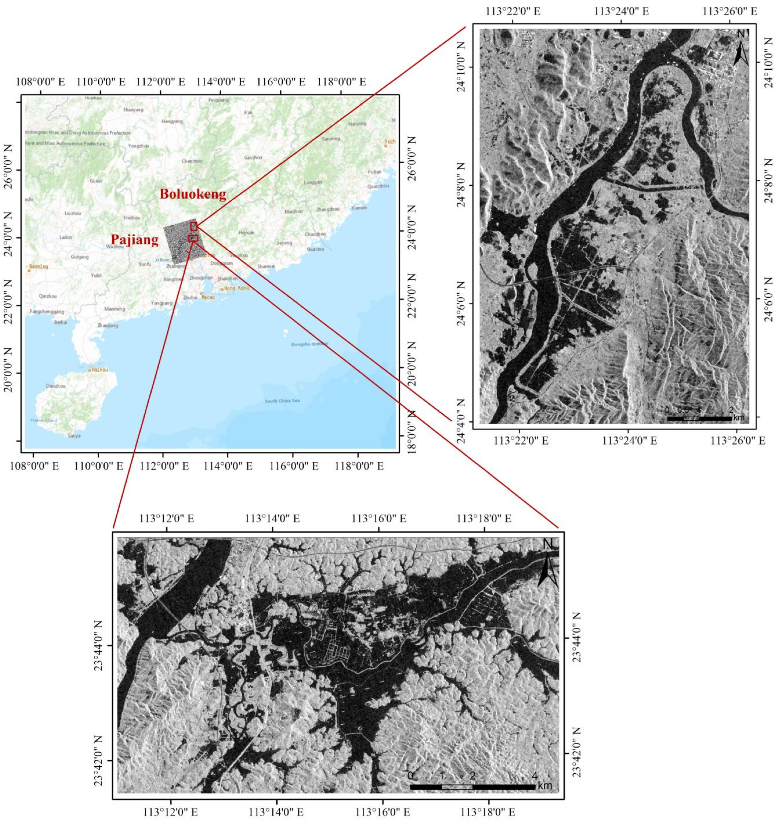
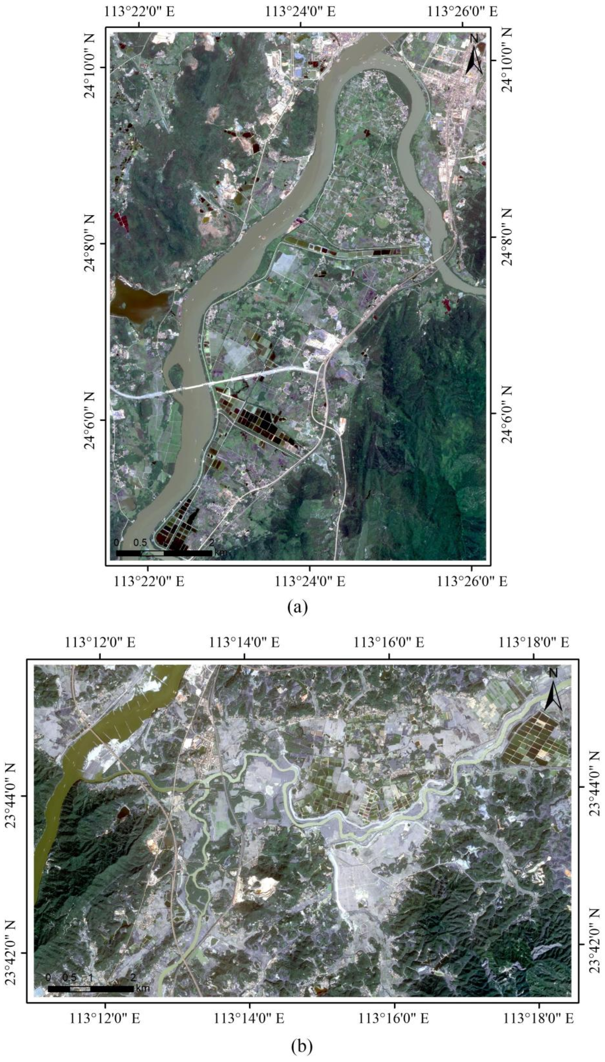
2. Test Case and Dataset
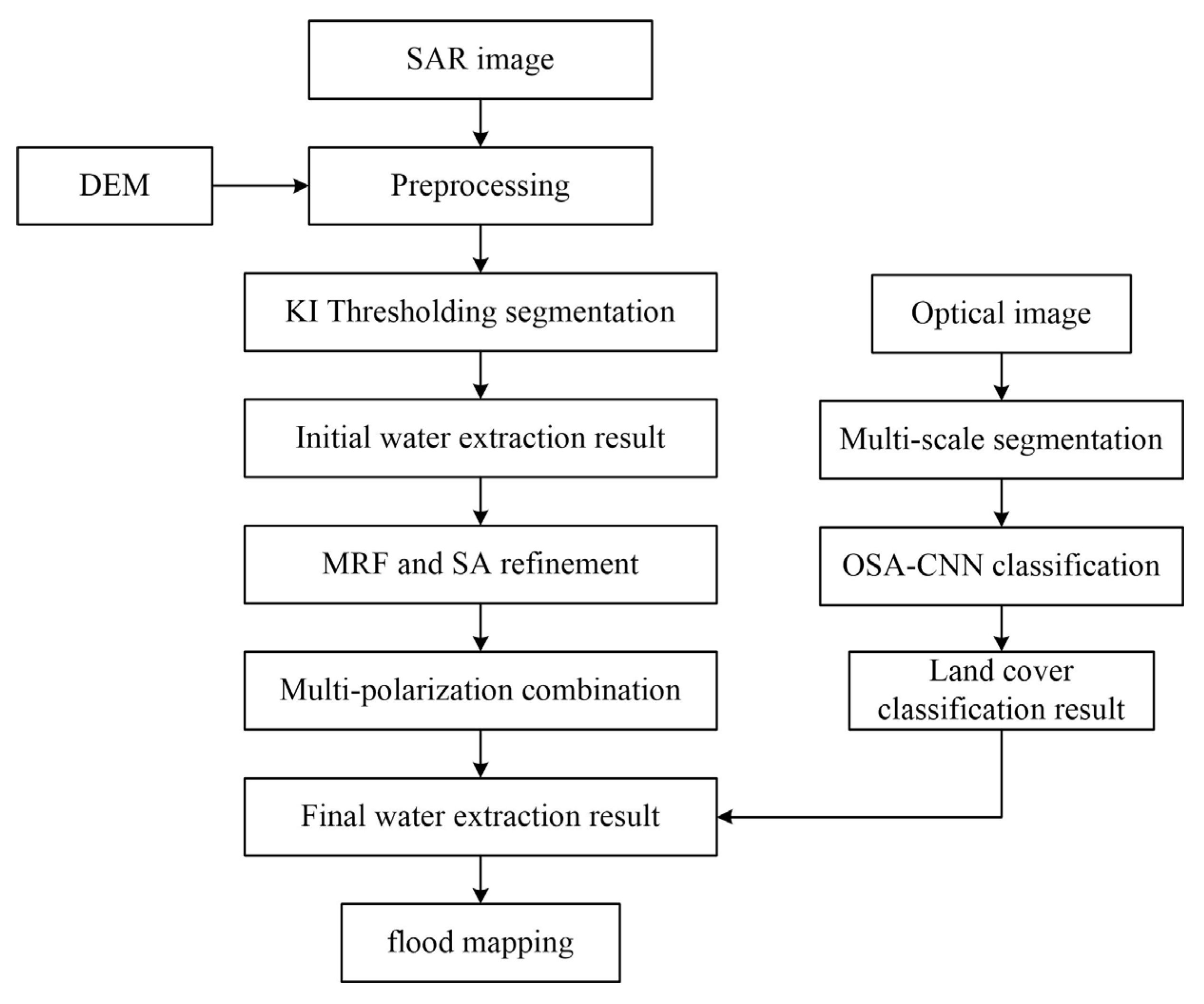
From June 12 to 25, 2022, the Pearl River Basin experienced heavy rainfall for seven consecutive days, causing a wide range of catastrophic floods. The floods affected 102 villages in five provinces, including an area of 113,070 hectares of croplands, 239,500 people who were relocated, and a direct economic loss of RMB 11.652 billion. Among the flood locations, Yingde City and Qingyuan City were the most severely affected. Our research was conducted on the flood-affected areas of Boluokeng and Pajiang in these two cities and collected the GF-3 images of the two experimental areas on 24 June 2022. At the time, the flooding was still ongoing and close to its peak. In addition, we have also collected the GF-2 data images before the event in order to analyze the land cover types before the flood, as shown in Table 1.
During the flood, the China Centre for Resources Satellite Data and Application gathered a large amount of data in this area (as part of the national response to sudden natural disasters), and the GF-3 used in this research is the only microwave remote sensing satellite in the major projects of the “China High-Resolution Earth Observation System,” as well as China’s first multi-polarization high-resolution synthetic aperture radar satellite. The GF-3 SAR data used in this study are dual-polarization (VV, VH) images acquired in Fine Stripe 2 (FSII) mode. According to the spatial resolution reports, it is evident that the sensor is capable of effectively identifying adjacent targets with an azimuth of 8 to 12 m and a range of 10 m; thus, the image resolution was set to 10 × 10 m during preprocessing. Upon completing the preprocessing, the sizes of the intercepted test areas were 1045 × 1411, and 2033 × 1319, respectively, and the coverage area was as shown in Figure 1, with the HV polarimetric SAR image as the base map.
During a flood event, it is not easy to obtain reliable and high-quality optical remote images of an area depicting the environment. It should be noted that floods are often accompanied by cloudy and rainy weather. Extreme weather hinders the acquisition of surface information by optical sensors, and many optical remote images with clouds cannot be directly used. Given the width of high-resolution optical satellites is smaller than that of SAR satellites, and the revisiting time is relatively long, a comprehensive and quantitative large-scale comparison between optical satellite images and SAR data is difficult to carry out. As a result, we have collected as much information as possible from multiple data sources, and selected typical areas among them for carrying out a local comparison by employing SAR data as they became available. Finally, we have selected the GF-2 optical satellite, which is the civil remote sensing satellite with the highest spatial resolution independently developed by China to date. The GF-2 optical satellite is equipped with a multi-spectral camera with a resolution of 4 m, and it also possesses effective earth observation capabilities. The image data we collected were taken on 11 November 2021, about 6 months before the flood, and the types of land coverage showed little change. At the time, there were few clouds in the sky, and the conditions for remote sensing shootings were favorable, making it possible to easily classify land coverage types. The GF-2 data collected at the time basically overlap with the SAR data range and cover the flood-affected area. The image sizes of the two test areas are 1972 × 2768 and 3160 × 1953, respectively, and the coverage area is shown in Figure 2.

3. Methodology

In this study, the main technical process of the method proposed is shown in Figure 3, which is mainly divided into the following two modules: (1) The KI-MRF-SA method is used to delineate the flood water extent based on SAR images in the event of a flood. The primary implementation steps of this module include: firstly, the SAR data are preprocessed through the Environment for Visualizing Images (ENVI) 5.6.2 software; then, the initial extent of the water body is delineated by employing the Kittler and Illingworth (KI) thresholding algorithm; finally, MRF and SA are used as a means to refine the extraction results, and the final flood water extraction results are obtained through multi-polarization fusion. (2) The OSA-CNN method is employed for the classification of optical remote sensing images before the occurrence of the flood. In order to obtain the entire image classification result, multi-scale image segmentation is conducted along with CNN classification and multi-scale classification fusion. Upon completing the above two steps, the water body extraction results and the land cover classification results are superimposed in order to determine the land types within the flood-affected areas.

3.1. Image Preprocessing

The SAR data of this study were preprocessed by employing the SARscape module of ESRI’s commercial software, ENVI 5.6.2. The original data of GF-3 employ two bands in order to store the real part and the imaginary part in one file, which is then imported into SARscape and automatically combined into Single Look Complex (SLC) data. Subsequently, the following preprocessing steps were applied to each image: multi-looking, terrain correction using a DEM, radiometric calibration, and geocoding. Firstly, the SAR intensity images were generated from the SLC image according to the range and azimuth looks, which were automatically determined due to the geometric relationship between the incident angle and the range and azimuth directions in multi-looking. In the process of geometric correction, the elevation data were downloaded from the National Elevation Dataset with a resolution of 5 m. There is also an automatic download DEM feature available through SARscape, including the 30-m and 90-m grids of NASA’s Shuttle Radar Topography Mission (SRTM). The refined Lee speckle filter was applied in order to reduce the noise level of the intensity images, following which, the images were geocoded and resampled to the SAR orthophotomap with a resolution of 10 m. In the automatic preprocessing process, the majority of the default parameter settings of SARscape for GF3 data were adopted, except for the output image resolution, to ensure accurate data processing efficiency with minimal manual participation.
Since the downloaded GF-2 image is at the L1A level and has been radiometrically corrected, it can only be used directly after it has been orthorectified. Through overlay analysis, it was found that the spatial positions of the GF-2 and GF-3 images do not precisely match, resulting in several pixels of deviation between them. In this study, the GF-2 image obtained after orthorectification was utilized as a reference image, and the GF-3 SAR image was matched with the GF-2 image by making use of coordinate translation.

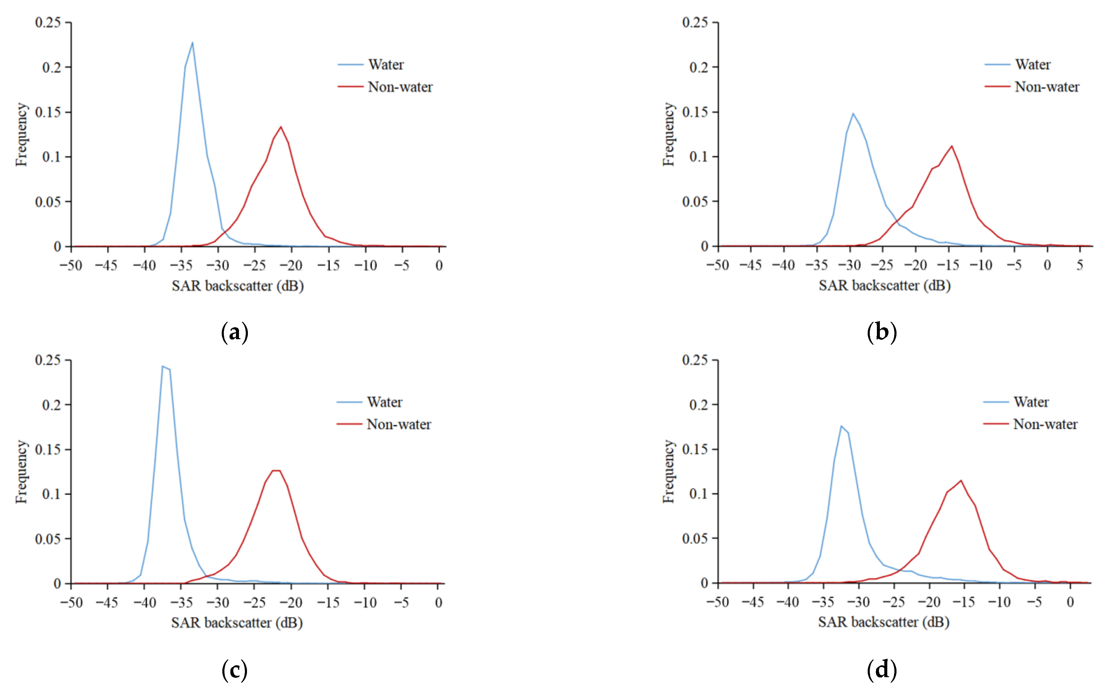
3.2. Thresholding Segmentation

There is a close relationship between the intensity of backscattering and the roughness of the ground surface. There is a low backscattering intensity in water bodies due to their smooth surfaces, as opposed to vegetation, bare land, and towns, which have a rough surface, resulting in a high backscattering intensity. Therefore, the threshold-based method is simpler and more efficient as a means for distinguishing water and non-water areas in images. In particular, backscattering values below a candidate threshold represent water pixels, and the rest represent non-water. A smaller threshold usually identifies water extent with higher confidence, while a larger threshold tends to increase the confidence of non-water [15]. In this study, some regions of interest from GF-3 images in FSII mode were selected for analysis of their optimal thresholds. The water pixels represent areas including rivers, lakes, ponds, and flood-affected areas, and the non-water pixels represent areas including cropland, construction land, woodland, bare soil, etc., with a total of 20,000 pixels. The backscattering ranges of the water and non-water areas of the HH and HV polarizations have been calculated separately, and the histograms of the two polarization images are shown in Figure 4.
According to Figure 4, it is evident that the backscattering intensity of the water areas in the two experimental areas is significantly smaller than that of the non-water areas, and they are partially overlapped. Thresholding is greatly influenced by how much overlap there is between two distributions of water and non-water areas.
As compared with HH polarization, HV polarization has a smaller histogram overlap area between water and non-water areas, making it relatively easier to distinguish between them. This is due to the fact that the cross-polarized image information is mainly determined by volume scattering and is less sensitive to specular scattering. In addition, the surface of the water is smooth and uniform, and the noise level in the cross-polarized image is lower, which is more conducive to the detection of water bodies.
Through visually interpreting the probability density curves of the SAR image of Boluokeng, it is possible to achieve more favorable water identification results by employing −29 dB and −23 dB as the segmentation thresholds of HV polarization and HH polarization, respectively; the optimal segmentation thresholds of Pajiang are −32 dB and −24 dB, respectively.
By employing the backscattering intensity of a selected sample, the visual interpretation method summarizes the distribution range of water bodies in the image. Researchers have utilized this method quite extensively. However, the acquisition of the threshold depends on manual analysis and summary, which may involve a certain degree of subjectivity. In addition, manual participation in judgment reduces its efficiency. Thus, an automatic threshold selection method is necessary in this case. In this study, Otsu’s and KI’s thresholding segmentation methods are employed for image binarization, and the results are then compared in order to prove their effectiveness.
As an early-developed image segmentation method, Otsu’s method maximizes the variance between two classes in order to determine a threshold [48]. We define the segmentation threshold as T, the proportions of the number of pixels in the two categories as ω 0 and ω 1 , and the corresponding mean values as μ 0 and μ 1 , respectively. The inter-class variance σ B can be calculated according to the following function:
σ B 2 = ω 0 ( μ 0 μ ) 2 + ω 1 ( μ 1 μ ) 2 = ω 0 ω 1 ( μ 0 μ 1 ) 2
The selection of a suitable threshold T is based on the maximum of a given predefined function.
Although a SAR image intensity histogram does not completely conform to the Gaussian distribution, the Gaussian distribution results in a better fitting effect as compared to other existing empirical statistical models. In this study, the KI’s thresholding algorithm [49] has been adopted, which is predominantly used in remote sensing image analysis [50,51,52,53]. In this technique, the sets of pixels in grayscale images are grouped into object and background classes using the minimum error approach. The fitting criterion function under the Gaussian distribution is defined as:
J ( T ) = 1 + 2 [ P w ( T ) l n σ w ( T ) + P n ( T ) l n σ n ( T ) ] + 2 H ( Ω , T )
H ( Ω , T ) = 2 [ P w ( T ) l n P w ( T ) + P n ( T ) l n P n ( T ) ]
where P w ( T ) and P n ( T ) represent the prior probability of water and non-water areas at the threshold T, and σ w ( T ) and σ n ( T ) are the corresponding standard deviations. As long as the threshold T is varied, the models of the Gaussian distributions change. The lower the value of the criterion function, the better the model fits the data.

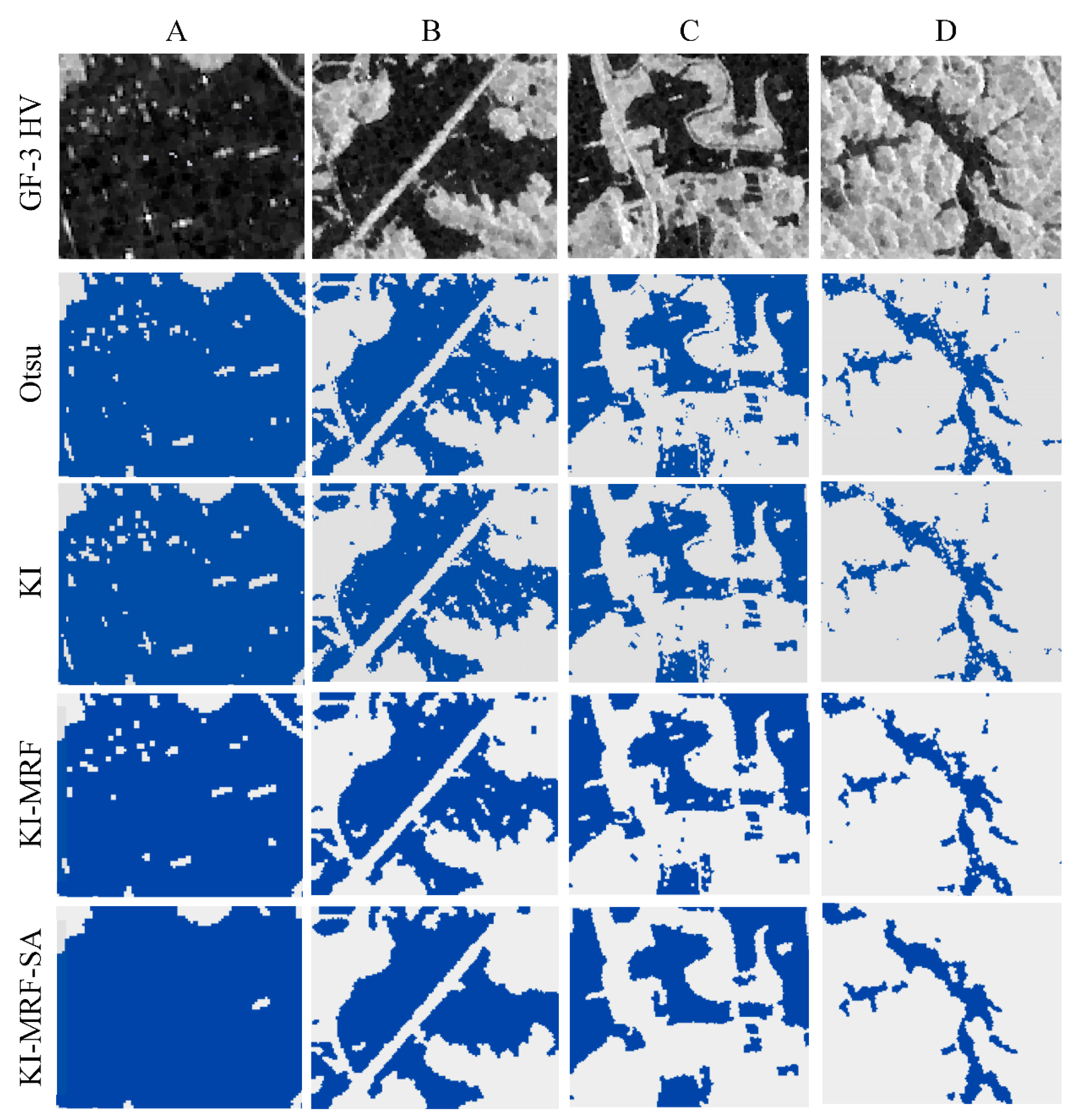
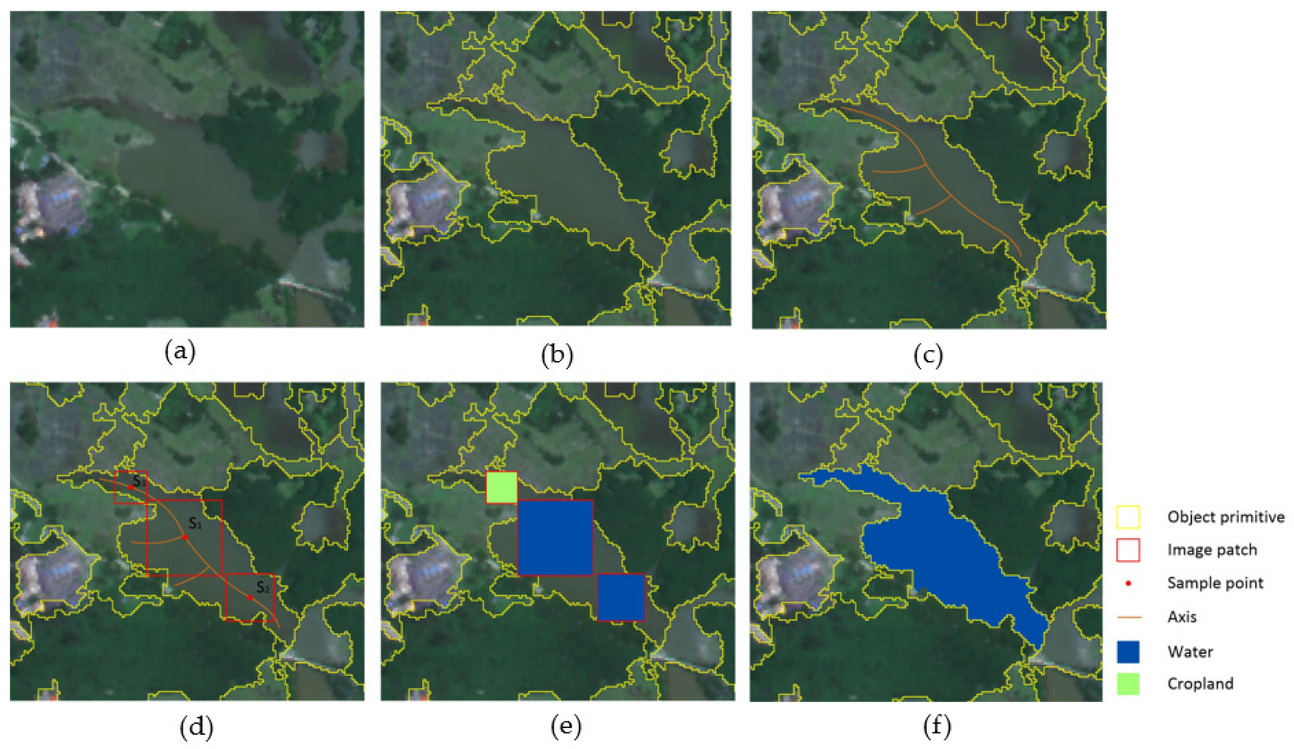
3.3. Refinement of the Water Extraction Method

Otsu’s and KI’s thresholding segmentation methods are only capable of turning all the pixels of an image into one-dimensional samples for unsupervised classification; however, these methods do not take the spatial neighborhood information into consideration, and are vulnerable to noise in complex environments. Although the noise level of SAR images can be reduced through multi-look, filtering, and other processes during preprocessing, there are a number of inherent speckle noises with high scattering that are difficult to eliminate. Furthermore, excessive filtering may lead to the degradation of the image resolution and may exhibit water bodies with blurred edges, resulting in a decrease in the final classification accuracy. Accordingly, it is necessary to employ methods that involve both noise suppression as well as detail preservation in order to perform more accurate classification of a SAR image.
MRF is capable of fully utilizing context information and prior knowledge of image features, and can accurately describe the dependencies between pixels. In this study, MRF is adopted in order to extract water bodies more accurately. First, the SAR image is converted into a binary image through threshold segmentation, with the water pixels marked as 1 and the non-water pixels marked as −1. x i is defined as the pixel from the original image, and y i as the pixel in the observed image. The process of removing noise can be regarded as the process of restoring the random field y to the real random field x. Generally, the pixels in the original image are closely related to those in the observed image, and each pixel is relatively close to its surrounding pixels since there is no noise in the original image. The following prior knowledge can be obtained: 1. x i is related to y i ; 2. x i is only related to its adjacent pixel x j from the original image. Thus, the complex Markov model can be divided into a series of simple cliques composed of { x i , y i , x j } , and the energy function is defined as:
E ( x , y ) = h i x i β { i ,   j } x i x j η i x i y i
The corresponding joint probability distribution function is as follows:
P ( x ,   y ) = 1 Z e x p { E ( x , y ) }
where h ,   β ,   and   η represent the non-negative weight, and Z represents the normalization factor. In conclusion, the lower the energy, the higher the joint probability distribution, and in turn, the denoised image has a higher probability of being consistent with the original image.
The optimization of the solution is carried out by employing the Iterated Conditional Modes (ICM) strategy [54]. This strategy calculates local energy changes by changing the current pixel and fixing other pixels in each iteration, and it provides the advantages of convenient calculation, eliminates the need to repeat the calculation of global energy, and is highly efficient. However, it also has certain defects, which may lead to relatively dense noise points forming noise blocks, thus falling into a local optimum. In order to obtain a better denoising result, it is necessary to adopt a strategy that can lead to obtaining the global optimum. The simulated annealing method [55] is a recursive and iterative global optimization algorithm that is capable of randomly searching for the global optimal solution by accepting the local non-optimal solution with a certain degree of probability. The key to simulated annealing is finding an acceptably good solution by calculating the acceptable probability q based on the current temperature t, and determining whether or not the current change should be accepted based on the Metropolis acceptance criteria [56]. The specific algorithm flow is as follows:
Step 1: Threshold segmentation is performed for each polarization of a SAR image, and the water pixels and non-water pixels are initialized to 1 and –1, respectively;
Step 2: The current temperature t is calculated based on the current iteration number k and the maximum iteration number kmax;
Step 3: Each pixel x k is traversed and converted into {1 and −1} in order to calculate the local energy change Δ E ;
Step 4: The acceptable probability q is calculated based on Δ E and t, and the current pixel value is modified to x k + 1 according to the Metropolis acceptance criterion;
Step 5: Steps 2–4 are then repeated until the maximum number of iterations is reached or the difference between the two adjacent global energy changes is less than 0.1%;
Step 6: Based on the results of the water extraction process in different polarization images, the final result is generated through the operation of intersection.
During the algorithm process, the cooling schedule controls the entire algorithm flow. The temperature in the cooling schedule does not necessarily have any actual physical meaning, but as the iterative calculation proceeds, the temperature should gradually approach zero. Thereby, the result can converge to the global optimal. In this study, the temperature calculation formula was designed as:
t ( k ) = s ( 1 k 1 k m a x )
where s is a constant for controlling the rate of temperature drop, and k and kmax are the current iteration number and the maximum iteration number. In this study, s was set at 0.01, and kmax was set at 30.
x k is defined as the value of pixel x in the kth iteration, E ( x k ) refers to the local energy only affected by x k , and E ( x n e w ) refers to the new local energy after changing the value of x k . Based on the current temperature t and the local energy change, the acceptable probability q can be calculated using the following formula:
q = e x p ( E ( x n e w ) E ( x k ) t )
Subsequently, the change of the current pixel is accepted probabilistically according to the Metropolis criterion:
x k + 1 = { x n e w ,   q 1   o r   q > ξ x k , q < ξ
where ξ is a random number uniformly distributed on the [0, 1] interval. When q is greater than ξ or q is greater than or equal to 1, the current pixel change is accepted; otherwise, it is not accepted. In each iteration of ICM and SA, the water distribution map is continuously updated. When the global energy change between two adjacent iterations is less than 0.1% or the number of iterations reaches 30, the iteration is terminated and the flood inundation map is generated accordingly.
As SAR images are usually composed of multiple polarizations, multiple polarizations can be combined in order to take advantage of more information about the land surface, thereby improving the delineation of water bodies. Consequently, we first delineated the flood inundation map at each polarization and then applied an intersection operation in order to combine flood inundation maps across the various polarizations (i.e., a pixel is labeled as water only if it appears in different polarizations).
This method does not only integrate the multi-polarization data of the SAR image, but also takes into account the global optimization of the noise reduction process. By enhancing its ability to suppress the inherent speckle noise and maintain the detailed quality of the images, the robustness of the method is enhanced.

3.4. Classification of Flooded Area

In our previous research, we have proposed the OSA-CNN classification method [47], and demonstrated the effectiveness of this method in the classification of optical remote images. OSA-CNN is divided into two main modules. The first one is the image segmentation and classification module. The object primitives at a set of scales are obtained through hard-boundary-constrained segmentation (HBC-SEG) [57,58,59,60,61]. Then, the object primitives are mapped into image patches using adaptive patch sampling along the object primitive axes, and the results are classified using CNN. These processes are conducted at all scales to obtain a set of classification results. The second one is the multiscale classification fusion module. Each object primitive is classified through majority voting on the image patches’ classification results to obtain the entire image classification result. The object primitive/image patch conversion, CNN network modification, and multiscale classification fusion are the key links for fulfilling the proposed method. In the current study, this method is employed as a means to carry out the classification of land cover types before the occurrence of floods. In addition, two scales of 50 and 100 are utilized for segmentation according to the specific conditions of the two experimental areas, and the OSA-CNN model is used to distinguish between the five main land cover types: water, woodland, cropland, bare soil, and construction land.
The implementation process of the model is depicted in Figure 5. First, HBC-SEG is utilized for image segmentation to convert the image into a series of object primitives, as demonstrated in Figure 5b. Second, the axis of each object primitive is extracted to obtain the sampling candidate points, as illustrated in Figure 5c. Third, the object primitives are mapped into image patches using adaptive patch sampling along the object primitive axes, as shown in Figure 5d. Finally, OSA-CNN is employed for the classification of each image patch. The object primitive classification results are achieved through voting, as depicted in Figure 5e,f. Figure 5 is the OSA-CNN classification process at one scale. The image patches at more scales can be obtained through multi-scale segmentation, and the classification results at different scales will be considered in the voting process.
The adaptive patch sampling scheme is as follows:
Step 1: Position the first image patch sample at the widest axis point and set the square width to double the axis width (e.g., S1 in Figure 5d);
Step 2: Excluding the axes covered by the sample generated in Step 1, search the remaining axes for the second widest axis point and generate the candidate sample. Discard the candidate if its overlap rate with prior samples exceeds 30%; otherwise, consider the candidate as a new image patch sample (e.g., S2 in Figure 5d);
Step 3: Repeat Step 2 until no axis points are available or until the number of samples reaches a certain threshold.
These image patches cover the majority of the parts of the object primitive, accurately represent the object primitive’s configuration, and facilitate the subsequent CNN training and classification. For OSA-CNN network structure and other details, refer to [47].
The surface water is extracted from the images before and after the flood inundation, and the water and non-water pixels are assigned as 1 and 0, respectively, in order to obtain binary images. Then, the binary images are superimposed for change detection, and the flood inundation extent is obtained through the following formulas:
Δ P = P 2 P 1
W = { 1 ,     Δ P > 0 0 ,     Δ P 0
where P 1 and P 2 refer to the binary images before and after the flood inundation, respectively. W = 1 refers to the flooded pixels, and W = 0 refers to the non-flooded pixels. By superimposing the flood inundation extent and the land cover types before the occurrence of the flood, the flood inundation map can be obtained.

3.5. Accuracy Evaluation
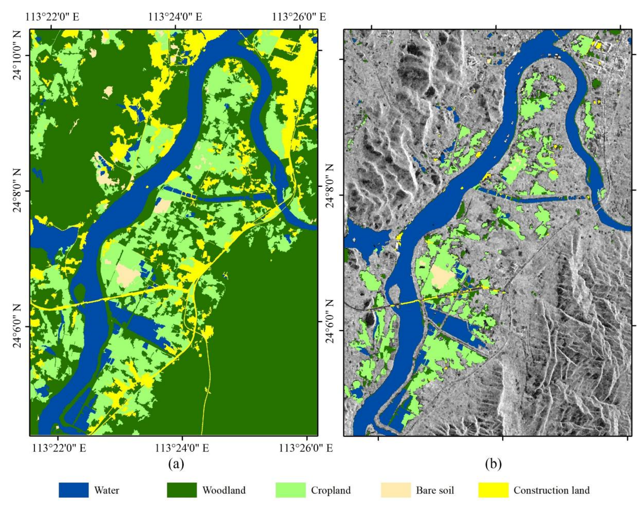
A confusion matrix was established to evaluate the accuracy of the compared methods. The accuracy measures used in this study include user accuracy (UA), producer accuracy (PA), overall accuracy (OA), and Kappa.
U A ( a ) = X a a i = 1 n X a i
P A ( a ) = X a a i = 1 n X i a
O A = i = 1 n X i i N
K a p p a = N a = 1 n X a a a = 1 n ( i = 1 n X a i × i = 1 n X i a ) N 2 i = 1 n ( i = 1 n X a i × i = 1 n X i a )
where n represents the number of classes, N denotes the total number of test samples, and X a i represents the number of samples whose actual and predicted classes are a and i, respectively.

4. Results

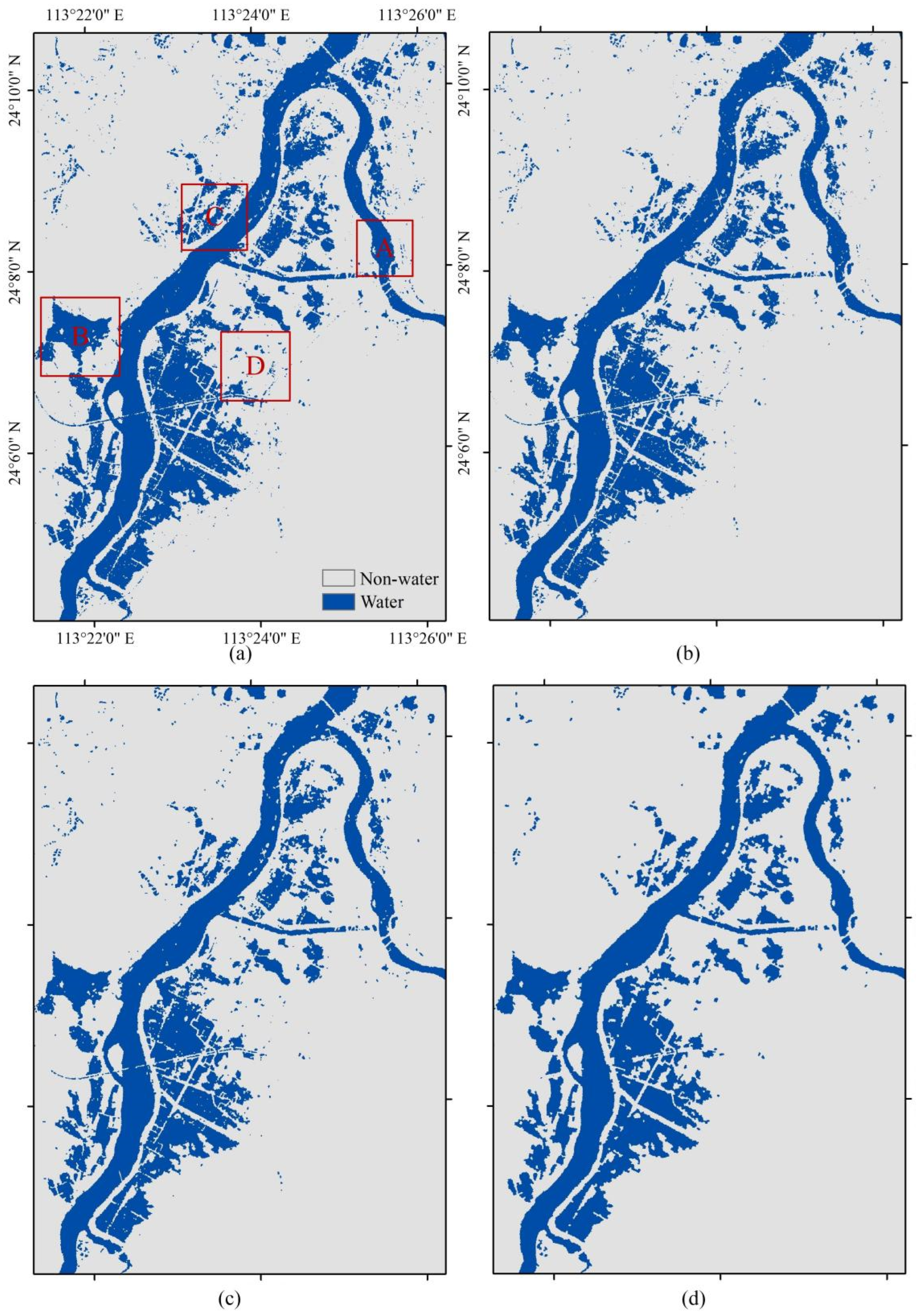
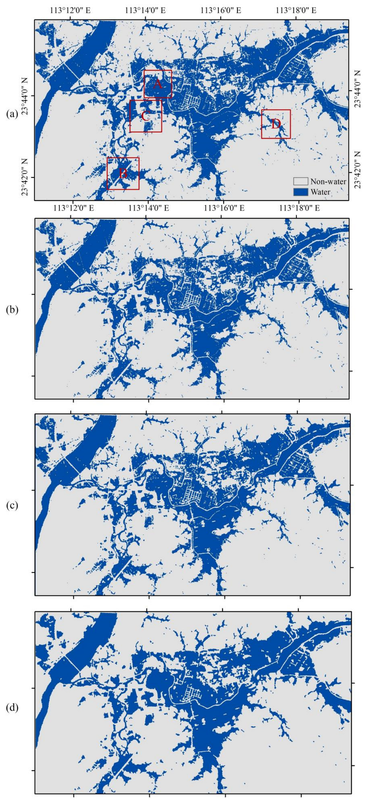
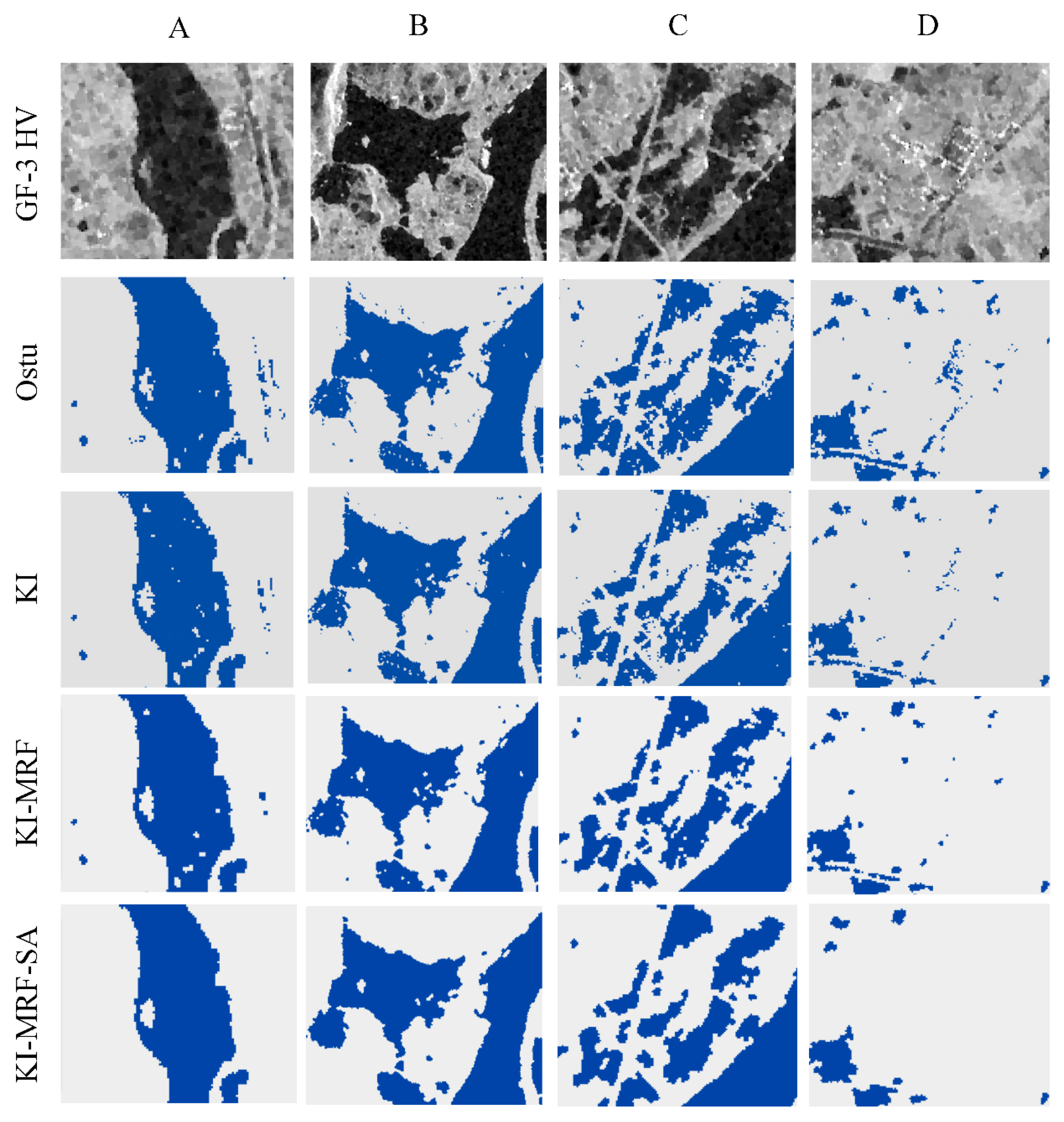
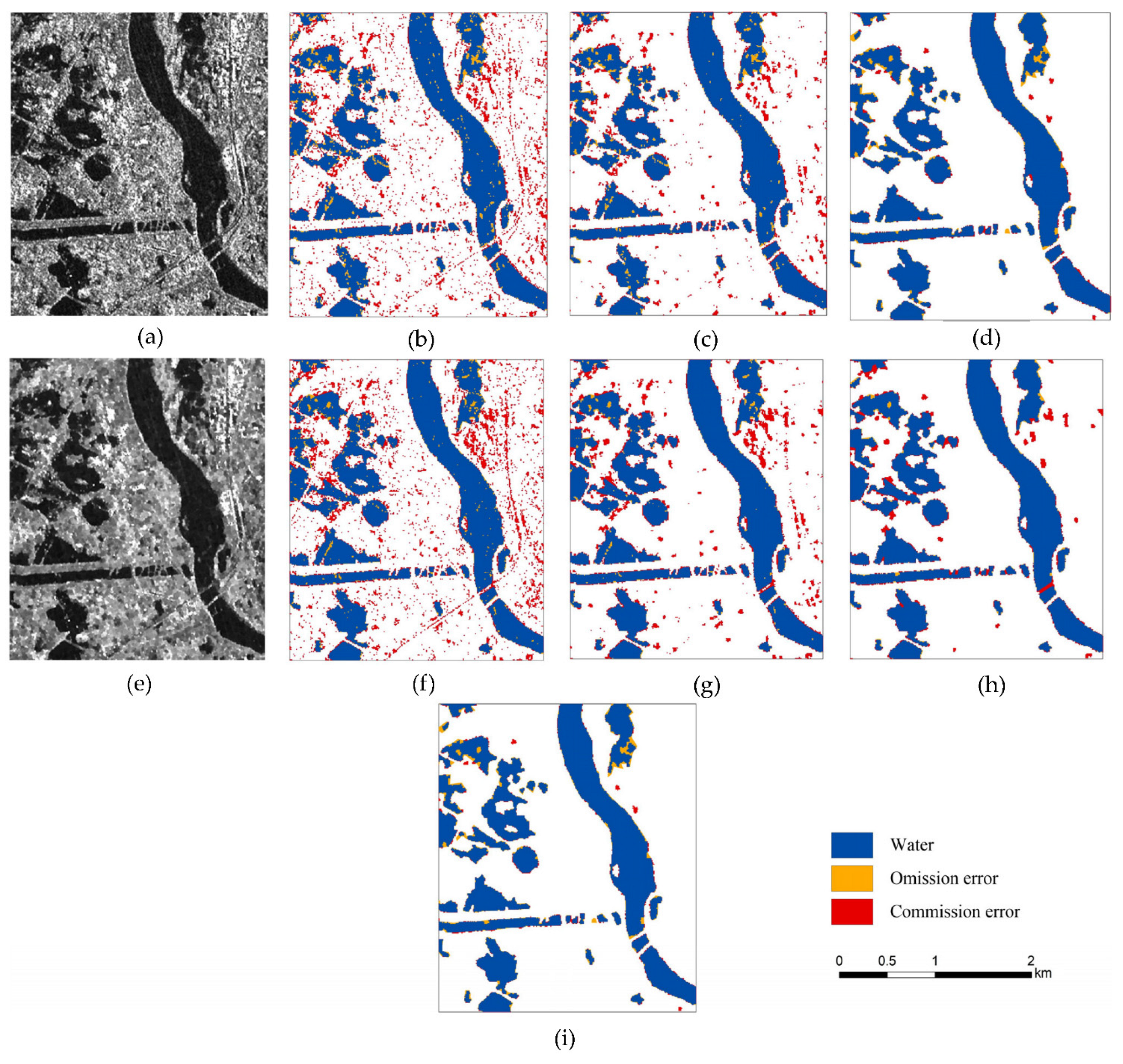
4.1. Water Extraction

Four water extraction schemes were adopted as a means to verify the effectiveness of the method proposed in this research: Otsu, KI, KI-MRF, and KI-MRF-SA. Otsu and KI verify the effectiveness of cases that only utilize Otsu’s and KI’s thresholding segmentation for water extraction, respectively. KI-MRF verifies the effectiveness of cases that utilize MRF for water extraction based on KI’s thresholding segmentation method. KI-MRF-SA is the final scheme proposed in this paper, which indicates the effectiveness of the combination of the MRF and SA methods for water extraction based on KI’s thresholding segmentation method. Each scheme has made improvements on some key steps compared to the previous one, and the last scheme incorporates all of the improvements.
To ensure accuracy and comparability, the four schemes utilized the same parameters in the same step, including energy weight parameters h ,     β ,     η , the maximum number of iterations kmax, etc. For the quantitative evaluation, a total of one thousand sampling points were randomly generated within the two experimental areas. These points were labelled through visual interpretation, which enabled a comparison of the accuracy of the four schemes.
The quantitative evaluation results of the four schemes are listed in Table 2. The OAs of these methods are above 88%, because the majority of the image points are non-water areas and they are most accurately delineated, thus inflating the OA. In the extraction process of the flood inundation, more attention should be paid to the accuracy indicators related to water. The OAs of Otsu’s and KI’s threshold segmentation methods are approximately 88.60%, and 90.50%, respectively, which demonstrates the robustness of these two classical segmentation methods. However, in the case of Otsu’s method, there is a higher commission error rate, with the lowest UA of 84.90%. The UA of KI’s threshold segmentation is 86.51%, which is relatively superior to Otsu, indicating that the water extraction results obtained through KI’s threshold segmentation are more accurate. Both KI’s and Otsu’s methods do not take the spatial neighborhood information into consideration, which leads to a large number of noise errors in the results and a PA of only 88.35% and 88.31%, respectively.
As compared with simple thresholding segmentation, the method proposed in this study is capable of producing more accurate results for various indicators. The KI-MRF method can reduce a number of small noise errors through MRF, thus directly improving the UA and PA of the water extraction results by approximately 1% and 2.5%, respectively. On this basis, KI-MRF-SA employs the SA algorithm as a means to further improve the results, making the effect of noise reduction reach the global optimum. In the case of KI-MRF-SA, there was an increase in the UA and PA of the water extraction results by approximately 2.5% and 1.8%, reaching 89.82 and 92.65%, respectively. As a result of improving the method proposed in this research, there was an increase in the OA and Kappa coefficients. Compared with the KI method, KI-MRF-SA showed an increase of about 2.4% in total in OA, and the Kappa coefficient increased by 0.03, indicating that KI-MRF-SA is capable of effectively improving the accuracy of the water detection method.
Figure 6, Figure 7, Figure 8 and Figure 9 show the water extraction results, in addition to enlarged images of the four schemes. In terms of the overall extraction effect, they are consistent with the previous quantitative analysis results. There is a large amount of noise in the results of Otsu’s and KI’s methods. The KI-MRF method is capable of effectively reducing part of the noise, and KI-MRF-SA can further reduce the noise level and achieve the best extraction effect.
According to the enlarged image, Otsu’s and KI’s methods misclassify some isolated pixels of water as non-water; those must be classified as water pixels with higher backscatter intensities due to the SAR speckle noise occurring in a homogenous surface, as shown at spots A, B, and C in Figure 7 and spots A, B, and C in Figure 9. Additionally, some non-water pixels with lower backscattering intensities are misclassified as water, as shown at spot D in Figure 7 and spot D in Figure 9. The main reason for this is that a smooth land surface may also lead to a lower backscattering intensity. Therefore, omission and commission errors are hard to avoid with only threshold segmentation.
Regarding threshold segmentation, the KI-MRF method employs MRF to further optimize the segmentation result. Some isolated and small noises can be easily reduced, but some dense and large noises are still difficult to eliminate, as shown at spot A in Figure 7 and spot A in Figure 9. The KI-MRF-SA method is capable of “melting” this part of the noise with the global optimization capability of SA and can obtain the best water extraction results. The contrast experiment of water extraction proves that the combination of MRF and SA can effectively take advantage of the spatial neighborhood information in order to eliminate omission and commission errors, thereby improving the accuracy of water extraction results.

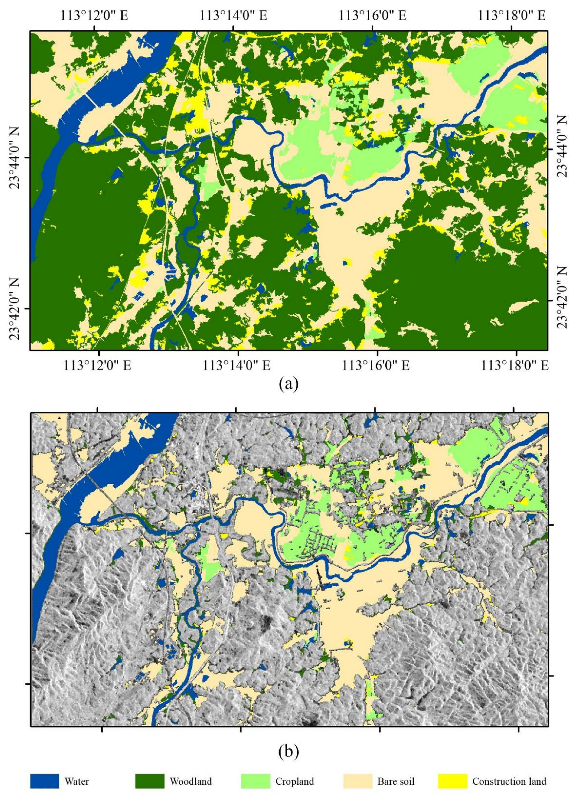
4.2. Classification of Inundated Areas

OSA-CNN was utilized for the classification of GF-2 images in order to determine the types of land cover before the occurrence of floods, as shown in Figure 10a and Figure 11a. The flood inundation map was obtained by employing the superimposed flood inundation extent and land cover types, as shown in Figure 10b and Figure 11b.
According to the statistics of the flood-affected areas in the experimental areas, the total flood-affected areas of Boluokeng and Pajiang measured 8.99 km2 and 24.83 km2, respectively, among which the cropland, woodland, bare soil, and construction lands of Boluokeng measured 6.62 km2, 1.69 km2, 0.32 km2, and 0.36 km2, respectively, and those of Pajiang measured 4.89 km2, 1.84 km2, 17.44 km2, and 0.66 km2, respectively.
On the basis of the statistical results, the land type of the flood-affected area in Boluokeng was mainly cropland, accounting for 73.6% of the flooded area, followed by woodland, accounting for 18.8%. As shown in Figure 10, the flood-affected cropland and woodland were mainly distributed in the plains on both sides of the river, and the surrounding higher-lying woodland was less affected. The construction land in the northeast was also less affected due to the construction of dams along the river. Pajiang is located in the downstream plain with open and low-lying terrain, and since the accumulated water cannot be easily discharged, it resulted in a large flooded area. Flood-affected areas were predominantly composed of bare soil and cropland, accounting for 70.2%, and 19.7% of the total. As shown in Figure 11, the flood spread from the south side of the river to the surrounding mountains. Although there is a dam built on the north side of the river, the long-term heavy rain caused the dam to overflow, causing a large area of cropland to be flooded on the north side.
Since the extraction accuracy of the flood inundation area has been verified previously, only the classification accuracy verification is required to be carried out within those areas. For this purpose, a total of one thousand sample points were randomly selected from the flooded areas of the two experimental areas, and their land types were manually labelled with reference to the GF-2 image. Subsequently, a confusion matrix was employed as a means for accuracy validation, as shown in Table 3. In this case, the OA of the classification result is 92.7%, and the classification accuracy of water, cropland, and bare soil is higher, with a PA and UA exceeding 90%, while the PA and UA of woodland and construction land are relatively lower, at approximately 82% and 88%, respectively. Due to the relatively small proportion of woodland and construction land within the flooded area, and the fact that they are dispersed, the CNN results are easily disturbed by ground objects.
In our previous studies [47], the OSA-CNN method was capable of achieving approximately a 90% OA and a 0.87 Kappa in the case of the GF-2 image classification. Compared with that, in this study, the classification process was able to achieve superior results in the cases of OA and Kappa, reaching 92.7% and 0.9, respectively. This is due to the fact that this experiment mainly focused on flood-affected areas, where the terrain is flat and there is no interference from mountain shadows. Moreover, in this experiment, the main types of land used were cropland and bare soil, both of which have relatively simple characteristics and homogeneous distributions, which facilitate a more accurate classification process.

5. Discussion

In this research, two automatic thresholding methods, Otsu and KI, are employed for the segmentation of SAR images of GF-3. In this procedure, the automatic thresholds are compared with the visual interpretation threshold, and the influence of different polarizations on the thresholding segmentation results is discussed. As shown in Table 4, the thresholds of Otsu’s method are generally higher, with a difference of approximately 1–2 dB from the visual interpretation threshold, which may lead to an increase in the commission error rate. However, the difference between KI’s threshold and the visual interpretation threshold is relatively small, with less than 0.5 dB in different polarizations, indicating that the result of KI’s thresholding method is closer to the real distribution of water, which is consistent with the results of the quantitative evaluation. In addition, the thresholds of the two methods in the HV polarization are closer to the results of the visual interpretation thresholds than the HH polarization, indicating that water detection in the HV polarization is more stable.
Speckle noise is a characteristic of SAR images regardless of imaging modes, resulting in abrupt variations of pixel intensity in homogeneous regions and a high number of omission and commission errors, as depicted in Figure 12b,f. Typically, speckle noise can be reduced by applying low-pass filtering to images, such as the refined Lee speckle filter adopted in the preprocessing section of this study, as depicted in Figure 12c,g. In some complex regions, however, speckle noise cannot be entirely eliminated by filtering, and excessive filtering may impair image resolution. In this study, KI-MRF-SA was adopted for morphological optimization. The advantage is that only local noise was processed so as to avoid image detail loss caused by global filtering, as illustrated in Figure 12d,h.
The KI-MRF-SA method was applied to each polarization of the image, and an intersection operation was used to aggregate the water extents from two polarizations (HH and HV). The water maps derived from HH and HV are distinct because scatters within the same scene exhibit varying scattering strengths in different polarization modes. In general, strong HH signals are associated with rough surface scattering, whereas HV signals are typically more susceptible to volume scattering. Applying the intersection of the two polarizations can reduce commission error by masking rough surfaces or volume scatterers with high backscattering, though it may slightly increase the omission error, as depicted in Figure 12i.
In the KI-MRF-SA method, the temperature control parameter s directly affects the convergence rate in energy decline; thus, a further examination of the impact of different s values is warranted. In this regard, taking the HV polarization of Boluokeng as an example, s was set as 0, 0.005, 0.01, and 0.02, respectively, and the other parameters remained constant. Then, we calculated the global energy change, as shown in Table 5. s = 0 means that SA is not involved in the iterative operation, which is the KI-MRF method proposed in this research. KI-MRF is characterized by a fast convergence speed, and the global energy of the image tends to be stable after applying the second iteration. However, due to the incomplete noise elimination, the energy of convergence is relatively high, approximately −7233. As s increases, the convergence speed of the energy slows down. When s is set as 0.005, 0.01, and 0.02, the corresponding convergence iterations are 4, 7, and 10, respectively, and the corresponding energies are −7247, −7251, and −7251. This demonstrates that the energy convergence reaches the minimum when s is 0.01, and as s increases further, the convergence time is prolonged rather than the energy being reduced.
We proposed a novel water extraction method for SAR imagery based on MRF and SA. Compared with the traditional threshold method, this method can reduce the classification error caused by speckle noise more efficiently, allowing for greater accuracy. The method is unsupervised, efficient, and suitable for near real-time flood detection. However, in densely populated metropolitan regions, tall buildings can hinder the applicability of SAR images. Owing to the side-looking nature of the sensor, building shadows with low brightness intensities would be classified as water. On the other hand, the corners formed by buildings and the ground can produce a double bounce effect, resulting in bright pixels in the image. When these corners are flooded, the image pixels appear to be brighter, which causes threshold methods to misclassify them. Based on the discussion above, flood extraction in high development density areas needs to further improve for flood mapping strategies. In future studies, additional data sources, such as UAV images, will be considered to improve the classification accuracy, or time series SAR images will be used to overcome the problem of smooth surfaces with low backscattering. In this study, only a single-temporal SAR image was utilized to identify the flood inundation area; however, the proposed method can be simply applied to multi-temporal images to detect inundation changes.

6. Conclusions

The earth observation technology of remote sensing has always been the key means of flood monitoring, and the combination of optical remote images and SAR images for the extraction of flood inundation information is a promising application mode. Optical images provide clear imaging and rich features, while SAR imaging provides 24 h and all-weather characteristics, making it possible to obtain information about inundation extent after floods as well as land cover types prior to floods, thus improving the classification of flood inundation areas. In this study, the combination of KI’s threshold segmentation, MRF, and SA algorithms is applied to the water extraction process in SAR images, and the technical framework of “extraction and then refinement” is adopted in order to form a more flexible KI-MRF-SA method. The experimental results of Boluokeng and Pajiang’s Gaofen-3 satellite images demonstrate that, in comparison with the traditional threshold method, KI-MRF-SA offers advantages in terms of water extraction, retaining the quality of image details while reducing the impact of noise. Combined with the classification method of OSA-CNN proposed in our previous research, the classification of flood-affected areas can be further realized on the basis of high-precision identification of the flood inundation extent.
Although threshold segmentation still needs to be improved, since only a small scale of water extraction is investigated in this study, a single threshold may not be sufficient to distinguish between larger scales of water extraction. Therefore, our future work will focus on multi-threshold segmentation and local threshold segmentation in order to develop more robust threshold segmentation methods.
The findings of this study demonstrate that the comprehensive utilization of SAR and optical images can accurately identify the land cover type and extent of the flood inundation area. The direct value of this study is to enable emergency managers to fulfill their need for collecting near real-time flood inundation maps, so as to offer auxiliary decision-making for disaster relief measures in different flooded areas, and provide data support for disaster assessment. Hence, the method proposed in this paper can represent a valuable tool to pursue this objective.
Moreover, the added value of this study is that it paves the way for the development of novel applications in flood disaster management. For instance, sequential flood coverage monitoring data can be utilized to regularly update/correct flood computation models through data assimilation procedures, as well as to estimate pertinent variables such as river discharge and channel depth. Other studies have demonstrated that flood inundation maps obtained from satellite earth observation are of great value in lowering the prediction uncertainty of numerical models and generating essential hydrological variables [62,63,64]. However, given that this study method has not been implemented in other instances, further verification of its efficacy is required and is planned for the near future.

Author Contributions

Methodology, J.W.; Validation, J.W.; Writing—original draft, J.W.; Supervision, B.H. and F.W.; Funding acquisition, B.H. All authors have read and agreed to the published version of the manuscript.

Funding

This research was funded by the China Postdoctoral Science Foundation (No. 2022M710837), the Key-Area Research and Development Program of Guangdong Province (No. 2020B0101130018), and the GuangDong Basic and Applied Basic Research Foundation (No. 202201011275).

Data Availability Statement

The data presented in this study are available on request from the corresponding author. The data are not publicly available due to privacy.

Acknowledgments

The authors gratefully acknowledge the contribution of many research fellows in the Guangdong Provincial Science and Technology Collaborative Innovation Center for Water Safety and the Guangdong Key Scientific Research Base of Hydraulics.

Conflicts of Interest

The authors declare no conflict of interest.

References

  1. Liang, Y.; Liu, D. A local thresholding approach to flood water delineation using Sentinel-1 SAR imagery. ISPRS J. Photogramm. Remote Sens. 2020, 159, 53–62. [Google Scholar] [CrossRef]
  2. Adhikari, P.; Hong, Y.; Douglas, K.R.; Kirschbaum, D.B.; Gourley, J.; Adler, R.; Robert Brakenridge, G. A digitized global flood inventory (1998–2008): Compilation and preliminary results. Nat. Hazards. 2010, 55, 405–422. [Google Scholar] [CrossRef]
  3. Hallegatte, S.; Green, C.; Nicholls, R.J.; Corfee-Morlot, J. Future flood losses in major coastal cities. Nat. Clim. Chang. 2013, 3, 802–806. [Google Scholar] [CrossRef]
  4. Schumann, G.J.P.; Bates, P.D.; Di Baldassarre, G.; Mason, D.C. Chapter 6 The Use of Radar Imagery in Riverine Flood Inundation Studie. In Fluvial Remote Sensing for Science and Management; John Wiley & Sons: Hoboken, NJ, USA, 2012; pp. 115–140. [Google Scholar]
  5. Pall, P.; Aina, T.; Stone, D.A.; Stott, P.A.; Nozawa, T.; Hilberts, A.G.J.; Lohmann, D.; Allen, M.R. Anthropogenic greenhouse gas contribution to flood risk in England and Wales in autumn 2000. Nature 2011, 470, 382–385. [Google Scholar] [CrossRef]
  6. Martinez, J.M.; Le Toan, T. Mapping of flood dynamics and spatial distribution of vegetation in the Amazon floodplain using multitemporal SAR data. Remote Sens. Environ. 2007, 108, 209–223. [Google Scholar] [CrossRef]
  7. Tralli, D.M.; Blom, R.G.; Zlotnicki, V.; Donnellan, A.; Evans, D.L. Satellite remote sensing of earthquake, volcano, flood, landslide and coastal inundation hazards. ISPRS J. Photogramm. Remote Sens. 2005, 59, 185–198. [Google Scholar] [CrossRef]
  8. Kuenzer, C.; Guo, H.; Schlegel, I.; Tuan, V.; Li, X.; Dech, S. Varying scale and capability of Envissat ASAR-WSM, TerraSAR-X Scansar and TerraSAR-X Stripmap data to assess urban flood situations: A case study of the mekong delta in can tho province. Remote Sens. 2013, 5, 5122–5142. [Google Scholar] [CrossRef] [Green Version]
  9. Mason, D.C.; Giustarini, L.; Garcia-Pintado, J.; Cloke, H.L. Detection of flooded urban areas in high resolution Synthetic Aperture Radar images using double scattering. Int. J. Appl. Earth Obs. Geoinf. 2014, 28, 150–159. [Google Scholar] [CrossRef] [Green Version]
  10. O’Grady, D.; Leblanc, M.; Bass, A. The use of radar satellite data from multiple incidence angles improves surface water mapping. Remote Sens. Environ. 2014, 140, 652–664. [Google Scholar] [CrossRef]
  11. Schumann, G.J.P.; Neal, J.C.; Mason, D.C.; Bates, P.D. The accuracy of sequential aerial photography and SAR data for observing urban flood dynamics, a case study of the UK summer 2007 floods. Remote Sens. Environ. 2011, 115, 2536–2546. [Google Scholar] [CrossRef]
  12. Ulaby, F.; Dobson, M.C. Handbook of Radar Scattering Statistics for Terrain; Artech House: Norwood, MA, USA, 1989. [Google Scholar]
  13. Chaouch, N.; Temimi, M.; Hagen, S.; Weishampel, J.; Medeiros, S.; Khanbilvardi, R. A synergetic use of satellite imagery from SAR and optical sensors to improve coastal flood mapping in the Gulf of Mexico. Hydrol. Process. 2011, 26, 1617–1628. [Google Scholar] [CrossRef] [Green Version]
  14. Chung, H.W.; Liu, C.C.; Cheng, I.F.; Lee, Y.R.; Shieh, M.C. Rapid response to a typhoon-induced flood with an SAR-derived map of inundated areas: Case study and validation. Remote Sens. 2015, 7, 11954–11973. [Google Scholar] [CrossRef] [Green Version]
  15. Gstaiger, V.; Huth, J.; Gebhardt, S.; Wehrmann, T.; Kuenzer, C. Multi-sensoral and automated derivation of inundated areas using TerraSAR-X and ENVISAT ASAR data. Int. J. Remote Sens. 2012, 33, 7291–7304. [Google Scholar] [CrossRef]
  16. Boni, G.; Ferraris, L.; Pulvirenti, L.; Squicciarino, G.; Pierdicca, N.; Candela, L.; Pisani, A.R.; Zoffoli, S.; Onori, R.; Proietti, C.; et al. A prototype system for flood monitoring based on flood forecast combined with COSMO-SkyMed and Sentinel-1 Data. IEEE J. Sel. Top. Appl. Earth Obs. Remote Sens. 2016, 9, 2794–2805. [Google Scholar] [CrossRef]
  17. Chini, M.; Hostache, R.; Giustarini, L.; Matgen, P. A hierarchical split-based approach for parametric thresholding of SAR images: Flood inundation as a test case. Geosci. Remote Sens. IEEE Trans. 2017, 55, 6975–6988. [Google Scholar] [CrossRef]
  18. Greifeneder, F.; Wagner, W.; Sabel, D.; Naeimi, V. Suitability of SAR imagery for automatic flood mapping in the Lower Mekong Basin. Int. J. Remote Sens. 2014, 35, 2857–2874. [Google Scholar] [CrossRef]
  19. Martinis, S.; Kersten, J.; Twele, A. A fully automated TerraSAR-X based flood service. ISPRS J. Photogramm. Remote Sens. 2015, 104, 203–212. [Google Scholar] [CrossRef]
  20. Martinis, S.; Twele, A.; Strobl, C.; Kersten, J.; Stein, E. A multi-scale flood monitoring system based on fully automatic MODIS and TerraSAR-X processing chains. Remote Sens. 2013, 5, 5598–5619. [Google Scholar] [CrossRef] [Green Version]
  21. Martinis, S.; Twele, A.; Voigt, S. Towards operational near real-time flood detection using a split-based automatic thresholding procedure on high resolution TerraSAR-X data. Nat. Hazards Earth Syst. Sci. 2009, 9, 303–314. [Google Scholar] [CrossRef]
  22. Twele, A.; Cao, W.; Plank, S.; Martinis, S. Sentinel-1-based flood mapping: A fully automated processing chain. Int. J. Remote Sens. 2016, 37, 2990–3004. [Google Scholar] [CrossRef]
  23. Iervolino, P.; Guida, R.; Iodice, A.; Riccio, D. Flooding water depth estimation with high-resolution SAR. IEEE Trans. Geosci. Remote Sens. 2015, 53, 2295–2307. [Google Scholar] [CrossRef] [Green Version]
  24. Chini, M.; Pulvirenti, L.; Pierdicca, N. Analysis and interpretation of the COSMO-SkyMed observations of the 2011 Japan Tsunami. IEEE Geosci. Remote Sens. Lett. 2012, 9, 467–471. [Google Scholar] [CrossRef]
  25. Pulvirenti, L.; Chini, M.; Pierdicca, N.; Boni, G. Use of SAR data for detecting floodwater in urban and suburban areas: The role of the interferometric coherence. IEEE Trans. Geosci. Remote Sens. 2016, 54, 1532–1544. [Google Scholar] [CrossRef]
  26. Pulvirenti, L.; Pierdicca, N.; Chini, M.; Guerriero, L. Monitoring flood evolution in vegetated areas using COSMO-SkyMed data: The Tuscany 2009 case study. IEEE J. Sel. Topics Appl. Earth Obs. Remote Sens. 2013, 6, 1807–1816. [Google Scholar] [CrossRef]
  27. Tsyganskaya, V.; Martinis, S.; Marzahn, P.; Ludwig, R. Detection of temporary flooded vegetation using Sentinel-1 time series data. Remote Sens. 2018, 10, 1286. [Google Scholar] [CrossRef] [Green Version]
  28. Tsyganskaya, V.; Martinis, S.; Marzahn, P.; Ludwig, R. SAR-based detection of flooded vegetation—A review of characteristics and approaches. Int. J. Remote Sens. 2018, 39, 2255–2293. [Google Scholar] [CrossRef]
  29. Pierdicca, N.; Pulvirenti, L.; Boni, G.; Squicciarino, G.; Chini, M. Mapping flooded vegetation using COSMO-SkyMed: Comparison with polarimetric and optical data over rice fields. IEEE J. Sel. Topics Appl. Earth Obs. Remote Sens. 2017, 10, 2650–2662. [Google Scholar] [CrossRef]
  30. Giustarini, L.; Hostache, R.; Matgen, P.; Schumann, G.J.P.; Bates, P.D.; Mason, D.C. A change detection approach to flood mapping in urban areas using TerraSAR-X. IEEE Trans. Geosci. Remote Sens. 2013, 51, 2417–2430. [Google Scholar] [CrossRef] [Green Version]
  31. Hostache, R.; Matgen, P.; Wagner, W. Change detection approaches for flood extent mapping: How to select the most adequate reference image from online archives? Int. J. Appl. Earth Obs. Geoinf. 2012, 19, 205–213. [Google Scholar] [CrossRef]
  32. Pierdicca, N.; Chini, M.; Pulvirenti, L.; Macina, F. Integrating physical and topographic information into a fuzzy scheme to map flooded area by SAR. Sensors 2008, 8, 4151–4164. [Google Scholar] [CrossRef] [Green Version]
  33. Pierdicca, N.; Pulvirenti, L.; Chini, M. Flood mapping in vegetated and urban areas and other challenges: Models and methods. In Flood Monitoring through Remote Sensing; Refice, A., D’Addabbo, A., Capolongo, D., Eds.; Springer: Cham, Switzerland, 2018; pp. 135–179. [Google Scholar]
  34. Girshick, R.; Donahue, J.; Darrell, T.; Malik, J. Region-based convolutional networks for accurate object detection and segmentation. IEEE Trans. Pattern Anal. Mach. Intell. 2016, 38, 142–158. [Google Scholar] [CrossRef]
  35. Kussul, N.; Lavreniuk, M.; Skakun, S.; Shelestov, A. Deep learning classification of land cover and crop types using remote sensing data. IEEE Geosci. Remote Sens. Lett. 2017, 14, 778–782. [Google Scholar] [CrossRef]
  36. Zhu, X.; Tuia, D.; Mou, L.; Xia, G.; Zhang, L.; Xu, F. Deep learning in remote sensing: A comprehensive review and list of resources. IEEE Geosci. Remote Sens. 2017, 5, 8–36. [Google Scholar] [CrossRef] [Green Version]
  37. Cheng, G.; Han, J.; Lu, X. Remote sensing image scene classification: Benchmark and state-of-the-art. Proc. IEEE. 2017, 105, 1865–1883. [Google Scholar] [CrossRef] [Green Version]
  38. Cheng, G.; Yang, C.; Yao, X.; Guo, L.; Han, J. When deep learning meets metric learning: Remote sensing image scene classification via learning discriminative CNNs. IEEE Trans. Geosci. Remote Sens. 2018, 56, 2811–2821. [Google Scholar] [CrossRef]
  39. Zhou, Q.; Zhou, Y.; Zhang, L.; Li, D. Adaptive deep sparse semantic modeling framework for high spatial resolution image scene classification. IEEE Trans. Geosci. Remote Sens. 2018, 56, 6180–6195. [Google Scholar] [CrossRef]
  40. Li, E.; Xia, J.; Du, P.; Ling, C.; Samat, A. Integrating multi-layer features of convolutional neural networks for remote sensing scene classification. IEEE Trans. Geosci. Remote Sens. 2017, 55, 5653–5665. [Google Scholar] [CrossRef]
  41. Du, P.; Li, E.; Xia, J.; Samat, A.; Bai, X. Feature and model level fusion of pretrained CNN for remote sensing scene classification. IEEE J. Sel. Topics Appl. Earth Obs. Remote Sens. 2019, 12, 2600–2611. [Google Scholar] [CrossRef]
  42. Hu, F.; Xia, G.; Yang, W.; Zhang, L. Mining deep semantic representations for scene classification of high-resolution remote sensing imagery. IEEE Trans. Big Data. 2019, 6, 522–536. [Google Scholar] [CrossRef]
  43. Zhao, W.; Du, S.; Emery, W.J. Object-based convolutional neural network for high-resolution imagery classification. IEEE J. Sel. Topics Appl. Earth Obs. Remote Sens. 2017, 10, 3386–3396. [Google Scholar] [CrossRef]
  44. Xu, Y.; Du, B.; Zhang, F.; Zhang, L. Hyperspectral image classification via a random patches network. ISPRS J. Photogramm. Remote Sens. 2018, 142, 344–357. [Google Scholar] [CrossRef]
  45. Huang, B.; Zhao, B.; Song, Y. Urban land-use mapping using a deep convolutional neural network with high spatial resolution multispectral remote sensing imagery. Remote Sens. Environ. 2018, 214, 73–86. [Google Scholar] [CrossRef]
  46. Zhou, S.; Xue, Z.; Du, P. Semisupervised stacked autoencoder with cotraining for hyperspectral image classification. IEEE Trans. Geosci. Remote Sens. 2019, 57, 3813–3826. [Google Scholar] [CrossRef]
  47. Wang, J.; Zheng, Y.; Shen, Q.; Huang, J. Object-Scale Adaptive Convolutional Neural Networks for High-Spatial Resolution Remote Sensing Image Classification. IEEE J. Sel. Topics Appl. Earth Obs. Remote Sens. 2020, 14, 283–299. [Google Scholar] [CrossRef]
  48. Otsu, N. A threshold selection method from gray-level histograms. IEEE Trans. Syst. Man Cybern. 1979, 9, 62–66. [Google Scholar] [CrossRef] [Green Version]
  49. Kittler, J.; Illingworth, J. Minimum error thresholding. Pattern Recogn. 1986, 19, 41–47. [Google Scholar] [CrossRef]
  50. Bazi, Y.; Bruzzone, L.; Melgani, F. An unsupervised approach based on the generalized Gaussian model to automatic change detection in multitemporal SAR images. IEEE Trans. Geosci. Remote Sens. 2005, 43, 874–887. [Google Scholar] [CrossRef] [Green Version]
  51. Melgani, F.; Moser, G.; Serpico, S.B. Unsupervised change-detection methods for remote-sensing images. Opt. Eng. 2002, 41, 3288–3297. [Google Scholar]
  52. Bovolo, F.; Bruzzone, L. A split-based approach to unsupervised change detection in large-size SAR images. IEEE Trans. Geosci. Remote Sens. 2007, 45, 1658–1670. [Google Scholar] [CrossRef]
  53. Moser, G.; Serpico, S.B. Generalized Minimum-Error Thresholding for Unsupervised Change Detection From SAR Amplitude Imagery. IEEE Trans. Geosci. Remote Sens. 2006, 44, 2972–2982. [Google Scholar] [CrossRef]
  54. Besag, J. On the Statistical-Analysis of Dirty Pictures. J. R. Stat. Society. Ser. B Methodol. 1986, 48, 259–302. [Google Scholar] [CrossRef] [Green Version]
  55. Kirkpatrick, S.; Gelatt, C.D.; Vecchi, A. Optimization by Simulated Annealing. Science 1983, 220, 671–680. [Google Scholar] [CrossRef] [PubMed]
  56. Metropolis, N.; Rosenbluth, A.W.; Rosenbluth, M.N.; Taller, A.H.; Teller, E. Equation of State by Fast Computing Machines. J. Chem. Phys. 1953, 21, 1087–1092. [Google Scholar] [CrossRef] [Green Version]
  57. Wang, M.; Wang, J. A Region-Line Primitive Association Framework for Object-Based Remote Sensing Image Analysis. Photogramm. Eng. Remote Sens. 2016, 82, 149–159. [Google Scholar] [CrossRef]
  58. Wang, M.; Li, R. Segmentation of High Spatial Resolution Remote Sensing Imagery Based on Hard-Boundary Constraint and Two-Stage Merging. IEEE Trans. Geosci. Remote Sens. 2014, 52, 5712–5725. [Google Scholar] [CrossRef]
  59. Wang, M.; Xing, J.; Wang, J.; Lv, G. Technical design and system implementation of region-line primitive association framework. ISPRS J. Photogramm. Remote Sens. 2017, 130, 202–216. [Google Scholar] [CrossRef]
  60. Wang, M.; Cui, Q.; Wang, J.; Ming, D.; Lv, G. Raft cultivation area extraction from high resolution remote sensing imagery by fusing multi-scale region-line primitive association features. ISPRS J. Photogramm. Remote Sens. 2017, 123, 104–113. [Google Scholar] [CrossRef]
  61. Wang, M.; Cui, Q.; Sun, Y.; Wang, Q. Photovoltaic panel extraction from very high-resolution aerial imagery using region–line primitive association analysis and template matching. ISPRS J. Photogramm. Remote Sens. 2018, 141, 100–111. [Google Scholar] [CrossRef]
  62. Oubanas, H.; Gejadze, I.; Malaterre, P.O.; Mercier, F. River discharge estimation from synthetic SWOT-type observations using variational data assimilitation and the full Saint-Venant hydrualic model. J. Hydrol. 2018, 559, 638–647. [Google Scholar] [CrossRef]
  63. Hostache, R.; Chini, M.; Giustarini, L.; Neal, J.; Kavetski, D.; Wood, M.; Corato, G.; Pelich, R.M.; Matgen, P. Near-real-time assimilation of SAR-derived flood maps for improving flood forecasts. Water Resour. Res. 2018, 54, 5516–5535. [Google Scholar] [CrossRef]
  64. Bates, P.D. Remote sensing and flood inundation modelling. Hydrol. Process. 2002, 18, 2593–2597. [Google Scholar] [CrossRef]
Figure 1. GF-3 images of Boluokeng and Pajiang.
Water 15 01288 g001
Figure 2. GF-2 images of the two experimental areas: (a) Boluokeng; (b) Pajiang.
Water 15 01288 g002
Figure 3. Main technical process of proposed method.
Water 15 01288 g003
Figure 4. (a,b) are the water/non-water histograms of HV and HH polarization of the Boluokeng area, respectively. (c,d) are the water/non-water histograms of HV and HH polarization of the Pajiang area, respectively.
Water 15 01288 g004
Figure 5. (a) GF-2 image. (b) The segmentation results. (c) The axis extraction from an object primitive. (d) The image patches sampled along the axes. (e) The classification results of image patches. (f) The classification result of an object primitive.
Water 15 01288 g005
Figure 6. Water delineated by using (a) Otsu’s method, (b) KI’s method, (c) the KI-MRF algorithm, and (d) the KI-MRF-SA algorithm in Boluokeng. The red boxes mark some remarkably changed spots (A, B, C and D) and method enhancements.
Water 15 01288 g006
Figure 7. Detail displays of water extraction in Boluokeng. The subfigures (AD) are some remarkably changed spots in Boluokeng.
Water 15 01288 g007
Figure 8. Water delineated by using (a) Otsu’s method, (b) KI’s method, (c) the KI-MRF algorithm, and (d) the KI-MRF-SA algorithm in Pajiang. The red boxes mark some remarkably changed spots (A, B, C and D) and method enhancements.
Water 15 01288 g008
Figure 9. Detail displays of water extraction in Pajiang. The subfigures (AD) are some remarkably changed spots in Pajiang.
Water 15 01288 g009
Figure 10. (a) The OSA-CNN classification result in Boluokeng. (b) The flood inundation map in Boluokeng.
Water 15 01288 g010
Figure 11. (a) The OSA-CNN classification result in Pajiang. (b) The flood inundation map in Pajiang.
Water 15 01288 g011
Figure 12. (a) HH polarimetric SAR image. (bd) are the water maps derived from (a), which are processed by KI, refined Lee filter + KI, and refined Lee + KI-MRF-SA respectively. (e) HV polarimetric SAR image. (fh) are the water maps derived from (e), which are processed by KI, refined Lee filter + KI, and refined Lee + KI-MRF-SA respectively. (i) The intersection of (d,h).
Water 15 01288 g012
Table 1. Summary of remote sensing data used in this study.
ImageLocationRemote SensorAcquisition DateSize (Pixel)Resolution (m)
Boluokeng113°23′51″ EGF-3 (FSII)24 June 20221045 × 141110 × 10
24°7′23″ NGF-211 November 20211972 × 27684 × 4
Pajiang113°14′56″ EGF-3 (FSII)24 June 20222099 × 131910 × 10
23°43′31″ NGF-211 November 20213160 × 19534 × 4
Table 2. Accuracy assessment of water and non-water delineation using different methods.
MethodUA (%)PA (%)OA (%)Kappa
WaterNon-WaterWaterNon-Water
Otsu84.9092.8788.3590.6188.600.77
KI86.5192.6288.3191.4290.500.80
KI-MRF87.4194.2090.8491.9191.500.82
KI-MRF-SA89.8295.3892.6593.5393.100.85
Table 3. Accuracy assessment of the land cover classification of the flooded area.
User/Reference ClassWaterCroplandBare SoilWoodlandConstruction LandSum
Water18510620203
Cropland10257952283
Bare soil0838210391
Woodland32675389
Construction land01232834
Sum1982784058633
PA (%)93.492.494.387.284.8
UA (%)91.190.897.784.382.4
OA (%)92.7
Kappa0.90
Table 4. The comparison of thresholds using different threshold segmentation methods.
ImageVisual Interpretation (dB)Otsu (dB)KI (dB)
Boluokeng HV−29−28.02−29.20
Boluokeng HH−23−21.12−22.80
Pajiang HV−32−30.56−31.90
Pajiang HH−24−22.31−23.64
Table 5. Global energy change in the HV polarization of Boluokeng during the iterative operation.
kEnergy
s = 0s = 0.005s = 0.01s = 0.02
0−7198−7198−7198−7198
1−7231−6838−4339−1522
2−7233−7216−6569−4236
3−7233−7240−7167−5933
4−7233−7246−7229−6876
5−7233−7246−7248−7146
6−7233−7246−7250−7211
7−7233−7247−7251−7231
8−7233−7247−7251−7243
9−7233−7247−7251−7250
10−7233−7247−7251−7251
Disclaimer/Publisher’s Note: The statements, opinions and data contained in all publications are solely those of the individual author(s) and contributor(s) and not of MDPI and/or the editor(s). MDPI and/or the editor(s) disclaim responsibility for any injury to people or property resulting from any ideas, methods, instructions or products referred to in the content.

