Article

Optimal Near Real-Time Control of Water Distribution System Operations

by
Abdulrahman Abdulaziz Bin Mahmoud
1,*,
Ahmad Momeni
2 and
Kalyan Ram Piratla
3
1
Civil Engineering Department, King Saud University, Riyadh 11451, Saudi Arabia
2
School of Civil and Environmental Engineering, Cornell University, Ithaca, NY 14853, USA
3
Glenn Department of Civil Engineering, Clemson University, Clemson, SC 29634, USA
*
Author to whom correspondence should be addressed.
Water 2023, 15(7), 1280; https://doi.org/10.3390/w15071280
Submission received: 22 February 2023 / Revised: 17 March 2023 / Accepted: 21 March 2023 / Published: 24 March 2023
(This article belongs to the Special Issue Urban Water Networks Modelling and Monitoring, Volume II)

Abstract

:
The scarcity of freshwater resources, combined with deteriorating infrastructure, pushes water utilities to employ optimal operational practices to control water distribution systems (WDSs) based on objectives such as minimizing operational costs or leakages. This paper demonstrates a metaheuristic optimization framework for controlling WDS operations in near real-time by minimizing the total energy consumption, while maintaining sustainable system conditions and operations, such as those of tanks. The proposed framework, at its core, comprises a water demand forecasting model, an optimization-based control model, and a hydraulic continuity model. The hypothesis is that WDS can be controlled more efficiently by forecasting and predicting the near future system conditions based on past and prevailing conditions. Operational time steps of 60, 30, and 15 min are considered, to evaluate the benefits of using shorter operational time steps than the conventional norm. The proposed framework is demonstrated using a small-sized benchmark WDS. The results revealed that real-time control schemes reduce the operational costs of the selected WDS by up to 17.8%, with the shortest time step scheme (15 min) offering the most reduction in operational expenses, at the cost of more computational expensiveness. This study and its findings would help utilities plan more reliable and sustainable operational schemes.

1. Introduction

Water distribution systems (WDSs) are lifelines of communities, as they enable security, health, and economic prosperity. The latest American Society of Civil Engineers (ASCE) report card gave a “C” grade for drinking water infrastructure in the United States, highlighting inadequate maintenance and a significant funding gap as the primary causes of its condition [1]. Key indicators of the condition of our WDSs are the high number of water main breaks and the significant amount of pipeline leakage. Water utilities strive to maintain and retrofit aging infrastructure to minimize water quality problems, leaks, pipe breaks, and energy consumption. Across the globe, water utility operators face multiple challenges daily in keeping up with these goals while considering the infrastructure condition and operational constraints [2]. Conventional WDS operations are primarily controlled by predefined system settings that are developed based on past data or practical standards. Although conventional operational practices depend on some system conditions, such as tank levels, they are mostly predetermined and intended to provide conservative and safe operations. Therefore, WDS operational strategies do not change in real-time based on prevailing system conditions other than tank levels. This may lead to suboptimal operations resulting in, for example, more energy consumption than optimal. It is estimated that about 30–60% of a city’s energy bill is accounted for by water utilities (water and wastewater) [3], which is mainly because of pumps (~80%) that are used to distribute drinking water and collect wastewater [4]. Clearly, reducing the energy demand of water utilities will have a significant positive impact, both in terms of operational cost and environmental sustainability.
Several previous studies focused on optimal pump scheduling using a variety of offline optimization methods [5,6]. Initially, local search methods were used, such as linear programming [7,8]. Later on, global search methods became more popular, such as simulated annealing [9], evolutionary algorithms such as genetic algorithms [10,11], and ant colony optimization [12,13]. Lastly, hybrid optimization methods were introduced to overcome the limitations of local search and global search methods [14,15]. In addition to pumps, optimal WDS operations can be achieved through the control of valves; for example, pressure-reducing valves (PRVs) may be controlled to enable leakage reduction through better pressure management [16]. The optimal joint operation of valves and pumps has not yet been fully exploited [17], especially in terms of upgrading the computational approaches and overcoming the real-time-process bottlenecks, such as variation in water demand, shortage of monitoring and control devices, and computational efficiency. In addition, many of these previous studies are not real-time focused, which is a gap that needs to be filled using the increasing availability of real-time monitoring data from WDSs.
In addition to the challenge of jointly controlling the pumps and valves, an appropriate operational interval analysis is critical to the optimal control of WDSs. The operational interval (or time step) should be short enough to assume steady-state conditions, while at the same time long enough to allow sufficient computational time. Furthermore, the operational control horizon is important, as WDS conditions change, e.g., water demand varies during the day, and optimal control settings need to respond to those changes before becoming outdated. Several previous studies investigated the concept of near real-time optimal control of WDSs using single- or multiobjective optimization approaches. For a single objective, for example, [18] presented a pump control framework in near real-time using continuous pump speeds to control the pressure and minimize operational costs. Their optimal pump-scheduling model was developed by coupling water demand forecasting, EPANET hydraulic simulation, and genetic algorithm (GA)-based optimization models [18]. On the other hand, [19] developed a multiobjective optimization methodology based on the integration of a multialgorithm-genetically-adaptive-method (AMALGAM), EPANET 2.0 for hydraulic simulations, and water demand forecasting using the DAN2-H model, which is a hybrid model developed by [20] that uses the error produced by the Fourier series forecasting as input to the dynamic neural network. The Pareto front was determined for two objectives: minimum energy consumption, and maximum operational reliability. The WDS benchmark used in previous studies varied in terms of size and complexity, with some studies considering portions of real-world WDSs or twisted versions to preserve their anonymity, while others considering simplified versions of real-world WDSs for proof-of-concept evaluations. These previous studies only varied pump statuses to control WDS operations, and those controls were determined at once for the upcoming 24 h period. The reported computational time in these studies was more than 16 min for each time step (hourly) considering a 24 h operational horizon.
More recently, [17] proposed a hybrid near real-time optimization algorithm to control the settings on pumps (i.e., variable speed) and PRVs for maximizing operational efficiency. They used one hour operational time steps, which may be reduced to shorter time steps for better efficiency. Based on a systematic review of relevant previous studies, Mala-Jetmarova reported that the optimal real-time control of WDS devices (pumps and valves) using the predictive approach is a research field still to be fully explored [21].
Many studies were published on the topic of optimized pump operation for the control of WDSs. In addition, there are a couple of commercially available software applications that have been used to solve this problem for many years, such as Derceto’s (now part of Suez) Aquadapt software and Bentley Darwin Scheduler software. However, the application of these techniques and software in practice has been limited. There are a variety of reasons for the limited practical suitability of such pump optimization-based models. Firstly—optimization complexity—the pump scheduling problem is formulated as a mixed-integer linear program (MILP) due to the changing operational states of pumps. Specifically, it is a nondeterministic polynomial (NP) time-hard problem that is challenging to solve for global optimality for large networks over a long time horizon. Secondly—data availability and requirements—long history data sets are needed for many water demand forecasting algorithms so that reliable predictions are obtained [22]. Even if the data are available, there are changes in the WDS and water demand baseline over time, which make the use of long-term historical data series less reliable. Thirdly—computational efficiency in the context of real-time models—the models need to run rapidly to respond to the changing hydraulic conditions in WDSs [23]. Additionally, [24] mentioned focusing on minimizing energy costs and ignoring system performance as one of the aspects that made previous real-time control schemes impractical for real-world applications.
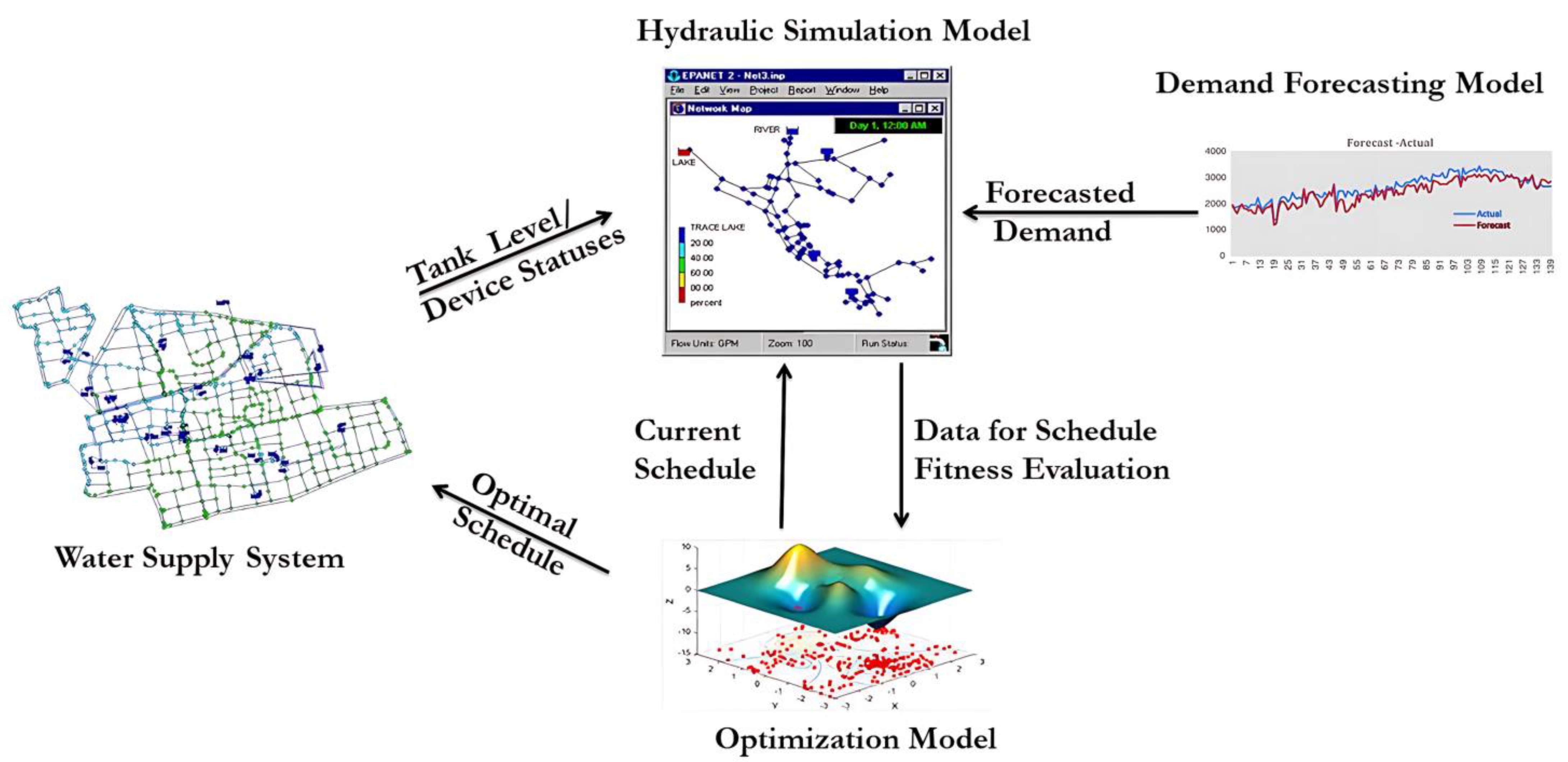
Taking into account the complexity and computational challenges of operating and controlling WDSs in real-world operating practices, and given that integrated water and energy demand forecasting is highlighted as a priority research area in [25], this study proposes a handy approach for optimized near real-time operational control that proactively responds to short-term (e.g., every 15, 30, and 60 min) water demand variations, while attaining the energy minimization goal. The proposed framework combines (a) a water demand forecasting model, (b) a network-wide hydraulic model, and (c) an optimization-based control model. Features of the proposed model compared to the existing models include: (1) implementing a shorter time step-based operational control schedule to respond to the dynamic nature of WDSs; (2) jointly optimizing the schedules of varying-speed pumps and valve settings (open/closed/active); and (3) guaranteeing hydraulic continuity between different operational and control time steps by carrying forward the hydraulic statuses (tanks levels, pumps, and valve statuses) derived from actual water demands (as opposed to forecasted water demands) from the preceding time steps.

2. Materials and Methods

2.1. Real-Time Scheduling Framework

Figure 1 illustrates the real-time scheduling framework proposed in this study. This framework is based on the integration of the following three models: (a) water demand forecasting model, (b) real-time optimization model, and (c) hydraulic simulation model. For the first operational time step, the algorithm updates the hydraulic simulation model with the initial tank levels and forecasted nodal demands to determine the optimal pump speeds as a continuous variable and discrete valve statuses that will minimize the operational costs in the given time step. It is noteworthy that pump speeds and valve statuses are subject to tank level constraints that ensure the real-world practice of tank turnover on a 24 h horizon. The developed constraints will make sure the tanks are filled enough during peak hours, and account for unusual fluctuations that might occur to the tank level variations during the optimization of pump and valve settings. The actual hydraulic model is then executed in parallel using the optimal pump speeds and valve statuses, but with actual nodal demands.
It should be noted that the actual nodal demands could be different from the forecasted nodal demands that were used for determining the optimal pump and valve statuses. This variation in actual water demands is expected to inform the merit of the proposed real-time WDS control framework. The actual hydraulic status of the system at the end of each time step is carried forward into the simulation model to set the initial boundary conditions for determining the optimal control strategies in the next time step. This integrated computational model is used to generate the optimal WDS control settings for the horizon period, at one time step at a time. The individual computational models used in the proposed framework are further described in the following paragraphs.

2.1.1. Water Demand Forecasting Model

A water demand forecasting model that is capable of forecasting nodal demands for each operational time step based on past water demand data is developed using a shallow artificial neural networks algorithm in MATLAB’s neural network toolbox. Nodal demands are forecasted one operational time step ahead, and passed on to the optimization model for determining the optimal WDS control settings in the concerned time step. For lack of past real-world water demand data, a synthetic water demand generation function, represented by Equation (1), is used for demonstration purposes to generate historical water demand data for all time steps, considering some random variation (±10%) from the base water demand pattern. The hourly pattern of the base water demands of the benchmark WDS that is used for demonstration purposes in this study is adopted and modified accordingly based on the literature [26]. The water demand pattern (pi,t) values for the dynamic analysis time steps (i.e., 60, 30, and 15 min) will vary within ±5% of the hourly base water demand (qi) values.
D i , t = q i × p i , t × σ
where, D i , t is the generated synthetic past water demand for demand node i, at time step t of the day; q i is the hourly base water demand of node i; p i , t is the water demand pattern value of node i at time step t; and σ is the random variation introduced into the generator function (varying between 0.95 and 1.05).
Using Equation (1), 1000 data sets (base water demands) for the operational horizon period of 24 h were generated and subsequently used to train the forecasting model. The “train” function in MATLAB’s neural network toolbox is used to train the cascade-forward neural network that includes a connection from the input and every previous layer to the following layers. Day of the week and time of day were used as inputs based on the time step number to train the forecasting model. The outputs were the forecasted water demands for all the demand nodes. The accuracy of the water demand forecasting model is measured using the mean absolute percentage error (MAPE), by comparing new water demand values generated using the water demand generator function with the forecasted values for the entire 24 h duration. MAPE values ranging from 5.2 to 8.8% were observed (for 60 min, 30 min, and 15 min time steps), showing acceptable accuracy of the water demand forecasting model.

2.1.2. Hydraulic Simulation Model

The hydraulic model used in this study is a computational experiment developed in the MATLAB interface based on the EPANET 2.0 simulation engine [27]. This model performs extended period simulations of the pressurized WDSs, and it is used for both simulation modeling (as part of the optimization framework) and actual hydraulic modeling (representing the actual WDS) purposes. In the optimization process, the hydraulic model is used to simulate the WDS at a given operational time step based on forecasted nodal demands to determine the best set of control strategies. In actual WDS modeling, the hydraulic model is used to mimic the actual WDS behavior in the same operational time step based on actual nodal demands (i.e., generated using Equation (1)) under the control strategies determined from the optimization model. The objective of the optimization algorithm is to minimize the total energy cost, which is derived from the actual WDS hydraulic model. To guarantee hydraulic continuity between consecutive operational time steps, component statuses (tank levels, pump speeds, and valve statuses) at the end of the actual WDS simulation time step are carried forward to the beginning of the next time step in both optimization and actual WDS simulation models.

2.1.3. Control-Based Optimization Model

A genetic algorithm (GA)-based optimization model is used in this study for developing near real-time control strategies for WDSs. GA-based methods are reported to be robust for optimizing WDS characteristics (e.g., pipe sizes, tank sizes, and pump sizes and schedules) as they can handle discrete variables efficiently to produce a set of promising results [28]. An EPANET-MATLAB Toolkit [29] associated with a single-objective genetic algorithm in the MATLAB programming environment is employed to determine optimal pump and valve schedules that minimize the total operational energy costs for the operational horizon period of 24 h. Multiple optimization runs with a population size of 100 and 200 generations are carried out. Pumps were considered to have constant efficiency of 75% and continuous pump speed values between 0 and 1.25, which correspond to pump speeds of zero (pump is “off”) up to when the pump speed is 1.25, as high as the baseline speed. The hydraulic simulation has been set to penalize the values of pump speed that are so low that they might cause backflow. The PRVs were considered to have “active,” “open,” and “closed” statuses in any operational time step. Active status means the PRV is partially opened to constrain downstream pressure to its pressure setting when the upstream pressure is higher than the setting. The PRV will be fully open if the upstream pressure is below the setting, and closed if the pressure on the downstream side exceeds that on the upstream side (i.e., reverse flow is not allowed) [27]. A penalty function is added to the optimization algorithm to penalize candidate solutions that produce nodal pressures less than the minimum required (which is considered to be 40 psi in normal operation for the benchmark WDS) for any demand node. Additionally, a comprehensive set of constraints were designed to control the tank levels. They account for (1) maintaining the minimum and maximum thresholds of the tank levels that equal the same values from the baseline according to Table 1, (2) determining the consistent filling or drafting mode of the tank for continuous time steps by assigning a value of zero and one to avoid unwanted fluctuations, and (3) attempting to keep tank levels at their highest during peak hours. Additionally, a boundary condition was set to restrict the initial values of pump speeds according to the previous time step entries so as to avoid outlying solutions.
Minimum tank levels are shown to be a good measure of supply reliability in water distribution systems [19]. The minimum tank level in this study is defined as the level of water that remains untouched during operation to overcome any contingencies (significant demand volume differences) that might arise in the system. Meeting minimum pressure and water tank level constraints are assumed to maintain acceptable system reliability. Finally, the end tank level is constrained to be within 15% of the initial tank level. The operational cost (OC) is calculated based on the pump energy consumed in each operational time step. The pump energy costs were considered, as they account for most of the operational costs over the lifecycle. A flat electricity rate is used, considering USD 0.12/kWh [30] of electricity cost aggregated for the operational horizon (24 h). In the proposed operational control framework, the optimization takes place for only one time step at a time, and the result of this time step will not have any bearing on the optimization process of the next time step. The optimization scheme does not have continuity, and therefore a time of use (TOU) power tariff rate was not employed.

2.2. Study Methodology

For demonstration purposes, two types of operational schemes were simulated, and their results were compared. Firstly, a conventional rule-based operational scheme (hereafter “baseline”) is simulated, in which the pump control decisions (switches) are only dependent on the tank levels (baseline scenario). In this scheme, constant-speed pumps operate following the predetermined rules that are obtained from the literature for the chosen benchmark WDS, as shown in Table 1. Specifically, their static, binary status of “ON” (the pump’s normal operational speed) and “OFF” is determined based on the critical tank levels according to Table 1. In the second scheme, a near real-time control model is used to generate pump speeds and valve schedules for the next operational time step based on the prevailing system conditions up until the current operational time step, by factoring in a comprehensive set of tank constraints. In this second type of operational scheme, three dynamic analysis time steps—60, 30, and 15 min—are compared to the hourly baseline scenario.

2.3. Demonstration

A small-sized benchmark WDS, depicted in Figure 2, which was originally proposed by [13], is used for demonstrating the proposed near real-time WDS control framework.
The chosen benchmark WDS (hereafter BWDS) comprises 126 nodes, 1 constant head source, 2 tanks, 168 pipes, 2 pumps, and 8 valves, and is subjected to normal water demand loading. An operational horizon of 24 h is considered in this study. BWDS is a real WDS that was twisted to preserve its anonymity. The network features are further modified in this study by adding 2.27 m 3 / h of water demand at each node, and modifying the water demand pattern to have no less than 20% (0.2 multipliers) of the base water demand at any time during the 24 h operational horizon (at night usually). These modifications were made to avoid negative values in the water demand forecasting model. The modified water demand pattern adopted from the literature is illustrated in Figure 3.
It is noteworthy that the baseline scheme, which is based on predetermined rule-based controls, is conservative and strives to maintain tank levels between tighter boundaries (as can be seen in Table 1). Similarly, the real-time control schemes are deliberately designed to follow the same rules of minimum and maximum levels to make them comparable to the baseline values.

3. Results and Discussion

3.1. Proposed Real-Time Scheduling Framework Performance

This section attempts to make a reasonable comparison between the model’s performance under different dynamic time steps and the conservative, static scenario where rules are predefined (i.e., the current practice at most water utilities). Table 2 summarizes the results from each operational scheme in terms of average operational cost over the 24 h horizon period. As expected, a shorter time step duration of 15 min led to more energy-friendly control of WDS operations based on operational costs. Operational efficacy is defined in this study as the capability of a WDS to deliver service to its customers in the most cost-effective manner possible, while still ensuring the acceptable quality of its service by maintaining minimum pressures at the demand nodes and tanks. It can be seen from Table 2 that a 60 min operational time step in the dynamic analysis resulted in about 17.1% savings in operational costs compared to the baseline scenario, followed by 17.4% for 30 min, and 17.8% for 15 min operational time steps. These savings could be more for larger WDSs. The average computational time needed to complete the control-based optimization for the shortest time step of 15 min duration (which is the most computationally intensive) was found to be less than 11 min in this study when used on a cluster using parallel computing. This is an important consideration for realizing the near real-time control vision, as the computational time cannot exceed the operational time step duration.
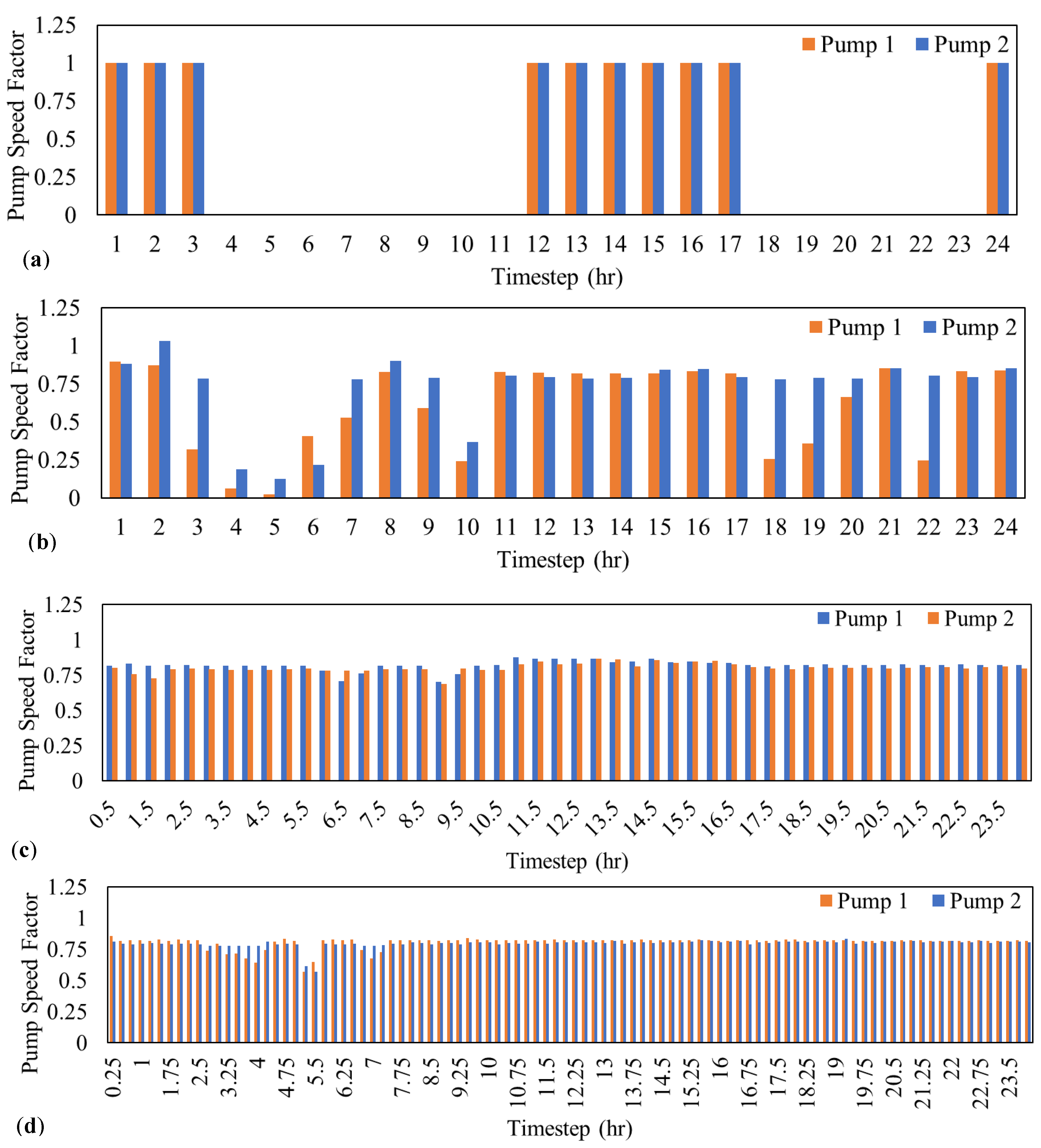
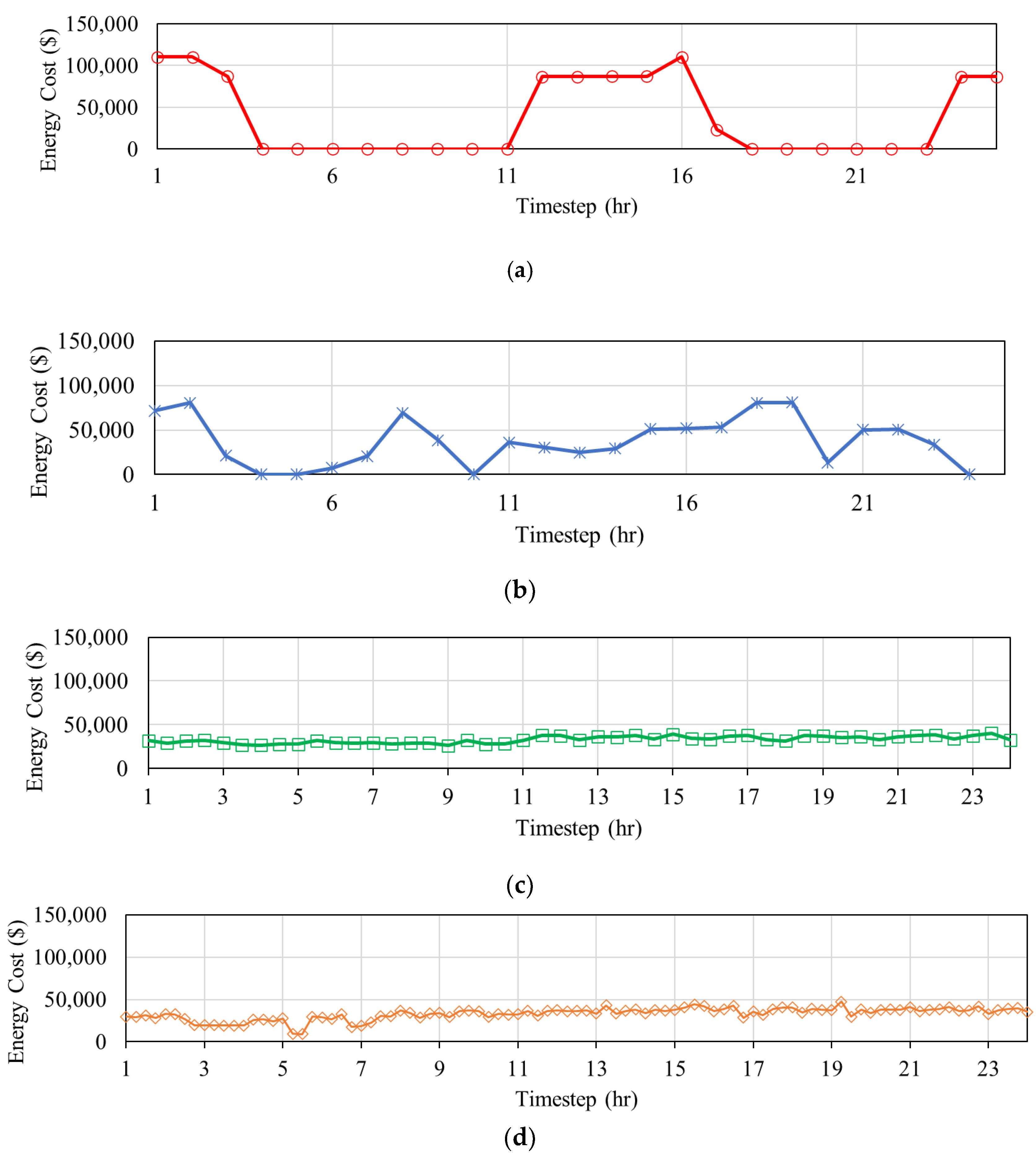
Figure 4 illustrates the schedules of both pumps for all the control schemes. Additionally, the pump energy profile over the 24 h horizon for all time steps is provided in Figure 5 to illustrate the kind of solutions the real-time control method produced.
The following points provide insights into why the optimal real-time scheme minimized energy consumption compared to the baseline scheme:
  • In the real-time scheme, energy consumption reduction is achieved by having the operational speed of pumps and valves vary compared to the conservative baseline scenario operations of tanks and pumps, where the criterion for operating a pump is solely based on whether a tank has reached its minimum or maximum level. However, the range within which tank levels can vary remains similar in real-time, dynamic operations to make the scenarios more comparable. One practical reason for the energy reduction is associated with the reduction in the speed, and thus the energy, of the pumps, which sets the priority on energy conservation rather than filling up the tanks suboptimally using pumps running at higher speeds. However, there are other plausible factors contributing to energy conservation, such as dynamic controls of valve settings. According to 
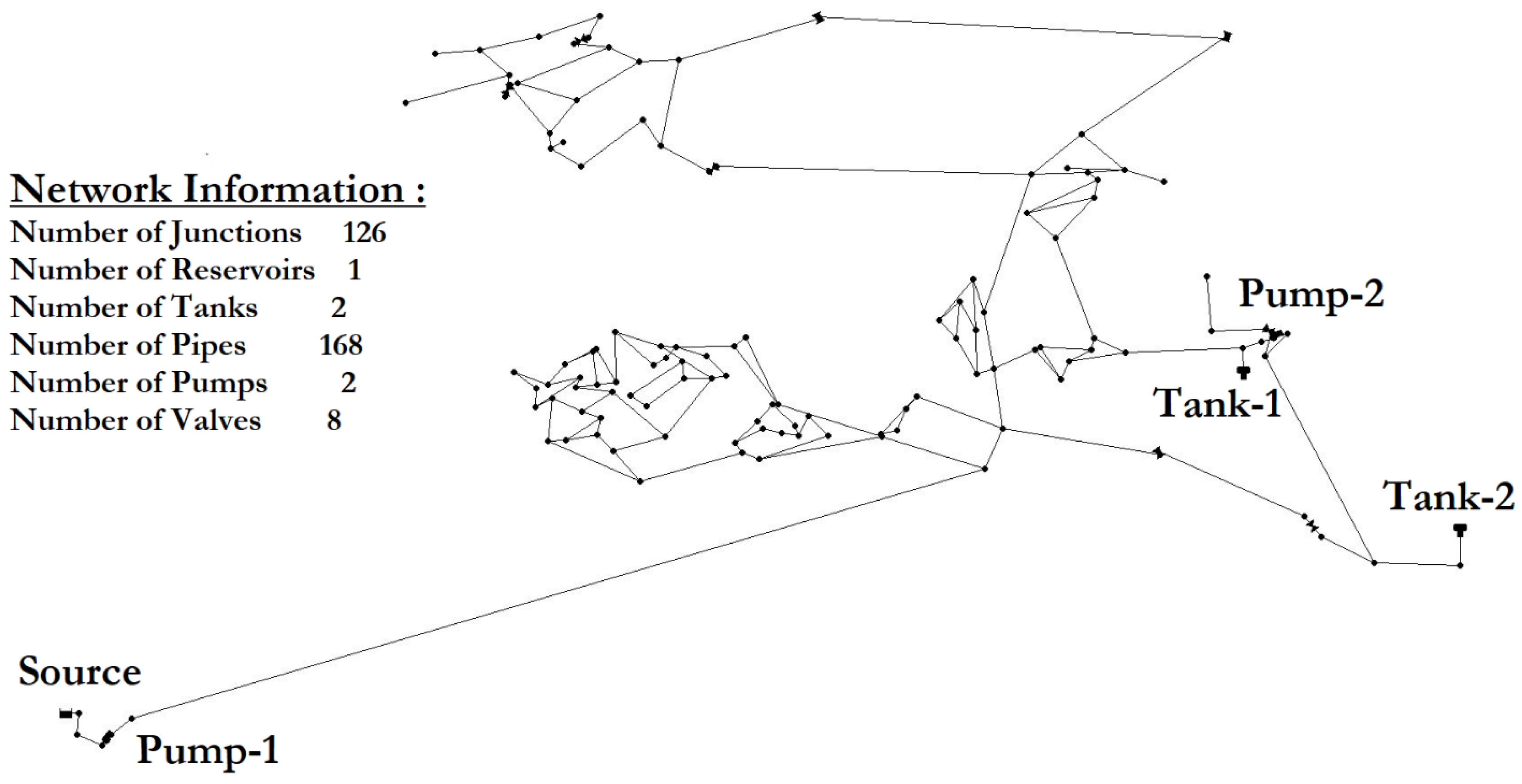
Figure 2, some of the valves are strategically located, in that they can alter pressure zone boundaries, and thus the dynamic controls of their settings can contribute to the reduction in the overall system pressure and, hence, the less consumed energy;
  • Because the objective in the real-time operation is energy conservation, the tank levels have to follow the optimization purpose, and the observation associated with it turns out to be more numbers of fill/draft trends compared to the baseline scenario;
  • The number of pump switches is not a critical issue, as the pumps undergo speed variations rather than the operationally expensive fact of being “on” or “off”; this means that the pumps experience less friction, fewer constant on/off changes, and thus experience a higher lifespan in the long run.
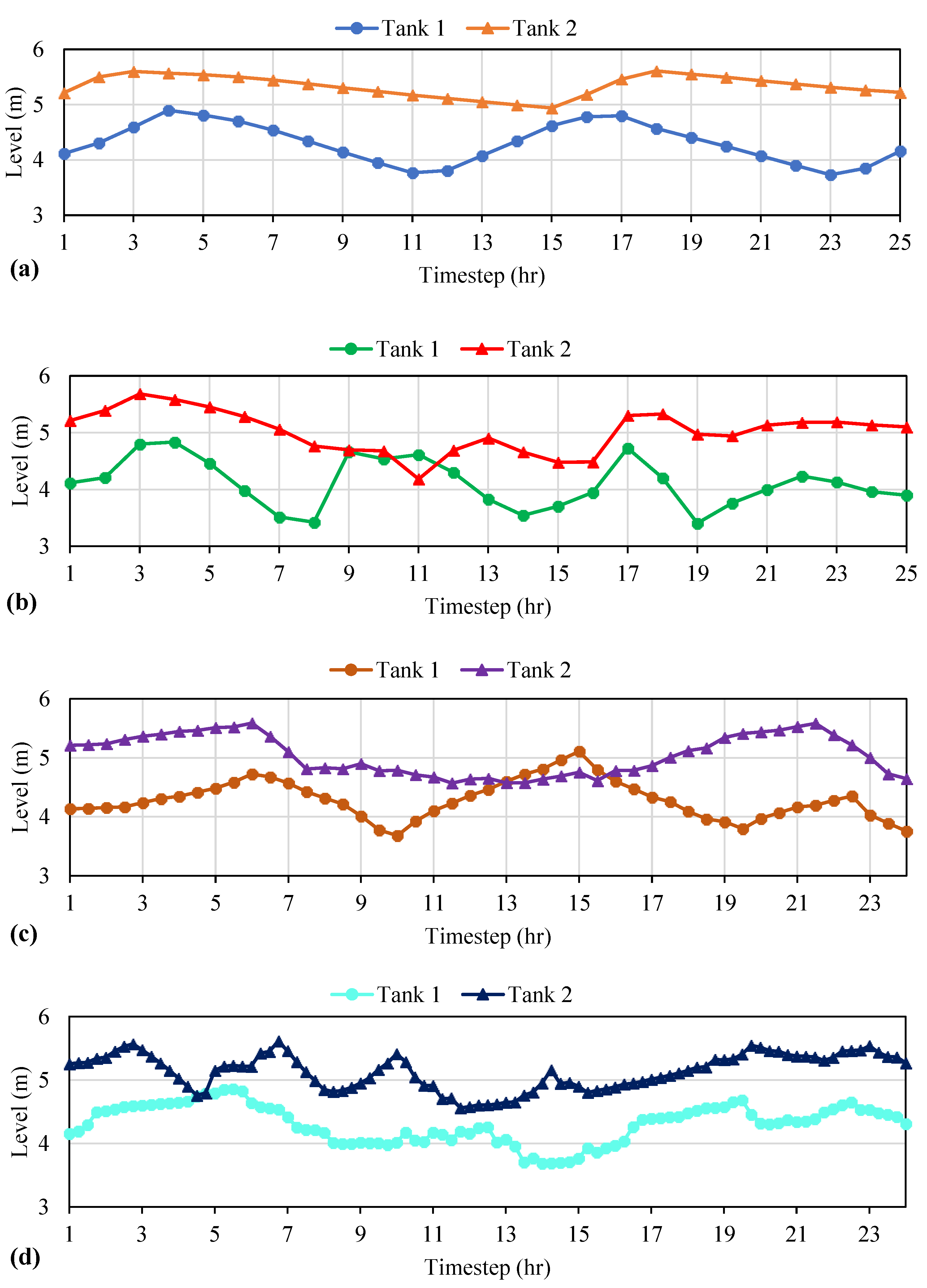
Tank levels for both optimized and baseline schemes over the operational horizon are presented below in Figure 6. It can be seen that tanks are constrained to run a normal turnover throughout the 24 h horizon for all scenarios. One notable observation is the fact that tanks undergo more cycles of filling and drafting in the real-time scenarios compared to the baseline scenario, which suggests that when pumps are running at lower speeds, tanks play a more significant role than in the baseline scheme.

3.2. Sensitivity Analyses

Sensitivity analyses were conducted to investigate the sensitivity of the proposed near real-time control framework to variation in certain critical model parameters. The sensitivity analysis parameters of interest to be evaluated toward the energy cost in the proposed model are (1) the percentage of actual water demand variation (σ) and (2) minimum tank levels. These parameters are selected based on their importance in operational practices and potential influence on costs and WDS control strategies. All operational time step durations in this study (i.e., 60 min, 30 min, and 15 min) are considered for conducting all the sensitivity analyses using three runs for each analysis. The purpose of this sensitivity analysis is not only to test the robustness of the model under different operational circumstances, but also to compare the model’s performance under the three dynamic time steps to draw inferences as to whether shorter time steps result in better solutions.

3.2.1. Actual Water Demand Variation

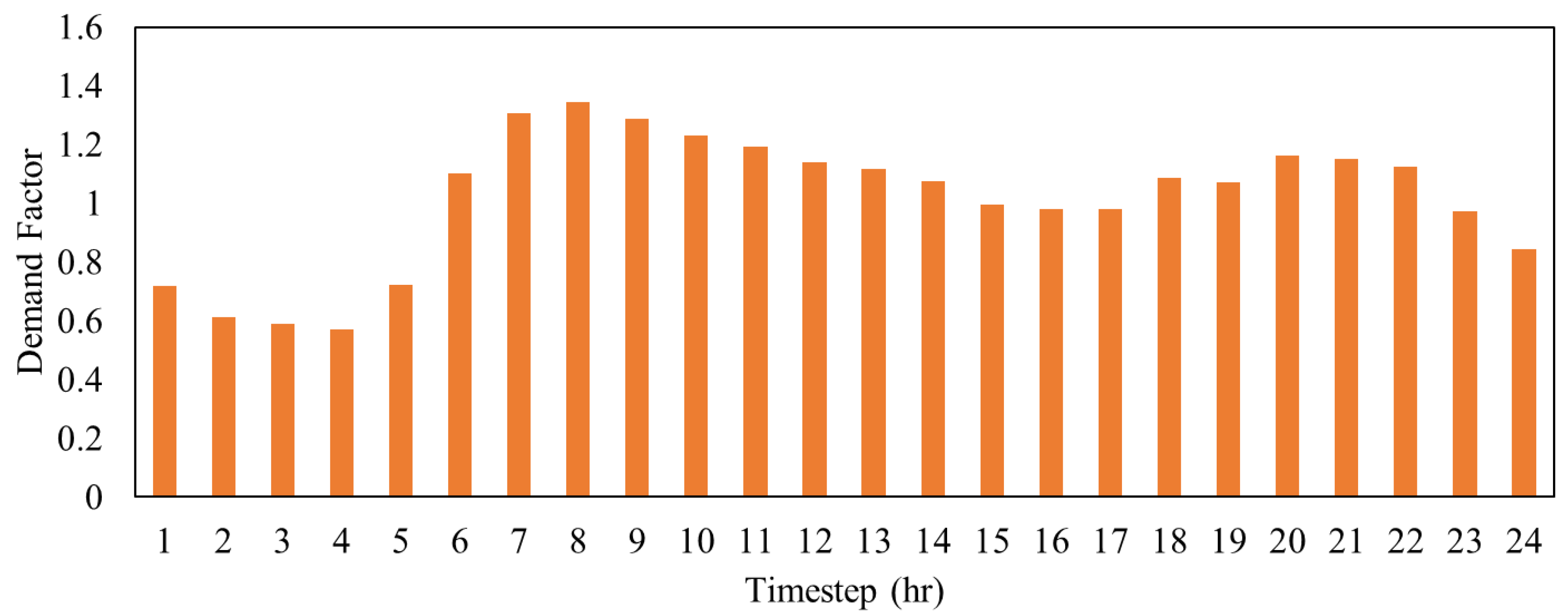
There is uncertainty associated with nodal water demands. This uncertainty has been characterized in this study using ±5% variation compared to the hourly base water demand pattern, as presented in Equation (1). This variation was considered in both past synthetic water demand data that was used in the water demand forecast model, and in the actual nodal demand generation during the hydraulic modeling in this study. The sensitivity of the results from the proposed framework to the variation in the water demand uncertainty is evaluated in this scenario. The water demand variation of ±1% and ±15% are considered in this scenario, while the default scenario considered ±5% variation. Table 3 illustrates the energy consumption cost, as well as the relative improvement in energy conservation in all dynamic time steps.
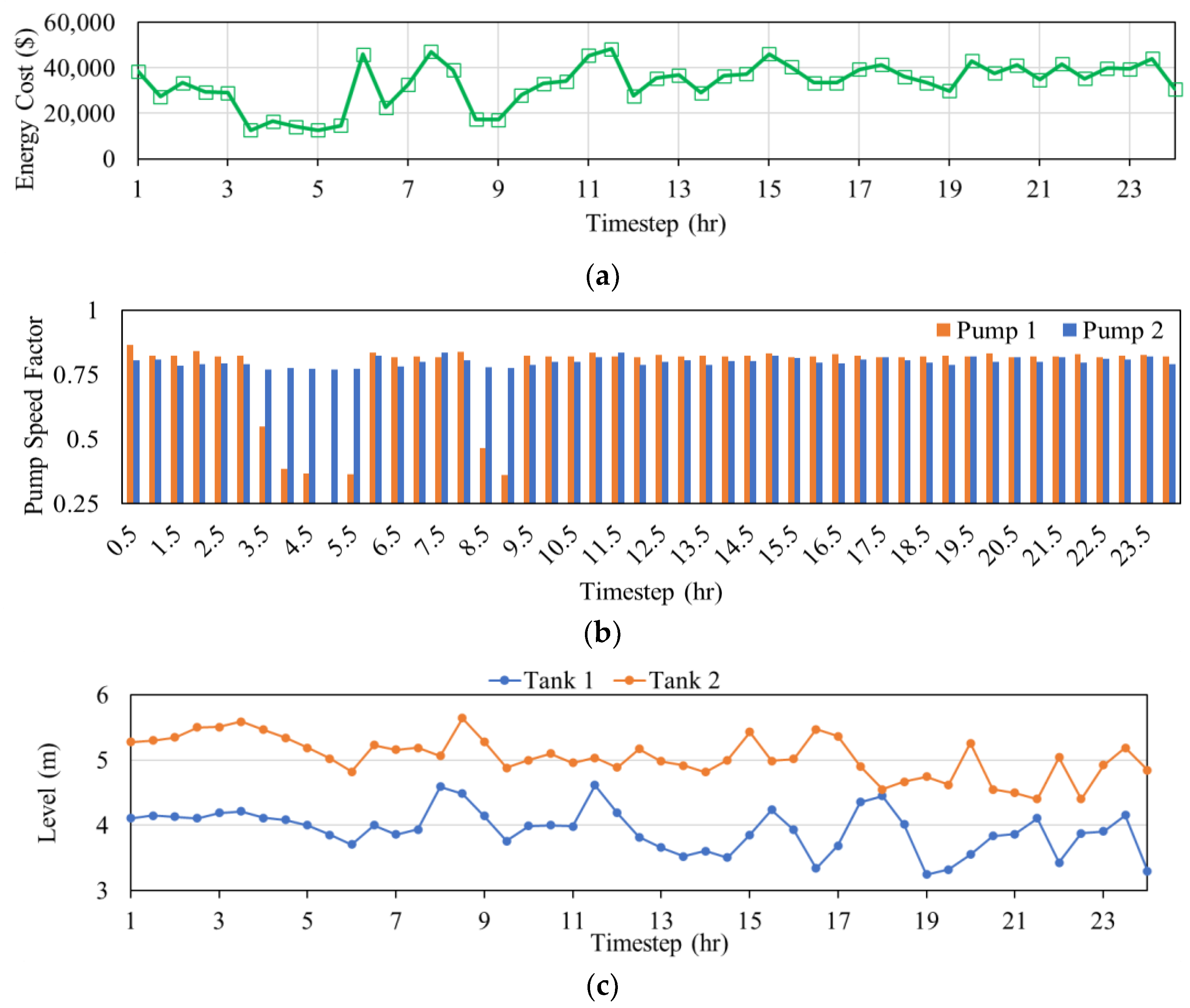
The relative improvements (savings) are associated with the baseline value of the corresponding conventional or real-time scenario. As opposed to the real-time scheme, the conventional method relies on fixed pattern-based demand data; therefore, no dynamic water demand variations are applied in its sensitivity analyses. Accordingly, no significant variations in the operational costs were observed from the results between either of the considered water demand-varied scenarios (i.e., ±15% and ±1%). To showcase a scenario granularly, the ±15% case for the 30 min time step has been depicted in Figure 7 in terms of operational features. The variations are not much different from those in the dynamic baseline scenario in terms of pump speed factor, tank levels, and energy variations for the 30 min case. Furthermore, according to Table 3, the ±15% and ±1% scenarios resulted in total energy consumption of roughly within −4% and 1%, respectively, compared to those conservative-scenario values of each time step in Table 2. This observed lack of sensitivity of the real-time control scheme to water demand variation of up to 15% is likely because the majority of the nodal demands in the BWDN are small (<6.81 m 3 / h ), and variation of up to 15% of these water demands may not have affected the system stability to require more pumping. Furthermore, even if the system stability is affected to a certain extent, tanks can be better used in the real-time scheme to meet higher water demands without having to turn on the pumps. Additionally, the energy consumption does not show significant improvements for different dynamic time steps.

3.2.2. Minimum Allowed Tank Levels

The minimum allowed tank level constraints (derived from the rule-based, conservative scenario) are varied in this scenario to investigate the sensitivity of the results to these parameters. There are two different-sized tanks in the BWDS with a diameter of 56.7 m and 32.3 m, and heights of 32.1 m and 9.8 m, respectively. Minimum allowed tank levels variation was investigated by increasing and decreasing them by one foot (0.305 m) compared to the two tank levels used in the default scenario. Table 3 demonstrates the effects of the minimum allowed tank levels’ variations on the energy consumption in the conservative vs. dynamic scenarios. As can be observed, relaxing the minimum tank level constraint lowers the energy consumption, whereas tightening the tank level constraint brings about more energy consumption in both the conservative and dynamic approaches. However, according to Table 3, the conservative approach is much more sensitive to the variations in the allowed minimum tank levels than the dynamic method. The relative savings in the conventional scenario are within a double-digit percentage (13.3% for lowering the tank level constraint by 0.305 m, and −20.5% for increasing the minimum tank level by 0.305 m), whereas those in the dynamic approach for all considered time steps vary within shortly above 1%. Specifically, as can be observed from the results presented in Table 3, when the minimum tank level constraint increased by 0.305 m, the operational cost in the real-time scheme marginally increased by 1.02%. On the other hand, relaxing constraints by reducing the minimum tank levels by 0.305 m produced lower operational costs, with savings of up to 0.45%. It is noteworthy that there is no linear correlation between the minimum tank levels and energy consumption, but it is found that, as a rule of thumb, increasing the minimum tank levels will increase the energy consumption, and decreasing them will reduce the system energy consumption in all dynamic time steps. Overall, it is fair to state that the dynamic approach shows more resistance than the conservative scenario to maintain a certain level of energy consumption amid variations in the minimum allowed tank levels. This may, in turn, be due both to the dynamicity of pump operations as opposed to flicking them on or off at different time steps, and to the real-time controls of valves that regulate the energy supply more consistently at each time step.
Although tank levels have some direct relation with pump operations, as elevated tanks could use available storage (buffer) to supply the WDS demand and reduce the pump operation times, the system can consume more energy to fill the tanks back up in case the minimum tank levels are lowered. It also applies to the scenario when less energy is required to fill the tanks back up when the minimum tank levels are increased; therefore, the variations of minimum tank levels are found to be slightly impacting the energy consumption in direct relation. There are more increments in cost amid increased allowable minimum tank levels when the dynamic time step is reduced from 60 to 15 min intervals, according to Table 3. This suggests the existence of more volatility and flexibility in the meta-heuristic optimization model when predicting the next time step.
In the sensitivity analysis section, it was observed that the real-time dynamicity (as opposed to predefined static rules) of operating system components plays a more significant role than merely reducing the time step from 60 min to 15 min. The variations in the parametric assumptions affect the energy consumption much less in the dynamic scenario and more in the conservative scenario.

3.3. Future Work and Limitations

Despite much research in the field of real-time control, it has not evolved enough for water utility practitioners to embrace its various aspects in practice. Multiple practical demonstrations of these approaches need to be undertaken before the experimental or computational research could yield much direct impact [6].
This study focused on ensuring that the computational time is shorter than the hydraulic time step. For real-time control, the computational time depends on the network size and, to some extent, on the number of sources, tanks, and other components. Still, the authors believe that the computational time can be shorter than a 15 min operational time step, even for very large networks, using the presented approach. The hydraulic simulation can be replaced with a trained neural network with reasonably high accuracy and considerable computational time savings. This claim needs to be validated in future research, and the proposed methodology should be tested with a large real-life WDS with multiple sources, pumps, and tanks to validate its merits. In addition, an extreme demand pattern (peak demand loading) was considered, along with contingency tank storage (minimum tank level) in this study, as reliability measures of WDSs; however, future work needs to address the sensitivity of the proposed approach to unusual and extraordinary events or demand loading, as well as uncertainties in large WDS networks.
Additionally, a multiobjective optimization model could be used to improve the scheduling framework by maximizing the operational resilience as an additional proposed objective that will provide the utility operator with a set of strategies to choose from, depending on how resilient the system is desired to be during potential failures. Another way to upgrade the framework would be adding more constraints to the single objective model, such as minimizing the number of pump switches and minimum operational resilience to keep the advantage of obtaining single optimal settings for each time step, especially in the case of automated operational control management. Additionally, the proposed control framework could be extended to achieve other system-level goals, such as leakage minimization and water quality control. Lastly, future work might include studying the relationship between pumping, tank level variation, water quality, and leakage in order to upgrade the WDS operation practices.
There are limitations of this study that may be addressed in the future. Firstly, the exclusion of real-world energy pricing considerations, such as time-of-day pricing and peak energy demand charges, when estimating the pumps’ operation cost. In future work, it is possible to adapt the proposed approach to include a hybrid control scheme, where the optimization also considers the operational horizon to attempt to minimize the cost based on a time of use (TOU) energy pricing scheme. Secondly, in this study, a constant efficiency of 75% was assumed for the pumps over the full range of operating conditions, which ignored the fact that pump efficiency varies with the flow.

4. Conclusions

A framework for optimized near real-time scheduling for the operation and control of WDSs is proposed and demonstrated in this paper. The operation and speed of pressure-reducing valves (PRVs) and pumps are jointly controlled based on an evolutionary optimization algorithm that is driven by near real-time system monitoring data (e.g., the system’s hydraulic data, tank level, etc.). Energy minimization is considered to be the goal while maintaining minimum pressure and minimum tank levels, as well as real-world tank level considerations as constraints. Dynamic operational control time steps of 60, 30, and 15 min are investigated and compared to the conventional hourly rule-based control for a small-sized WDS benchmark. The results revealed that real-time control schemes reduce the operational costs of the selected WDS between 17.1% and 17.8%, with the shortest time step scheme (15 min) offering the most reduction in operational expenses, at the cost of more computational expensiveness. Furthermore, the sensitivity analyses conducted on the single benchmark water distribution system revealed that the real-time control scheme was not greatly sensitive to the incremental changes in minimum tank levels or actual water demand variations. However, the findings suggested a somewhat direct correlation between minimum tank levels and energy conservation. Moreover, the system’s actual water demand variations due to the uncertainty in the system were found to play an insignificant role in the presented energy conservation scheme. It was also observed that shifting from static, conservative operations of components in a water distribution system to a real-time, dynamic approach provides more energy conservation, real-time knowledge of the system, and thus more flexibility and awareness to interact with the system than merely reducing the time steps to minutes. Lastly, it was found that the average computational time for each run in the shortest real-time control time step of 15 min is less than 11 min, if run on cluster parallel computing nodes.

Author Contributions

Conceptualization, A.A.B.M.; methodology, A.A.B.M.; software, A.A.B.M. and A.M.; validation, A.M.; formal analysis, A.A.B.M.; data curation, A.M.; writing—original draft, A.A.B.M.; writing—review and editing, A.M. and K.R.P.; visualization, A.M.; supervision, K.R.P. All authors have read and agreed to the published version of the manuscript.

Funding

The authors are thankful to King Saud University, Riyadh, Saudi Arabia, for supporting this research study through the Researchers Supporting Project number (RSP2023R302). This research was also partly supported by the National Science Foundation (NSF) under Grant No. 1638321 and No. 1745300. The views and conclusions contained in this document are those of the authors and should not be interpreted as necessarily representing the official policies, either expressed or implied, of the United States Government. The support of the NSF is greatly appreciated.

Institutional Review Board Statement

Not applicable.

Informed Consent Statement

Not applicable.

Data Availability Statement

Data are available from the corresponding author upon reasonable request.

Acknowledgments

The authors extend their appreciation to the Researchers Supporting Project number (RSP2023R302), King Saud University, Riyadh, Saudi Arabia, for funding this work.

Conflicts of Interest

The authors declare no conflict of interest.

References

  1. ASCE. Committee on America’s Infrastructure. 2021 Infrastructure Report Card; American Society of Civil Engineers: Reston, VA, USA, 2021. [Google Scholar]
  2. Bello, O.; Abu-Mahfouz, A.M.; Hamam, Y.; Page, P.R.; Adedeji, K.B.; Piller, O. Solving Management Problems in Water Distribution Networks: A Survey of Approaches and Mathematical Models. Water 2019, 11, 562. [Google Scholar] [CrossRef] [Green Version]
  3. USEPA. Ensuring a Sustainable Future: An Energy Management Guidebook for Wastewater and Water Utilities, Office of Wastewater Management Contract Number GS-10F-0337M (Issue January). National Service Center for Environmental Publications (NSCEP). 2008. Available online: https://www3.epa.gov/npdes/pubs/pretreatment_ensuring_sustainable_future.pdf (accessed on 21 February 2023).
  4. Smith, R.; Goldstein, W. Water and Sustainability: U.S. Electricity Consumption for Water Supply & Treatment—The Next Half Century; Electric Power Research Institute, Inc. (EPRI): Washington, DC, USA, 2002; Volume 4. [Google Scholar]
  5. Ormsbee, L.; Lingireddy, S.; Chase, D. Optimal pump scheduling for water distribution systems. In Proceedings of the Multidisciplinary International Conference on Scheduling: Theory and Applications (MISTA 2009), Dublin, Ireland, 10–12 August 2009; pp. 10–12. [Google Scholar]
  6. Creaco, E.; Campisano, A.; Fontana, N.; Marini, G.; Page, P.R.; Walski, T. Real time control of water distribution networks: A state-of-the-art review. Water Res. 2019, 161, 517–530. [Google Scholar] [CrossRef] [PubMed]
  7. Price, E.; Ostfeld, A. Discrete Pump Scheduling and Leakage Control Using Linear Programming for Optimal Operation of Water Distribution Systems. J. Hydraul. Eng. 2014, 140. [Google Scholar] [CrossRef]
  8. Yu, G.; Powell, R.S.; Sterling, M.J.H. Optimized pump scheduling in water distribution systems. J. Optim. Theory Appl. 1994, 83, 463–488. [Google Scholar] [CrossRef]
  9. Goldman, F.E.; Mays, L.W. The Application of Simulated Annealing to the Optimal Operation of Water Systems. In Proceedings of the WRPMD’99 Preparing for the 21st Century, Tempe, AZ, USA, 6–9 June 1999. [Google Scholar] [CrossRef] [Green Version]
  10. Mackle, G.; Savic, G.A.; Walters, G.A. Application of genetic algorithms to pump scheduling for water supply. In Proceedings of the 1st International Conference on Genetic Algorithms in Engineering Systems: Innovations and Applications (GALESIA), Sheffield, UK, 12–14 September 1995; Institution of Engineering and Technology (IET): Stevenage, UK, 1995; Volume 1995, pp. 400–405. [Google Scholar]
  11. Mahmoud, A.A.B.; Piratla, K.R. Optimal Operational Control of Water Pipeline Systems Using Real-Time Scheduling Framework. In Pipelines 2019: Planning and Design; American Society of Civil Engineers: Reston, VA, USA, 2019; pp. 243–248. [Google Scholar]
  12. López-Ibáñez, M.; Prasad, T.D.; Paechter, B. Ant Colony Optimization for Optimal Control of Pumps in Water Distribution Networks. J. Water Resour. Plan. Manag. 2008, 134, 337–346. [Google Scholar] [CrossRef]
  13. Ostfeld, A.; Tubaltzev, A. Ant Colony Optimization for Least-Cost Design and Operation of Pumping Water Distribution Systems. J. Water Resour. Plan. Manag. 2008, 134, 107–118. [Google Scholar] [CrossRef]
  14. Giacomello, C.; Kapelan, Z.; Nicolini, M. Fast Hybrid Optimization Method for Effective Pump Scheduling. J. Water Resour. Plan. Manag. 2013, 139, 175–183. [Google Scholar] [CrossRef]
  15. Krapivka, A.; Ostfeld, A. Coupled Genetic Algorithm—Linear Programming Scheme for Least-Cost Pipe Sizing of Water-Distribution Systems. J. Water Resour. Plan. Manag. 2009, 135, 298–302. [Google Scholar] [CrossRef]
  16. Campisano, A.; Modica, C.; Reitano, S.; Ugarelli, R.; Bagherian, S. Field-Oriented Methodology for Real-Time Pressure Control to Reduce Leakage in Water Distribution Networks. J. Water Resour. Plan. Manag. 2016, 142, 04016057. [Google Scholar] [CrossRef]
  17. Brentan, B.; Meirelles, G.; Luvizotto, E., Jr.; Izquierdo, J. Joint Operation of Pressure-Reducing Valves and Pumps for Improving the Efficiency of Water Distribution Systems. J. Water Resour. Plan. Manag. 2018, 144, 04018055. [Google Scholar] [CrossRef] [Green Version]
  18. Kang, D. Real-time Optimal Control of Water Distribution Systems. Procedia Eng. 2014, 70, 917–923. [Google Scholar] [CrossRef] [Green Version]
  19. Odan, F.K.; Reis, L.F.R.; Kapelan, Z. Real-Time Multiobjective Optimization of Operation of Water Supply Systems. J. Water Resour. Plan. Manag. 2015, 141, 04015011. [Google Scholar] [CrossRef]
  20. Odan, F.K.; Reis, L.F.R. Hybrid Water Demand Forecasting Model Associating Artificial Neural Network with Fourier Series. In Proceedings of the 12th Annual Conference on Water Distribution Systems Analysis (WDSA), Tucson, AN, USA, 12–15 September 2010; pp. 1287–1305. [Google Scholar] [CrossRef] [Green Version]
  21. Mala-Jetmarova, H.; Sultanova, N.; Savic, D. Lost in optimisation of water distribution systems? A literature review of system operation. Environ. Model. Softw. 2017, 93, 209–254. [Google Scholar] [CrossRef] [Green Version]
  22. Alvisi, S.; Franchini, M.; Marinelli, A. A short-term, pattern-based model for water-demand forecasting. J. Hydroinformatics 2007, 9, 39–50. [Google Scholar] [CrossRef] [Green Version]
  23. Salomons, E.; Housh, M. A Practical Optimization Scheme for Real-Time Operation of Water Distribution Systems. J. Water Resour. Plan. Manag. 2020, 146, 04020016. [Google Scholar] [CrossRef]
  24. Rao, Z.; Salomons, E. Development of a real-time, near-optimal control process for water-distribution networks. J. Hydroinformatics 2007, 9, 25–37. [Google Scholar] [CrossRef] [Green Version]
  25. Sowby, R.B. Making waves: Research to support water and wastewater utilities in the transition to a clean-energy future. Water Res. 2023, 233, 119739. [Google Scholar] [CrossRef] [PubMed]
  26. Marchi, A.; Salomons, E.; Ostfeld, A.; Kapelan, Z.; Simpson, A.R.; Zecchin, A.C.; Maier, H.R.; Wu, Z.Y.; Elsayed, S.M.; Song, Y.; et al. Battle of the Water Networks II. J. Water Resour. Plan. Manag. 2014, 140, 04014009. [Google Scholar] [CrossRef] [Green Version]
  27. Rossman, L.A. Epanet 2 users manual, us environmental protection agency. In Water Supply and Water Resources Division; National Risk Management Research Laboratory: Cincinnati, OH, USA, 2000; p. 45268. [Google Scholar]
  28. Prasad, T.D.; Park, N.-S. Multiobjective Genetic Algorithms for Design of Water Distribution Networks. J. Water Resour. Plan. Manag. 2004, 130, 73–82. [Google Scholar] [CrossRef]
  29. Eliades, D.G.; Kyriakou, M.; Vrachimis, S.G.; Polycarpou, M.M. EPANET-MATLAB Toolkit: An Open-Source Software for Interfacing EPANET with MATLAB. In Proceedings of the 14th International Conference on Computing and Control for the Water Industry (CCWI), Amsterdam, The Netherlands, 7–9 November 2016. [Google Scholar]
  30. Geem, Z.W. Harmony search optimisation to the pump-included water distribution network design. Civ. Eng. Environ. Syst. 2009, 26, 211–221. [Google Scholar] [CrossRef]
Figure 1. Proposed real-time scheduling framework.
Water 15 01280 g001
Figure 2. Layout of BWDS (adapted from [13]).
Water 15 01280 g002
Figure 3. Modified water demand pattern for BWDS (adapted from [26]).
Water 15 01280 g003
Figure 4. The two pump schedules over the operational horizon: (a) baseline, (b) 60 min, (c) 30 min, and (d) 15 min.
Water 15 01280 g004
Figure 5. Pump energy profile over the 24 hour operation period: (a) baseline, (b) 60 min, (c) 30 min, and (d) 15 min.
Water 15 01280 g005
Figure 6. Tank levels profile over the 24 hour operation period for (a) baseline, (b) 60 min, (c) 30 min, and (d) 15 min.
Water 15 01280 g006
Figure 7. Variations of (a) energy consumption, (b) pump speed, and (c) tank levels for sensitivity analysis of system water demand randomization within 15%.
Water 15 01280 g007
Table 1. Conventional rule-based (baseline) pump control scheme for BWDS.
Pump IDClose WhenOpen When
Pump-1Tank-1 water level > 5.2 mTank-1 water level < 4 m
Pump-2Tank-2 water level > 5.9 mTank-2 water level < 5 m
Table 2. Summary of results for different control schemes over a year.
SchemeAvg. Cost
(in USD 1000)
Avg. Saving %
BaselineUSD 962.27--
60 minUSD 798.5217.1%
30 minUSD 795.2217.4%
15 minUSD 791.6117.8%
Table 3. Sensitivity analysis results for actual water demand variations and minimum allowed tank level in conventional and dynamic time steps.
Parameter VariationsHourly Energy Consumption Cost (Conventional)Hourly Energy Consumption Cost (Real-Time)
60 min30 min15 min
AC 2RS 3ACRSACRSACRS
Baseline 1962.71--798.22--795.22--791.61--
Demand Variations within ±1%----796.790.17%803.00−0.98%790.040.20%
Demand Variations within ±15%----819.37−2.64%821.80−3.34%823.02−3.97%
Minimum Allowed Tank Level Variations minus 0.305 m835.0213.3%793.740.56%791.620.45%786.300.67%
Minimum Allowed Tank Level Variations plus 0.305 m1159.9−20.5%800.33−0.26%803.32−1.02%801.28−1.22%
Notes: 1 Actual baseline variation: within ±5% and baseline. Min: Tank-1 (4 m) and Tank-2 (5 m); initial: Tank-1 (4.6 m) and Tank-2 (5.4 m). 2 Average hourly cost over the 24 h operational horizon (in USD 1000). 3 Relative savings in percentage compared to the corresponding baseline value.
Disclaimer/Publisher’s Note: The statements, opinions and data contained in all publications are solely those of the individual author(s) and contributor(s) and not of MDPI and/or the editor(s). MDPI and/or the editor(s) disclaim responsibility for any injury to people or property resulting from any ideas, methods, instructions or products referred to in the content.

