Applying Linear Forms of Pseudo-Second-Order Kinetic Model for Feasibly Identifying Errors in the Initial Periods of Time-Dependent Adsorption Datasets

Abstract

Initial periods of adsorption kinetics play an important role in estimating the initial adsorption rate and rate constant of an adsorption process. Several adsorption processes rapidly occur, and the experimental data of adsorption kinetics under the initial periods can contain potential errors. The pseudo-second-order (PSO) kinetic model has been popularly applied in the field of adsorption. The use of the nonlinear optimization method to obtain the parameters of the PSO model can minimize error functions during modelling compared to the linear method. However, the nonlinear method has limitations in that it cannot directly recognize potential errors in the experimental points of time-dependent adsorption, especially under the initial periods. In this study, for the first time, the different linear types (Types 1–6) of the PSO model are applied to discover the error points under the initial periods. Results indicated that the fitting method using its linear equations (Types 2–5) is really helpful for identifying the error (doubtful) experimental points from the initial periods of adsorption kinetics. The imprecise points lead to low adjusted R² (adj-R²), high reduced χ² (red-χ²), and high Bayesian information criterion (BIC) values. After removing these points, the experimental data were adequately fitted with the PSO model. Statistical analyses demonstrated that the nonlinear method must be used for modelling the PSO model because its red-χ² and BIC were lower than the linear method. Type 1 has been extensively applied in the literature because of its very high adj-R² value (0.9999) and its excellent fitting to experimental points. However, its application should be limited because the potential errors from experimental points are not identified by this type. For comparison, the other kinetic models (i.e., pseudo-first-order, pseudo-nth-order, Avrami, and Elovich) are applied. The modelling result using the nonlinear forms of these models indicated that the fault experimental points from the initial periods were not detected in this study.

1. Introduction

Adsorption is a combination process (adsorption and desorption occur simultaneously) [1]. Adsorption kinetics is commonly conducted under batch experiments [2]. Some adsorption processes occur very fast. Guo et al. [3] found that the adsorption process of Cd²⁺ ions onto biosorbent (derived from maize straw modified with succinic anhydride) rapidly occurred under the first period of adsorption kinetics, with approximately 70.0–96.6% of total Cd²⁺ ion solutions (C_o = 100, 300, and 500 mg/L at pH = 5.8) being removed within 1 min. Zbair et al. [4] reported that the adsorption process of bisphenol A or diuron by Argan-nutshell-based hydrochar reached a fast equilibrium within 4 min of contact. An analogous result has been reported by many scholars who invested in the adsorption of Cd²⁺ ions onto orange-peel-derived biochar [5] and rhodamine B dye onto white-sugar-based activated carbon [6]. Therefore, some authors [3,5,6] took a very short time (1 min, 2 min, etc.) for adsorption kinetics instead of a longer one (i.e., starting from 10 min) [7].

Clearly, the initial periods of time-dependent adsorption datasets play an important role in establishing the adsorption rate constant and initial rate of adsorption kinetics. Hubbe et al. [8] called them “early” data points. However, some potential errors or technical mistakes can occur if samples are taken uncarefully and analysed for a very short time (i.e., 1 min, 2 min, etc.). The adsorption process often includes two phases: solid (material or adsorbent) and liquid. The liquid phase often contains solute (or adsorbate) and solvent (commonly water). In general, after withdrawing small fractions from the mixture of the solid and liquid at an interval of time, the liquid phase is separated from the mixture by the filtration or centrifugal method. A dilution step is additionally required if necessary. The available sites in a material can continue to adsorb adsorbate molecules in the withdrawn fractions if the separation process is delayed or not performed instantly. As a result, the concentrations of adsorbate at given times (C_t) decrease, and the amount of adsorbate adsorbed by an adsorbent at times (q_t) increases. This means that the values q_t at the initial periods might be higher than those expected if researchers do not conduct experiments carefully. They can be defined as the error points in datasets and affect the results of modelling adsorption on kinetics. It might be hard to verify those doubtful results by existing techniques, and this is a current limitation in this field.

In the study of kinetic adsorption, two common (reaction-called) models that are used to model time-dependent experiment data of the adsorption process are the pseudo-first-order (PFO) model and pseudo-second-order (PSO) model [9,10,11]. Lima et al. [2] concluded in their review that the PSO model describes most experimental data better than the PFO model. Some authors [12,13] indicated that the PSO model was initially established by Blanchard and co-workers [14] in 1984 to describe the time-dependent process of heavy metal adsorption by clinoptilolite. However, other authors [8] found that Coleman and co-workers [15] proposed a similar model earlier in 1956. Its differential equation is commonly expressed as Equation (1) [12]. After taking integration by applying the boundary conditions (q_t = 0 at t = 0, and q_t = q_t at t = t), the nonlinear form of the PSO model is obtained as Equation (2) [16].

$$\frac{d{q}_{\mathrm{t}}}{dt}=k_2(q_{\mathrm{e}(2)}-q_{\mathrm{t}}{)}^2$$

(1)

$$q_{\mathrm{t}}=\frac{q_{\mathrm{e}(2)}^2{k}_{2}t}{1+q_{\mathrm{e}(2)}{k}_{2}t}$$

(2)

$$q_{\mathrm{t}}=\frac{C_{\mathrm{o}}{-C}_{\mathrm{t}}}{m}\times V$$

(3)

where k₂ (kg/(mol × min)) is the rate constant of this model; q_e(2) and q_t (mol/kg) are the amounts of pollutant in the solution adsorbed by the material at equilibrium and any time t (min) is obtained from Equation (3); C_o and C_t (mol/L) are the concentrations of the pollutant at the beginning and any time t (min); m (kg) is the dry mass of the material; and V (L) is the volume of the pollutant used in the study of the adsorption kinetics.

Six types of linear forms of the PSO model are found in the literature [12,17,18,19]. Although Type 5 and Type 6 have been reported elsewhere [17,19], they are not commonly applied in the literature compared to Type 1. Type 1, which might have been introduced first by Ho and McKay [20], has been intensively applied in the literature because the R² or r² value obtained from this type is very close to 1 [2,12].

$$\frac{t}{q_{\mathrm{t}}}=(\frac{1}{q_{\mathrm{e}(2)}})t+\frac{1}{k_2{q}_{\mathrm{e}(2)}^2}(\mathrm{Type}1;\mathrm{the}\mathrm{plot}\mathrm{of}t/q_{\mathrm{t}}\mathit{vs}.t)$$

(4)

$$\frac{1}{q_{\mathrm{t}}}=(\frac{1}{k_2{q}_{\mathrm{e}(2)}^2})\frac{1}{t}+\frac{1}{q_{\mathrm{e}(2)}}(\mathrm{Type}2;\mathrm{the}\mathrm{plot}\mathrm{of}1/q_{\mathrm{t}}\mathit{vs}.1/t)$$

(5)

$$q_{\mathrm{t}}=\left(\frac{-1}{k_2{q}_{\mathrm{e}(2)}}\right)\frac{q_{\mathrm{t}}}{t}+q_{\mathrm{e}(2)}(\mathrm{Type}3;\mathrm{the}\mathrm{plot}\mathrm{of}{q}_{\mathrm{t}}\mathit{vs}.q_{\mathrm{t}}/t)$$

(6)

$$\frac{q_{\mathrm{t}}}{t}=-(k_2{q}_{\mathrm{e}(2)})q_{\mathrm{t}}+k_2{q}_{\mathrm{e}(2)}^2(\mathrm{Type}4;\mathrm{the}\mathrm{plot}\mathrm{of}{q}_{\mathrm{t}}/t\mathit{vs}.q_{\mathrm{t}})$$

(7)

$$\frac{1}{t}=k_2{q}_{\mathrm{e}(2)}^2\frac{1}{q_{\mathrm{t}}}-k_2{q}_{\mathrm{e}(2)}(\mathrm{Type}5;\mathrm{the}\mathrm{plot}\mathrm{of}1/t\mathit{vs}.1/q_{\mathrm{t}})$$

(8)

$$\frac{1}{\left(q_{\mathrm{e}(2)}-q_{\mathrm{t}}\right)}=k_{2}t+\frac{1}{q_{\mathrm{e}(2)}}(\mathrm{Type}6;\mathrm{the}\mathrm{plot}\mathrm{of}1/(q_{\mathrm{e}}-q_{\mathrm{t}})\mathit{vs}.t)$$

(9)

For comparison, several statistical analyses were applied along with the determination coefficient (R²; Equation (10)) and adjusted determination coefficient (adj-R²; Equation (11)). They include chi-squared (χ²; Equation (12)), reduced chi-square (red-χ²; Equation (13)), and Bayesian information criterion (BIC; Equation (14)) [2,12,16] A model with higher adj-R² value and lower red-χ² indicates a better fitting than the others. Because of the difference among the parameters of the models used, the magnitude (or the absolute value) of ΔBIC (BIC of model 1–BIC of model 2) is used for selecting the best fitting model [2,16].

$$R^2=\frac{\sum (y_{\mathrm{e}\mathrm{x}\mathrm{p}}-y_{\mathrm{e}\mathrm{x}\mathrm{p}-\mathrm{m}\mathrm{e}\mathrm{a}\mathrm{n}}{)}^2-\sum (y_{\mathrm{e}\mathrm{x}\mathrm{p}}-y_{\mathrm{m}\mathrm{o}\mathrm{d}\mathrm{e}\mathrm{l}}{)}^2}{\sum (y_{\mathrm{e}\mathrm{x}\mathrm{p}}-y_{\mathrm{e}\mathrm{x}\mathrm{p}-\mathrm{m}\mathrm{e}\mathrm{a}\mathrm{n}}{)}^2}=1-\frac{\sum (y_{\mathrm{e}\mathrm{x}\mathrm{p}}-y_{\mathrm{m}\mathrm{o}\mathrm{d}\mathrm{e}\mathrm{l}}{)}^2}{\sum (y_{\mathrm{e}\mathrm{x}\mathrm{p}}-y_{\mathrm{e}\mathrm{x}\mathrm{p}-\mathrm{m}\mathrm{e}\mathrm{a}\mathrm{n}}{)}^2}$$

(10)

$$\mathrm{a}\mathrm{d}\mathrm{j}-R^2=1-(1-R^2)\times (\frac{N-1}{\mathrm{D}\mathrm{O}\mathrm{F}})$$

(11)

$$\mathrm{r}\mathrm{e}\mathrm{d}-{\chi }^2=\frac{\sum (y_{\mathrm{e}\mathrm{x}\mathrm{p}}-y_{\mathrm{m}\mathrm{o}\mathrm{d}\mathrm{e}\mathrm{l}}{)}^2}{\mathrm{D}\mathrm{O}\mathrm{F}}$$

(12)

$$\mathrm{B}\mathrm{I}\mathrm{C}=N\times \mathrm{l}\mathrm{n}(\frac{\sum (y_{\mathrm{e}\mathrm{x}\mathrm{p}}-y_{\mathrm{m}\mathrm{o}\mathrm{d}\mathrm{e}\mathrm{l}}{)}^2}{N})+P\mathrm{l}\mathrm{n}(N)$$

(13)

where y_exp is q_t (mol/kg) obtained from experiments; y_exp–mean is an average of y_exp values used for modelling; y_model is q_t calculated based on the PSO model; N is the number of experimental points; P is the number of parameters of the model (I.e., P = 2 for the PSO model); and DOF is the degrees of freedom.

The nonlinear optimization method is often suggested to model the adsorption kinetic model because it can minimize error functions [1,2,12,16]. However, this method cannot provide information on potential errors in adsorption kinetic datasets. This study aimed to evaluate whether it is feasible to apply the linear forms of the pseudo-second-order kinetic model for feasibly identifying errors in the initial periods of kinetic adsorption. This hypothesis is introduced for the first time. The kinetic adsorption data were also fitted to some common models: the pseudo-first-order, pseudo-n^th-order, Avrami, and Elovich ones. Commercial activated carbon and paracetamol (PRC) were used as the target adsorbent and adsorbate.

2. Experimental Conditions and Procedures

The adsorption process of paracetamol (PRC, purchased from Sigma-Aldrich, St. Louis, MO, USA) using commercial activated carbon (CAC) was carried out. The surface area and total pore volume of CAC were 1275 m²/g and 0.670 cm³/g, respectively. The experiment of kinetics adsorption was conducted in triplicate, and the result of q_t was averaged. The adsorption condition was maintained at 25 °C, pH = 7.0, and initial PRC (3.45 mmol/L). The solutions (1.0 M NaOH and 1.0 M HCl) were used to adjust the pH of PRC solution before and during the adsorption process.

Approximately 1.0 g of CAC was added to an Erlenmeyer flask containing 1 L of PRC solution (3.45 mmol/L and pH = 7.0). The mixture of the solid/liquid was shaken at 150 rpm and 30 °C. The contact time range for studying adsorption kinetic was 1, 5, 15, 30, 45, 60, 90, 120, 180, 240, 300, 360, 720, 1440, 2880, and 4320 min (n = 16). After the desirable time, the solid/liquid mixture was separated using 0.45 μm filter paper. The concentration of PRC in solution was detected by a high-performance liquid chromatography (HPLC; Dionex 3000 Thermo, Sunnyvale, CA, USA) coupled with a photo-diode array. The q_t value was calculated based on the mass balance equation (Equation (3)). The blank samples (without the presence of CAC in the PRC solution) were conducted simultaneously.

3. Pseudo-Second-Order Model

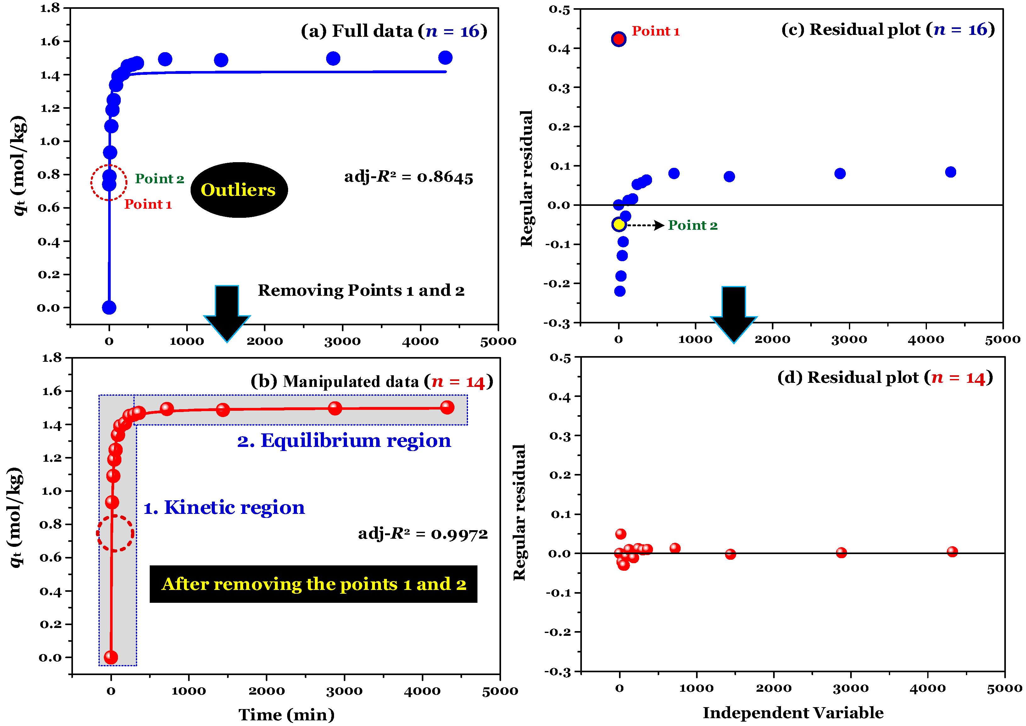
Two regions (kinetic and equilibrium) are observed in Figure 1a. The first region plays an important part in adsorption kinetics because information on the adsorption rate and relevant rate constant is often identified at this region. The second region is plateau points. The PSO and PFO models often tend to fit the adsorption kinetic dataset when the second region (considering specific cases: q_t values are nearly identical at this region) presents in the kinetic curve (the plot of q_t vs. t) [2].

The result of modelling (using the nonlinear method) is shown in Figure 1a. Its adj-R² value was only 0.8645, suggesting that the adsorption process was not well-described by the PSO model. Clearly, the application of the nonlinear method did not provide information as to where the experimental points of time-dependent adsorption are errors.

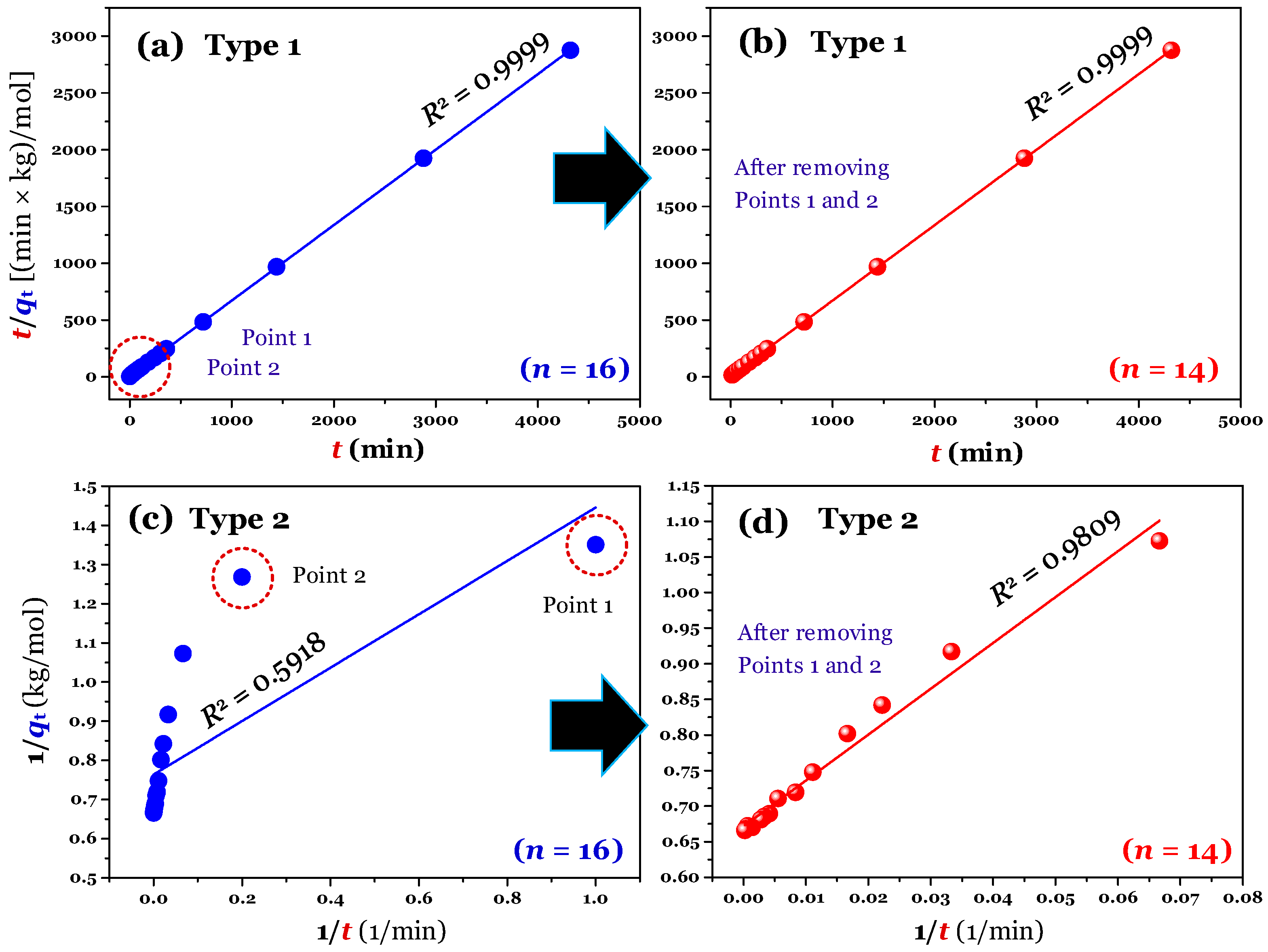
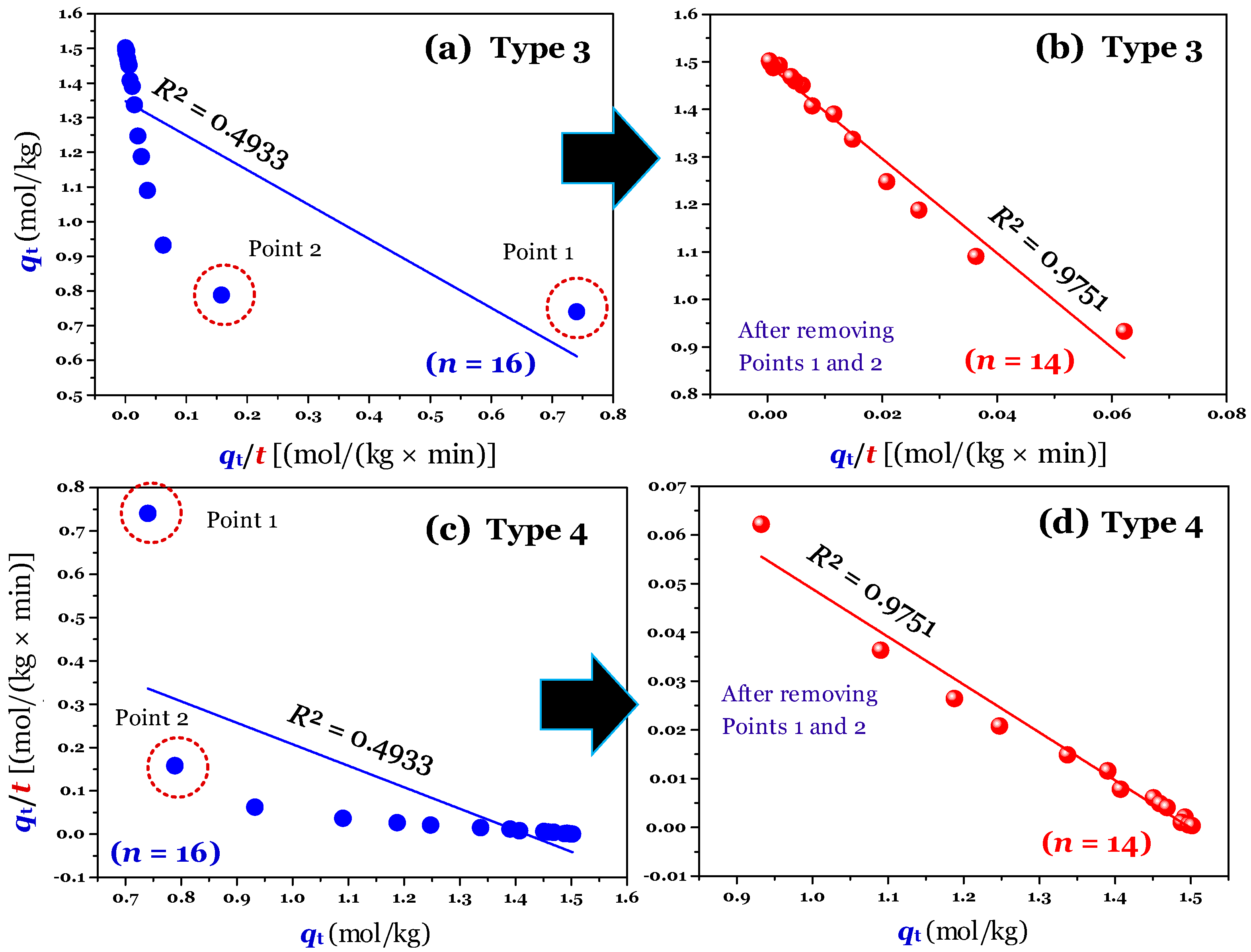
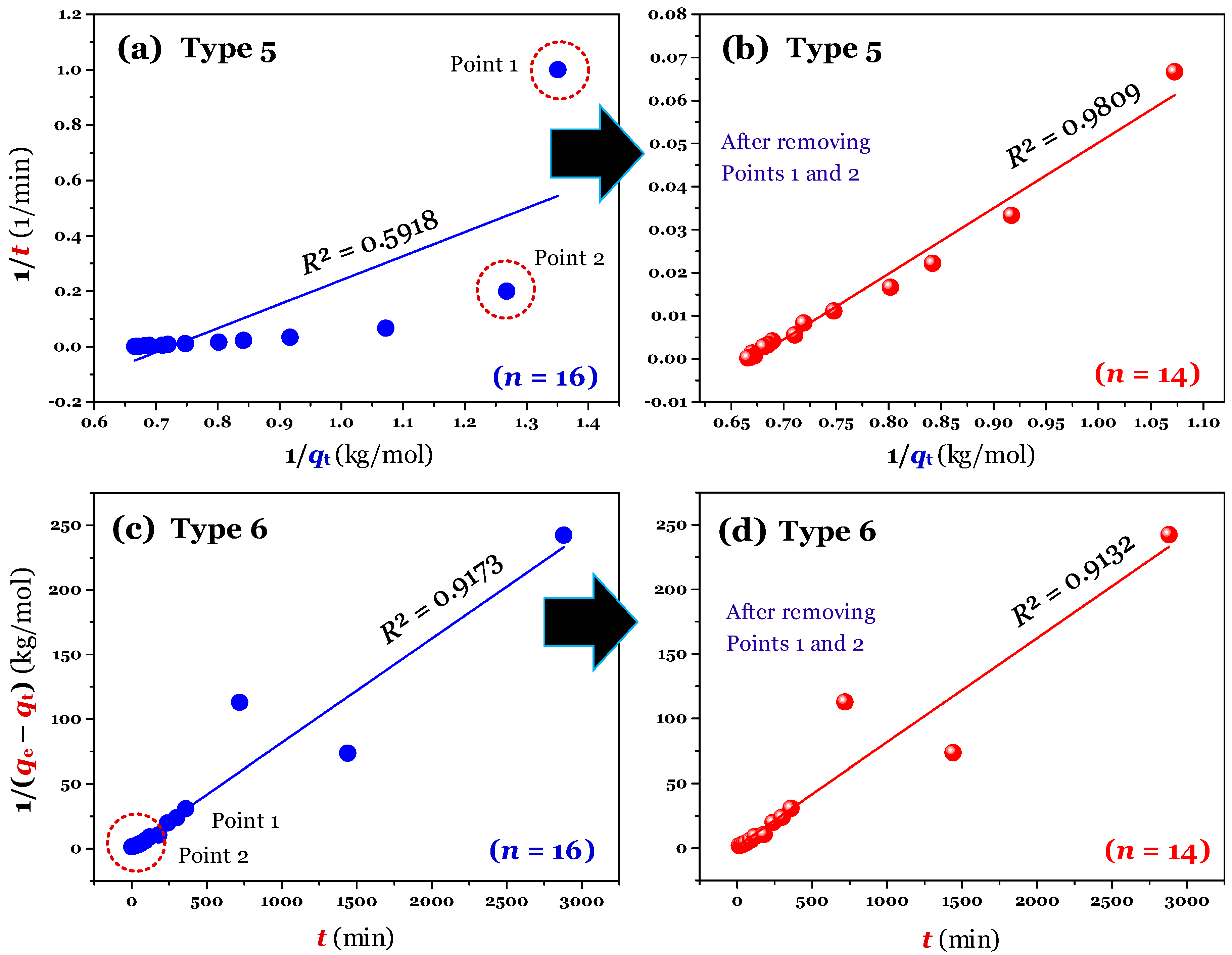
The results (n = 16; full raw experimental data) of modelling (using the linear method) are provided in Figure 2a,c (for Type 1 and 2), Figure 3a,c (for Type 3 and 4), and Figure 4a,c (for Type 5 and 6). Clearly, Type 1 was not helpful for recognizing errors in the experimental points. This is reflected through a very high adj-R² value of 0.9999 (Table 1). A similar conclusion was obtained for Type 6. In contrast, the fault experimental points (denoted as Point 1 and Point 2 in the corresponding figures) were well identified by the others (Types 2, 3, 4, and 5). This is because their R² values only ranged from 0.4571 to 0.5627 (Table 1).

Table 1. Parameters of the pseudo-second-order model obtained from the nonlinear form and its six linear forms.

	Result of Modelling										Result of Re-Modelling
	Full Raw Data (n = 16) *					Manipulated Data (n = 14) **					Revisited Data (n = 16) ***
	k2	qe(2)	adj-R2	χ2	BIC	k2	qe(2)	adj-R2	χ2	BIC	k2	qe(2)	adj-R2	χ2	BIC
1. Nonlinear form
	0.2034	1.419	0.8645	2.2 × 10−2	−61.6	0.0635	1.501	0.9972	4.2 × 10−4	−113.3	0.0635	1.501	0.9985	3.65 × 10−4	−131.0
2. Linear forms
Type 1	0.0711	1.504	0.9999	3.1 × 10−2	−52.1	0.0624	1.504	0.9999	4.6 × 10−4	−104.4	0.0625	1.504	0.9999	4.0 × 10−4	−121.9
Type 2	0.856	1.309	0.5627	3.4 × 10−2	−50.8	0.0701	1.489	0.9793	6.0 × 10−4	−100.8	0.0633	1.504	0.9999	4.0 × 10−4	−121.9
Type 3	0.746	1.348	0.4571	3.1 × 10−2	−52.3	0.0673	1.495	0.9731	6.0 × 10−4	−100.8	0.0641	1.500	0.9953	3.9 × 10−4	−122.1
Type 4	0.3498	1.418	0.4571	2.6 × 10−2	−55.2	0.0656	1.498	0.9731	6.0 × 10−4	−100.8	0.0638	1.501	0.9953	3.9 × 10−4	−122.1
Type 5	0.4543	1.382	0.5627	2.6 × 10−2	−54.8	0.0684	1.492	0.9793	6.0 × 10−4	−100.8	0.0632	1.505	0.9999	4.0 × 10−4	−121.7
Type 6	0.0804	0.703	0.9109	6.3 × 10−1	−3.60	0.0804	0.672	0.9053	6.3 × 10−4	−92.9	0.0805	0.750	0.9173	5.1 × 10−1	−6.938

Notes: * Case 1: results obtained from the raw datasets, ** Case 2: results obtained after removing the outlets (Points 1 and 2; q_t = 0.741 and 0.789 mol/kg); and *** Case 3: results obtained after using the new Points 1 (q_t = 0.131 mol/kg; Table 3) and 2 (0.484 mol/kg; Table 3) estimated from the PSO model (k₂ = 0.0635 and q_e(2) = 1.501); the unit of q_e (mol/kg) and k₂ (kg/(mol × min)); q_e,exp (1.495 ± 0.0061 mol/kg) obtained from the experiment.

Table 1. Parameters of the pseudo-second-order model obtained from the nonlinear form and its six linear forms.

	Result of Modelling										Result of Re-Modelling
	Full Raw Data (n = 16) *					Manipulated Data (n = 14) **					Revisited Data (n = 16) ***
	k2	qe(2)	adj-R2	χ2	BIC	k2	qe(2)	adj-R2	χ2	BIC	k2	qe(2)	adj-R2	χ2	BIC
1. Nonlinear form
	0.2034	1.419	0.8645	2.2 × 10−2	−61.6	0.0635	1.501	0.9972	4.2 × 10−4	−113.3	0.0635	1.501	0.9985	3.65 × 10−4	−131.0
2. Linear forms
Type 1	0.0711	1.504	0.9999	3.1 × 10−2	−52.1	0.0624	1.504	0.9999	4.6 × 10−4	−104.4	0.0625	1.504	0.9999	4.0 × 10−4	−121.9
Type 2	0.856	1.309	0.5627	3.4 × 10−2	−50.8	0.0701	1.489	0.9793	6.0 × 10−4	−100.8	0.0633	1.504	0.9999	4.0 × 10−4	−121.9
Type 3	0.746	1.348	0.4571	3.1 × 10−2	−52.3	0.0673	1.495	0.9731	6.0 × 10−4	−100.8	0.0641	1.500	0.9953	3.9 × 10−4	−122.1
Type 4	0.3498	1.418	0.4571	2.6 × 10−2	−55.2	0.0656	1.498	0.9731	6.0 × 10−4	−100.8	0.0638	1.501	0.9953	3.9 × 10−4	−122.1
Type 5	0.4543	1.382	0.5627	2.6 × 10−2	−54.8	0.0684	1.492	0.9793	6.0 × 10−4	−100.8	0.0632	1.505	0.9999	4.0 × 10−4	−121.7
Type 6	0.0804	0.703	0.9109	6.3 × 10−1	−3.60	0.0804	0.672	0.9053	6.3 × 10−4	−92.9	0.0805	0.750	0.9173	5.1 × 10−1	−6.938

Notes: * Case 1: results obtained from the raw datasets, ** Case 2: results obtained after removing the outlets (Points 1 and 2; q_t = 0.741 and 0.789 mol/kg); and *** Case 3: results obtained after using the new Points 1 (q_t = 0.131 mol/kg; Table 3) and 2 (0.484 mol/kg; Table 3) estimated from the PSO model (k₂ = 0.0635 and q_e(2) = 1.501); the unit of q_e (mol/kg) and k₂ (kg/(mol × min)); q_e,exp (1.495 ± 0.0061 mol/kg) obtained from the experiment.

Table 2. Parameters of some models obtained based on the three cases: full raw data, manipulated data, and revisited data.

	Unit	Result of Modeling (Using the Nonlinear Method)
		Full Raw Data (n = 16) *	Manipulated Data (n = 14) **	Revisited Data (n = 16) ***
qe,exp	mol/kg	~1.495	~1.495	~1.495
1. Pseudo-second-order (PSO) model
qe(2)	mol/kg	1.419	1.501	1.501
k2	kg/(mol × min)	0.2034	0.0635	0.0635
adj-R2	-	0.8645	0.9972	0.9985
red-χ2	-	2.16 × 10−2	4.20 × 10−4	3.65 × 10−4
BIC	-	−61.6	−113.3	−131.1
2. Pseudo-first-order (PFO) model
qe(1)	mol/kg	1.368	1.436	1.428
k1	1/min	0.1792	0.0512	0.0576
adj-R2	-	0.7506	0.9597	0.9710
red-χ2	-	3.98 × 10−2	6.09 × 10−3	6.86 × 10−3
BIC	-	−51.3	−85.6	−81.16
3. Elovich model
α	mol/(kg × min)	126.1	1364	2.913
α	mg/(g × min)	19,073	206,235	440.4
β	kg/mol	9.299	11.11	6.335
adj-R2	-	0.9435	0.9480	0.8700
red-χ2	-	9.03 × 10−3	7.75 × 10−3	3.08 × 10−2
BIC	-	−76.5	−81.5	−55.6
4. Avrami model
qe(AV)	mol/kg	1.536	1.496	1.472
kAV	1/min	0.0973	0.0618	0.0510
nAV	-	0.2913	0.4571	0.6312
adj-R2	-	0.9801	0.9995	0.9935
red-χ2	-	3.17 × 10−3	7.35 × 10−5	1.54 × 10−3
BIC	-	−95.4	−162.1	−107.7
5. Pseudo-nth-order (PNO) model
qe(PNO)	mol/kg	1.933	1.522	1.515
kPNO	kgm−1/(min × molm−1)	0.0268	0.0659	0.0631
m	-	7.299	2.247	2.134
adj-R2	-	0.9605	0.9979	0.9986
red-χ2	-	6.31 × 10−3	3.21 × 10−4	3.25 × 10−4
BIC	-	−83.8	−137.0	−134.1

Notes: * Case 1: results obtained from the raw datasets; ** Case 2: results obtained after removing the outlets (Points 1 and 2; q_t = 0.741 and 0.789 mol/kg) from the raw datasets; and *** Case 3: results obtained after removing Points 1−2 and submitting the new Point 1 (q_t = 0.131 mol/kg; Table 3) and Point 2 (0.484 mol/kg; Table 3) estimated from the PSO model (k₂ = 0.0635 and q_e(2) = 1.501) into the raw datasets.

Table 2. Parameters of some models obtained based on the three cases: full raw data, manipulated data, and revisited data.

	Unit	Result of Modeling (Using the Nonlinear Method)
		Full Raw Data (n = 16) *	Manipulated Data (n = 14) **	Revisited Data (n = 16) ***
qe,exp	mol/kg	~1.495	~1.495	~1.495
1. Pseudo-second-order (PSO) model
qe(2)	mol/kg	1.419	1.501	1.501
k2	kg/(mol × min)	0.2034	0.0635	0.0635
adj-R2	-	0.8645	0.9972	0.9985
red-χ2	-	2.16 × 10−2	4.20 × 10−4	3.65 × 10−4
BIC	-	−61.6	−113.3	−131.1
2. Pseudo-first-order (PFO) model
qe(1)	mol/kg	1.368	1.436	1.428
k1	1/min	0.1792	0.0512	0.0576
adj-R2	-	0.7506	0.9597	0.9710
red-χ2	-	3.98 × 10−2	6.09 × 10−3	6.86 × 10−3
BIC	-	−51.3	−85.6	−81.16
3. Elovich model
α	mol/(kg × min)	126.1	1364	2.913
α	mg/(g × min)	19,073	206,235	440.4
β	kg/mol	9.299	11.11	6.335
adj-R2	-	0.9435	0.9480	0.8700
red-χ2	-	9.03 × 10−3	7.75 × 10−3	3.08 × 10−2
BIC	-	−76.5	−81.5	−55.6
4. Avrami model
qe(AV)	mol/kg	1.536	1.496	1.472
kAV	1/min	0.0973	0.0618	0.0510
nAV	-	0.2913	0.4571	0.6312
adj-R2	-	0.9801	0.9995	0.9935
red-χ2	-	3.17 × 10−3	7.35 × 10−5	1.54 × 10−3
BIC	-	−95.4	−162.1	−107.7
5. Pseudo-nth-order (PNO) model
qe(PNO)	mol/kg	1.933	1.522	1.515
kPNO	kgm−1/(min × molm−1)	0.0268	0.0659	0.0631
m	-	7.299	2.247	2.134
adj-R2	-	0.9605	0.9979	0.9986
red-χ2	-	6.31 × 10−3	3.21 × 10−4	3.25 × 10−4
BIC	-	−83.8	−137.0	−134.1

Notes: * Case 1: results obtained from the raw datasets; ** Case 2: results obtained after removing the outlets (Points 1 and 2; q_t = 0.741 and 0.789 mol/kg) from the raw datasets; and *** Case 3: results obtained after removing Points 1−2 and submitting the new Point 1 (q_t = 0.131 mol/kg; Table 3) and Point 2 (0.484 mol/kg; Table 3) estimated from the PSO model (k₂ = 0.0635 and q_e(2) = 1.501) into the raw datasets.

Table 3. Comparison of the result estimation of some q_t values at the initial periods obtained by different kinetic models and q_t(exp) from the experiment.

Time (min)	qt(exp)	qt Values Estimated Based on the Models					Difference (%) between qt(exp) and qt(model)
		PFO	PSO	PNO	Elovich	Avrami	PFO	PSO	PNO	Elovich	Avrami
1 min (Point 1)	0.741	0.072	0.131	0.151	0.866	0.042	164.7	140.0	132.4	−15.7	178.7
5 min (Point 2)	0.789	0.324	0.484	0.525	1.011	0.197	83.4	47.8	40.2	−24.7	120.0
15	0.933	0.770	0.883	0.905	1.110	0.517	19.1	5.43	3.03	−17.40	57.4
30	1.090	1.127	1.112	1.114	1.173	0.855	−3.290	−1.965	−2.129	−7.258	24.2
45	1.188	1.293	1.217	1.211	1.209	1.076	−8.446	−2.441	−1.928	−1.770	9.846
60	1.247	1.369	1.278	1.268	1.235	1.221	−9.327	−2.389	−1.635	1.005	2.116

Table 3. Comparison of the result estimation of some q_t values at the initial periods obtained by different kinetic models and q_t(exp) from the experiment.

Time (min)	qt(exp)	qt Values Estimated Based on the Models					Difference (%) between qt(exp) and qt(model)
		PFO	PSO	PNO	Elovich	Avrami	PFO	PSO	PNO	Elovich	Avrami
1 min (Point 1)	0.741	0.072	0.131	0.151	0.866	0.042	164.7	140.0	132.4	−15.7	178.7
5 min (Point 2)	0.789	0.324	0.484	0.525	1.011	0.197	83.4	47.8	40.2	−24.7	120.0
15	0.933	0.770	0.883	0.905	1.110	0.517	19.1	5.43	3.03	−17.40	57.4
30	1.090	1.127	1.112	1.114	1.173	0.855	−3.290	−1.965	−2.129	−7.258	24.2
45	1.188	1.293	1.217	1.211	1.209	1.076	−8.446	−2.441	−1.928	−1.770	9.846
60	1.247	1.369	1.278	1.268	1.235	1.221	−9.327	−2.389	−1.635	1.005	2.116

Considering Point 1 and Point 2 in all figures as potential errors, a manipulation was performed by removing Points 1 and 2 from the experimental data. As expected, after manipulating (n = 14), the experimental data of the time-dependent adsorption was adequately described by the PSO model, with the adj-R² values being 0.9972 (for the nonlinear method), and 0.9731−0.9793 (for the linear form of Type 2–5; Table 1). Figure 1b shows that the experimental data (after removing Points 1 and 2 in Figure 1a) were well described by the nonlinear form of the PSO model (adj-R² = 0.9972). Although the evaluation of regular residuals can be used to identify the potential errors within a dataset [11], it is not helpful for many cases. For example, Figure 1c shows that the outlier identification is only visible for Point 1.

Notably, the application of the linear form of Type 1 can lead to misconclusions. This is because its adj-R² values did not change before (adj-R² = 0.9999) and after manipulation (0.9999; Table 1). The difference between the k₂ (0.0711 kg/(mol × min)) value of full data and the k₂ value (0.0624 kg/(mol × min)) of manipulated data obtained from Type 1 was only 13% (Table 1). However, the difference was remarkable for Type 2 (170%), Type 3 (167%), Type 4 (137%), and Type 5 (148%). A similar percentage of the high difference was reported for the case of using the nonlinear method (105%). The result suggested that the use of the linear form (Type 1) of the PSO model can achieve a very high adj-R² value and well describe the experimental data (Figure S1). However, it is very hard to verify whether the parameters of the PSO model are highly believable and accurate. In the literature, some authors have analysed the problems of the linear form of Type 1 [2,21]. They found that although the R² value of Type 1 is very high (even reaching 1), it is a spurious correlation [2,21].

To compare the fitting between the nonlinear and linear methods, the statistical analyses (red-χ² and BIC) were applied. The results (Table 1) demonstrated that the values of red-χ² and BIC obtained from the nonlinear method were lower than those from the linear method. Therefore, the utilization of the nonlinear method can minimize some error functions during the modelling process. A similar conclusion has been reported by some scholars [2,18,19].

It can be concluded that the application of the linear method for calculating the parameters of the PSO model is not highly recommended compared to the nonlinear method. However, the linear method (Type 2, Type 3, Type 4, and Type 5) is very helpful for identifying errors in the experimental points (outliers). The use of Type 1 of the linear form of the PSO model should be undertaken cautiously. This is because it is very hard to identify experimental points and verify the feasibility of the parameters obtained (especially the k₂ value).

4. Other Common Adsorption Kinetic Models

A question is whether other adsorption kinetic models are helpful for identifying errors in the experimental points of time-dependent adsorption. Therefore, it is necessary to use other models for modelling the experimental data. Apart from the PSO model, several models have been used for modelling the time-dependent adsorption data. They include the two- and three-parameter models [8,22,23]. The pseudo-first-order model [24] and Elovich kinetic model [25] are expressed as Equation (14) and Equation (15), respectively [12]. The three-parameter ones are the pseudo-n^th-order model (herein called the PNO model) (Equation (16)) [22,23] (also known as the general-order kinetic model (Equation (17)) [16] and the Avrami-fractional-order model (Equation (18)) [26]. More detailed information on these models has been reported in some documents [16].

$$q_{\mathrm{t}}=q_{\mathrm{e}(1)}\left[1-\exp (-k_{1}t)\right]$$

(14)

$$q_{\mathrm{t}}=\frac{1}{\beta }\mathrm{l}\mathrm{n}(1+\alpha \beta t)$$

(15)

$$q_{\mathrm{t}}=q_{\mathrm{e}(\mathrm{PNO})}-\frac{q_{\mathrm{e}(\mathrm{PNO})}}{{\left[1+\left(\mathrm{m}-1\right)q_{\mathrm{e}(\mathrm{PNO})}^{\left(m-1\right)}{\mathrm{k}}_{\mathrm{P}\mathrm{N}\mathrm{O}}t\right]}^{\frac{1}{m-1}}}$$

(16)

$$q_{\mathrm{t}}=q_{\mathrm{e}(\mathrm{PNO})}\left\{1-{\left[\frac{1}{1+\left(\mathrm{m}-1\right)q_{\mathrm{e}(\mathrm{PNO})}^{\left(\mathrm{m}-1\right)}{k}_{\mathrm{PNO}}t}\right]}^{\frac{1}{m-1}}\right\}$$

(17)

$$q_{\mathrm{t}}=q_{\mathrm{e}(\mathrm{A}\mathrm{V})}\left[1-{\exp (-k_{\mathrm{A}\mathrm{V}}t)}^{n_{\mathrm{A}\mathrm{V}}}\right]$$

(18)

where q_t (mol/kg) is defined in Equation (2); k₁ (1/min), k_PNO (kg^m−1/(min × mol^m−1)), and k_AV (1/min) are the adsorption rate constants of the PFO, PNO, and Avrami models, respectively; q_e(1), q_e(PNO), and q_e(AV) are the adsorption capacities of CAC towards paracetamol at equilibrium (mol/kg) estimated by the PFO, PNO, and Avrami models, respectively; m and n_AV are the exponents of the PNO and Avrami models; α (mol/(kg × min)) and β (kg/mol) are the initial rate and the desorption constant, respectively, of the adsorption kinetics of the Elovich model.

In general, the PFO and PSO models are frequently used in the literature. Unlike the PSO model, the linear form of the PFO model (Equation (19) or Equation (20)) indicates two unknown parameters that are q_e(1) and k₁. The parameter q_e(1) must be selected before applying the linear method. However, it is not easy to select q_e(1) appropriately. If q_e(1) is lower than (or equal to) q_t, the result of calculating ln(q_e(1) − q_t) is an error (#NUM!). By selecting q_e(1) slightly higher than the highest value of q_t, the result of fitting the linear method is provided in Figure S2. Clearly, the errors in the experimental datasets of time-dependent adsorption (i.e., Points 1 and 2) were not detected through the linear fitting of the PFO model (Figure S2).

$$\ln (q_{\mathrm{e}(1)}-q_{\mathrm{t}})=-k_{1}t+\ln (q_{\mathrm{e}(1)})$$

(19)

$$\log (q_{\mathrm{e}(1)}-q_{\mathrm{t}})=-\frac{k_1}{2.303}t+\log (q_{\mathrm{e}(1)})$$

(20)

For the three-parameter models, the application of the linear method for computing the parameters is not suitable. Therefore, the nonlinear optimization method is applied for calculating the parameters of those kinetic models using full data (n = 16; Figure 1a) and manipulated data (n = 14; Figure 1b). Furthermore, to obtain a fair comparison between the two- and three-parameter models, the BIC statistics were used to assess the best-fitting model [2].

The result of modelling is provided in Figure S3 and Table 2. For the full data (n = 16), the fitting model followed the order of the Avrami model (BIC = −95.4) > PNO model (−83.8) > Elovich model (−76.5) > PSO (−61.6) > PFO (−51.3). Notably, some models indicated a doubtful result. For example, the m of the PNO was 7.299; this means that the overall order of the adsorption process was up to seven (an impossible result for the adsorption kinetics). However, the results (Figure S3 and Table 2) do not indicate which of the experimental points of the time-dependent adsorption are errors. The conclusion is consistent with the previous finding in Section 2.

Furthermore, Points 1 and 2 in Figure 1a are assumed to be outliers (errors). After removing them from the raw data, the result of modelling (based on Figure 1b; n = 14) indicates that the best-fitting models were in the following order: the Avrami model (BIC = −162.1) > PNO model (−137.0) > PSO model (−113.3) > PFO model (−85.6) > Elovich model (−81.5). The three-parameter models (i.e., the Avrami and PNO models) indicated the best description for the current experimental data compared to the two-parameter ones. The overall order of the adsorption kinetics (obtained based on the PNO model; m = 2.247) was close to two (feasibly considering it as the PSO model).

5. Re-Modelling Using Points 1 and 2 Estimated from the PSO Model

After removing the two outliers, the results of modelling (n = 14) are listed in Table 2. Using the parameters of the models, the values q_t at 1 min (Point 1) and 5 min (Point 2) are estimated. The results (Table 3) indicated a remarkable difference between the q_t value obtained from the experiment (q_t(exp)) and the q_t value estimated from the model (q_t(model)). Taking the case of the PSO model as a typical example, the values q_t(exp) at 1 min and 5 min (0.741 and 0.789 mol/kg) are overwhelming higher than those obtained from the PSO model (0.131 and 0.484 mol/kg, respectively). The differences between q_t(exp) and q_t(model) are 140% for Point 1 and 47.8% for Point 2 (Table 3). The result confirms again that they (Points 1 and 2) were errors and outliers.

The q_t values for Point 1 (0.131 mol/kg) and Point 2 (0.484 mol/kg) are estimated by the PSO model. After submitting these estimated points into the datasets, the results of re-modelling are provided in Figure S4 and Table 2 (revisited data). The fitting model followed the decreasing order: the PNO model (BIC = −134.1) > PSO model (−131.1) > Avrami model (−107.7) > PFO model (−81.16) > Elovich model (−55.6). The results indicate that the Elovich and Avrami models can be considered empirical equations used for physically fitting the experiential data of time-dependent adsorption. In particular, the initial rate α of the Elovich model (Table 2) indicated a remarkable change of 19,073 mg/(g × min) for the full raw data (n = 16), 206,235 mg/(g × min) for the manipulated data (n = 14), and 440.4 mg/(g × min) for the manipulated data (n = 16). The exponent n_AV of the Avrami model that does not provide information on the overall order of the adsorption process only serves an empirically adjusted parameter. Unlike those models, the PNO model (especially its exponent m) is helpful for initially checking whether the datasets are feasible or not. The overall order of the adsorption process (m) was 2.134, which is close to the second order.

Because the linear forms of the PSO model are helpful for identifying the outlets from the initial period of the databases, it is necessary to re-verify this conclusion. After submitting the two estimated points into (Point 1 (q_t = 0.131 mol/kg) and Point 2 (0.484 mol/kg)) the datasets, the results of re-modelling using six linear forms of the PSO model are provided in Figure S5 and Table 1. As expected, the errors (Points 1 and 2) in the experimental datasets are not observed in Types 1–5, suggesting that the application of the linear form (i.e., Types 1–5) of the PSO model can help to identify these potential errors in the initial adsorption period.

In contrast, Type 1 of the PSO model fitted the experimental datasets well (adj-R² = 0.9999) when considering three cases: the full raw data (n = 16), manipulated data (n = 14), and manipulated data (n = 16) in Table 1; therefore, it is impossible to verify whether there are errors in the datasets or not. Type 6 should not be used because it must first estimate the unknown q_e value as in the case of the linear form of the PFO model. 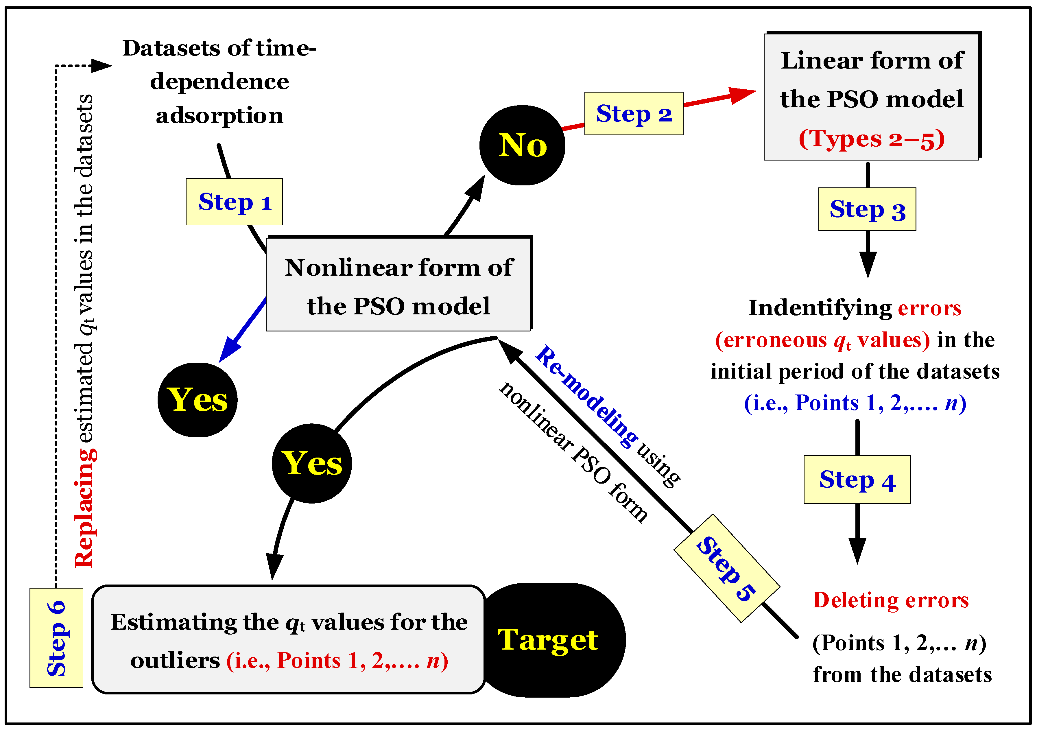Figure 5 provides a brief summary of the validation and re-verification processes of the time-dependent adsorption data. Adsorption kinetic curves (q_t vs. t) must indicate an equilibrium region (as showed in Figure 5).

Notably, the conclusions of this work might be feasible for some normal adsorption processes. Although other contributions (n−π interaction, hydrogen bonding formation, and π−π interaction) existed in the adsorption process of organic pollutants (i.e., PRC), pore filling has been identified as a primary mechanism of PRC into CAC [27] and other porous carbonaceous materials (such as spherical and nonspherical biochars [28]). Those mechanisms were acknowledged as physical adsorption because of low magnitudes of standard adsorption enthalpy change (ΔH° = 6.36–24.1 kJ/mol) [27,28]. Therefore, the process for the validation and re-verification of the time-dependent adsorption data (Figure 5) needs to be applied.

In contrast, the adsorption process of heavy metals (i.e., Cd) onto some CaCO₃-enriched materials occurred very fast at the first period of adsorption. The primary adsorption was surface precipitation such as Cd(CO₃) and/or (Cd,Ca)CO₃ [5,29]. This mechanism was known as nonactivated chemisorption that often occurs very rapidly and has low activation energy [29,30]. It might not be necessary to recheck the initial periods of the time-dependent adsorption datasets. This is because it is the nature of nonactivated chemisorption [3,30].

6. Conclusions

Applying the nonlinear optimization method for modelling the time-dependent experimental data is recommended. However, this nonlinear method does not provide relevant information on errors in the experimental points (potential outliers). This method should only be applied after the outliers are identified and removed. Results showed that the utilization of the linear forms (Types 2–5) of the PSO model was appropriate for identifying errors in the experimental points (at the initial adsorption period) of time-dependent adsorption. This conclusion is valid when the plot of q_t vs. t indicates two regions: kinetics and equilibrium (equilibrium is a plateau region).

Type 1 was physically well-fitted to the full raw experimental data, manipulated data (adj-R² = 0.9999; n = 14), and revisited data (adj-R² = 0.9999; n = 16). However, it (adj-R² or r²) has been denoted as a spurious correlation in some cases. The application of Type 1 for calculating the parameters (q_e(2) and k₂) should be avoided because it is hard to validate the accuracy of these parameters. For Type 6, the q_e value must be firstly estimated (a similar case of the linear form of the PFO model); therefore, its parameters obtained did not bring a high accuracy.

The PNO model can give some general information on doubts in the datasets. For example, its exponent m (7.299) is very high when considering the full raw data but suitable when considering the manipulated data (m = 2.247) and the revisited data (m = 2.134 that can be called the overall order of the adsorption process). However, this model did not provide where the outlets are located in the datasets.