Article

Estimating Land Subsidence and Gravimetric Anomaly Induced by Aquifer Overexploitation in the Chandigarh Tri-City Region, India by Coupling Remote Sensing with a Deep Learning Neural Network Model

by
Arjuman Rafiq Reshi
1,
Har Amrit Singh Sandhu
1,
Claudia Cherubini
2 and
Akshar Tripathi
3,*
1
Department of Civil Engineering, Punjab Engineering College (PEC), Chandigarh 160012, India
2
Department of Environment and Prevention Sciences, University of Ferrara, 44121 Ferrara, Italy
3
Department of Civil & Environmental Engineering, Indian Institute of Technology (IIT) Patna, Bihar 801106, India
*
Author to whom correspondence should be addressed.
Water 2023, 15(6), 1206; https://doi.org/10.3390/w15061206
Submission received: 20 February 2023 / Revised: 10 March 2023 / Accepted: 17 March 2023 / Published: 20 March 2023
(This article belongs to the Special Issue Groundwater Management in a Changing World: Challenges and Endeavors)

Abstract

:
This study utilizes surface displacement data from Persistent Scatterer SAR Interferometry (PSInSAR) of Sentinel-1 satellite and groundwater storage change data from the Gravity Recovery and Climate Experiment (GRACE) satellite mission to understand land subsidence in the Chandigarh tri-city region. The satellite datasets are used along with the groundwater level data obtained from wells over the study area. Since the GRACE data are available at a much coarser spatial resolution of 1o by 1o, challenges remain in correlating the dataset with PSInSAR displacement that has been multi-looked at 14 m by 14 m resolution. Therefore, multiple sources of data (i.e., the monthly average of GRACE data, groundwater storage change and monthly average PSInSAR displacement per pixel, and interpolated groundwater level data from wells for 2017 to 2022) have been deployed into a deep learning multi-layer perceptron (DLMLP) model to estimate the groundwater storage change at the urban level. This has an indirect downscaling method that is carried out successfully using the DLMLP model for the estimation of groundwater storage changes at the urban level, which is usually complicated by applying direct downscaling methods on the GRACE data. Thus, the DLMLP model developed here is a distinctive approach considered for estimating the changes in groundwater storage using PSInSAR displacement, groundwater data from wells, and GRACE data. The DLMLP model gives an R2-statistics value of 0.91 and 0.89 in the training and testing phases, respectively, and has a mean absolute error (MAE) of 1.23 and root mean square error (RMSE) of 0.87.

1. Introduction

With the induction of machine learning in the field of remote sensing, it has now been possible to make estimations of several Earth observation phenomena with high accuracy [1]. Groundwater is an important resource, and its depletion is causing surface displacement across many regions of India [2]. The application of machine learning algorithms such as deep learning neural networks can help to make an accurate estimation of surface displacement and groundwater storage [3].
The urban environment has been the cradle of industrial advancement, institutional functioning, and government functionality [4]. With the increasing human population and the drastic changes in land use/land cover, regular monitoring of the resources and the urban environments becomes necessary [5].
The unregulated and unplanned groundwater extraction is causing a heavy stress on groundwater resources [6]. The groundwater reserves are drying up faster than they can be recharged by the rainfall. This is resulting in a net deficit in underground hydrostatic pressure and urban surface subsidence [7]. The problem is equally evident in non-riverine towns as well as cities located on riverbanks where the river water supply systems are not sufficient to cater to the needs of a huge population. For cities located on the foothills of the Himalayas, that lie in seismic zones IV and V, such surface subsidence is not a good sign. Any seismic activity or earthquake can cause a serious disaster with an already subsiding ground surface [8]. To map the surface displacements, time series remotely sensed data today have been successfully applied in different studies all over the world [9,10].
India is blessed with some of the mightiest river systems in the world and many big cities developed on their banks [11]. The water from rivers and lakes near a city is the major and most obvious source of a potable water supply. However, with the exponential population increase, the civic water supply infrastructure is often not sufficient to cater to the needs of everyone. The problem becomes more severe for cities such as Chandigarh that are located far from any perennial source of water and depend only upon the groundwater to meet their water requirements. Groundwater overexploitation together with a deficit in rainfall cause depletion of the groundwater storage [12,13]. Over the years, the land surface subsidence becomes too severe to handle and leads to the need for an urgent evacuation and relocation of the entire urban population and infrastructure, as in the case of megacities such as Jakarta (Indonesia) [14,15].
Persistent Scatterer SAR Interferometry (PSInSAR) is another emerging field of research in the arena of SAR remote sensing [16]. Several studies have applied SAR interferometry techniques to monitor land subsidence [17]. They have found successful applications to study seismic and geological effects using a technique widely known as Differential SAR Interferometry (DInSAR), wherein the same sensor flies successively over the same location with the same geometry [18]. Any movement of the ground feature temporally is caught by correlating it with the phase difference in the incoming RADAR backscatter in DInSAR [19]. Similarly, SAR remote sensing is being used with various machine learning models for a variety of applications such as the PSInSAR-based urban surface subsidence estimation [20]. The PSInSAR is a form of Differential SAR Interferometry where the built-up features that act as permanent or persistent scatterers are taken as reference features, and the line of sight (LOS) displacements are studied concerning these permanent scatterers [21,22].
Zhang et al. (2011) [23], applied the interferometric point target analysis (IPTA) technique for mapping the ground subsidence in Suzhou city, Jiangsu province, China. They analyzed thirty-four ERS-1/2 SAR scenes and produced the deformation information of over 38,881 point targets between 1992 and 2000. The results showed that the IPTA-derived deformation estimates corresponded well with levelling measurements.
Ng et al. (2017) [24] compared the simulation and real data analysis results from the recently launched SAR satellites, ALOS-2, Sentinel-1, and Radarsat-2, for monitoring subsidence induced by longwall mining activity using satellite synthetic aperture radar interferometry (InSAR). Their results showed that the three satellites performed better than their predecessors. The simulation results showed that the Sentinel-1A/B satellites were capable of mapping rapid mine subsidence, especially the Sentinel-1A/B with stripmap (SM) mode.
Liosis et al. (2018) [25] applied SAR interferometry to monitor ground subsidence in the rural area of Al Wagan, UAE. The results revealed a localized subsidence phenomenon which was speculated to be groundwater related. It was observed from different sensors that subsidence velocities reached 18 cm/year during 2003–2010 with the cumulative displacements exceeding −1 m. However, it appeared to be slightly more stable during the more recent past (December 2016–March 2018) as observed in the results with recent Sentinel-1 data where a maximum localized subsidence in the order of 10 cm was estimated.
Chen et al. (2019) [26] applied a small baseline InSAR technique to process Envisat ASAR images acquired between 2003 and 2010 and TerraSAR-X stripmap images collected from 2010 to 2011 to investigate land subsidence in the Beijing region. A high correlation was observed between InSAR subsidence rate maps derived from two different datasets (i.e., Envisat and TerraSAR-X). They concluded that InSAR was a powerful tool for monitoring land subsidence.
In the recent past, among the few notable studies conducted in India on SAR interferometry, the study conducted by Tiwari et al. (2020) [27] is important since it utilized LiDAR and GNSS datasets along with SAR data for landslide-induced surface displacement. The study successfully mapped a mean displacement velocity in the range of −0.110 to 0.008 mm/year and gave good evidence of sensor interoperability between LiDAR and Sentinel-1 SAR.
In the study conducted by Monika et al. (2022) [28], the PSInSAR technique was applied for the estimation of land surface displacement due to the underground mining of the Korba region of Chattisgarh in India. The study utilized Sentinel-1 SAR data and ground measurements for the mapping of surface subsidence between 2015 and 2017 and estimated it to be 3–21 mm/year along the line of the prospect of the SAR sensor.
The study conducted by Awasthi et al. (2022) [29] is one of the few bold attempts that have rightly proved that urban surface subsidence is due to groundwater exploitation. The study utilized optical multi-spectral data from Landsat-5 and 8 for the analysis of urban land use growth patterns apart from GRACE data and groundwater well data for correlating the findings of PSInSAR-based urban surface subsidence.
The urban built-up is a permanent land use feature and acts as a persistent (permanent) scatterer for incident Synthetic Aperture RADAR (SAR) signals from an active SAR satellite sensor [30]. This study utilized C-band Single Look Complex (SLC) datasets from Sentinel-1 satellite for Persistent Scatterer SAR (PSInSAR)-based urban surface subsidence estimation and mapping. This study also utilized groundwater storage change data from the Gravity Recovery and Climate Experiment (GRACE) satellite, along with the groundwater level data from the Chandigarh tri-city region for an analysis of groundwater level fluctuations. Since the GRACE data are available at a resolution of 1o × 1o and downscaling them to the city level is very difficult, the observations were used to develop a deep learning neural network model that gave the per pixel groundwater storage change for Chandigarh tri-city based on the per pixel urban surface subsidence at 14 m by 14 m spatial resolution. Such studies are important since downscaling certain datasets such as GRACE is not possible beyond a certain dimension without the loss of information.
Most of the studies conducted for PSInSAR-based urban surface subsidence and GRACE data have mentioned groundwater exploitation as one of the root causes of land subsidence. However, all these studies have been supplemented by data from wells in their respective study regions. The challenge is obvious, as none of the studies has been able to downscale or suggest a novel method of downscaling the GRACE data from 300 km by 300 km spatial resolution to the city level. This study made a novel approach by exploring the interoperability of Sentinel-1 SAR and GRACE satellite sensors for a PSInSAR-based urban surface subsidence analysis. This study also used the PSInSAR-based surface subsidence values, GRACE data, Global Land Data Assimilation System (GLDAS) Land Surface Model (LSM), and groundwater data from wells in Chandigarh tri-city region for the estimation of groundwater storage change values at the city level using a deep learning multi-layer perceptron model, which is largely missed by the contemporary studies.
The objectives of the study are-
  • Use freely available C-band Sentinel-1 SAR data-based PSInSAR for urban surface displacement mapping of Chandigarh tri-city region from 2017 to 2022, thus making the study cost-effective.
  • Explore the interoperability of C-band SAR and GRACE gravimetric satellite sensors for groundwater exploitation-induced groundwater storage change.
  • Estimate the groundwater storage at the city level using the DLMLP model and PSInSAR, groundwater data from wells, and GRACE data as parameters.

2. Materials and Methods

2.1. Study Area

The study area is India’s first planned township of the Chandigarh tri-city region, which also serves as the joint capital of Punjab and Haryana states in India [31]. Apart from the remotely sensed Sentinel-1 SAR and GRACE satellite datasets, groundwater level data have also been used for this study.
The region is located on the foothills of the Shivalik mountains and covers an area of 114 km2 between 30.74° N and 76.79° E. The region enjoys a monsoon type of climate with hot summers from April to June, monsoons from July to September, and winters from October to March. Being the first planned city of independent India, the city of Chandigarh is based on the iron grid pattern with streets crossing at 90-degree angles.
Due to administrative reasons, Chandigarh was renamed as the Chandigarh capital region or Chandigarh tri-city that today comprises the Union Territory of Chandigarh, Mohali, Kharar, Zirakpur, New Chandigarh (in Punjab), and Panchkula (in Haryana) [32]. A detailed study area map is shown in Figure 1.

2.2. Hydro Geology of Chandigarh Tri-City Region

Semi-consolidated formations from the middle Miocene age of the upper Shiwalik system occupy the Chandigarh region [33]. These formations are mostly exposed in the northeast while the rest of the area is occupied by the Pleistocene age Indo Gangetic alluvium [34]. The formations are a result of the deposition carried out by the drainage system that originates in the Shiwalik in the northwest and southeast of Chandigarh [35]. There is a sharp contrast as coarser sediments occur along the southeastern region while finer sediments occur along the northwestern region, and this restricts the aquifer disposition laterally. The coarser boulder-gravel-sand depositions are not prevalent in the area since the source formations are mostly fine-grained. Based on the excavations carried out by the Central Ground Water Board (CGWB), it has been observed that the region has fair-to-good aquifer horizons, except in the southwest (http://cgwb.gov.in/District_Profile/Chandigarh/CHANDIGARH.pdf, accessed on 15 September 2022).
At some places, however, it is also inferred that up to 180 m below ground level (180 mbgl), the sediments are coarse-grained and become finer at depths more than 180 m [36]. This is evidence of a good aquifer recharge potential of the region during rainfall. The CGWB carried out several explorations to determine the groundwater levels and the structure of aquifers in the Chandigarh region [37]. It has been observed that a 20 m thick confined aquifer exists all around the Chandigarh region at 160 mbgl, except sector 38 which has the presence of medium-to-coarse sand [38]. From the explorations, it was also inferred that the yield of the deeper aquifers at more than 180 mbgl is also less as compared to the shallow ones at less than 180 mbgl. The groundwater in the Chandigarh region occurs under the water table in confined as well as semi-confined states. The pumping tests conducted by the CGWB also revealed that there are good, confined aquifers occurring in sectors 33, 10, and 47, while there are leaky aquifers encountered around sector 28. The CGWB report for 2021 gives a detailed account of the aquifers in the Chandigarh region- http://cgwb.gov.in/GW-Assessment/GWR-2020-Reports%20State/2022-03-14_GWRE%20Report%202020%20Chandigarh.pdf, accessed on 15 September 2022.

2.3. Materials

The details of the datasets used for this study are mentioned in Table 1.
As shown in Table 1, for this study, the Single Look Complex (SLC) Synthetic Aperture RADAR (SAR) data from the Sentinel-1 satellite, groundwater level data from the Central Ground Water Board (CGWB), Gravity Recovery and Climate Experiment (GRACE) satellite data on a monthly basis, and Global Land Data Assimilation System—Land Surface Model (GLDAS-LSM) soil moisture and surface water storage data from NASA were used.

2.4. Methods

Dual Polarized (VV + VH polarization channel) time series Sentinel-1 SAR Single Look Complex (SLC) datasets were used for this study. The SLC datasets were acquired in Interferometric Wide (IW) swath mode and were subsets to isolate the study area from the relevant IW sub-swath. This was followed by pre-processing, where the Sentinel-1 SAR data were split to delineate the IW sub-swath image tile with the study area. The split imagery was deburst since the imagery was acquired in burst SAR mode. After that, the digital number (DN) values of pixels were correlated with the SAR backscatter using the calibrate operation (further details in Section 2.4.1). The pre-processed datasets were then co-registered with respect to the image from 2017 which was taken as the master image, and the subsequent imageries were stacked as slave images. A total of 70 images (35 in ascending and 35 in descending passes) were co-registered together in the VV and VH polarization channels. The co-registered stack was then multiplied by the complex conjugate of itself for the generation of an interferogram. Since the phase angle of the interferogram swapped to 0, every time it encountered a 2π phase cycle, the phase was unwrapped for better image interpretation and analysis. This unwrapped phase was then used for the calculation of line of sight (LOS) displacement which is indicative of surface subsidence. After the calculation of the surface subsidence, it was important to perform a time series analysis to ascertain the displacement of permanent scatterers over time. For the time series analysis, it was necessary to remove the atmospheric phase screen (APS), since the APS causes errors in the SAR signals in the LOS making the time series analysis difficult [39]. After the APS removal, the persistent scatterer (PS) points were selected throughout the study area using a coherence threshold of 0.3. Based on the 7519 PS identified, any random point was selected for the time series analysis since the PS was stationary concerning the built-up feature it was located upon, but not with respect to the ground. This makes the study of any movement such as the cumulative LOS displacement, height, and velocity, easier, over a period.
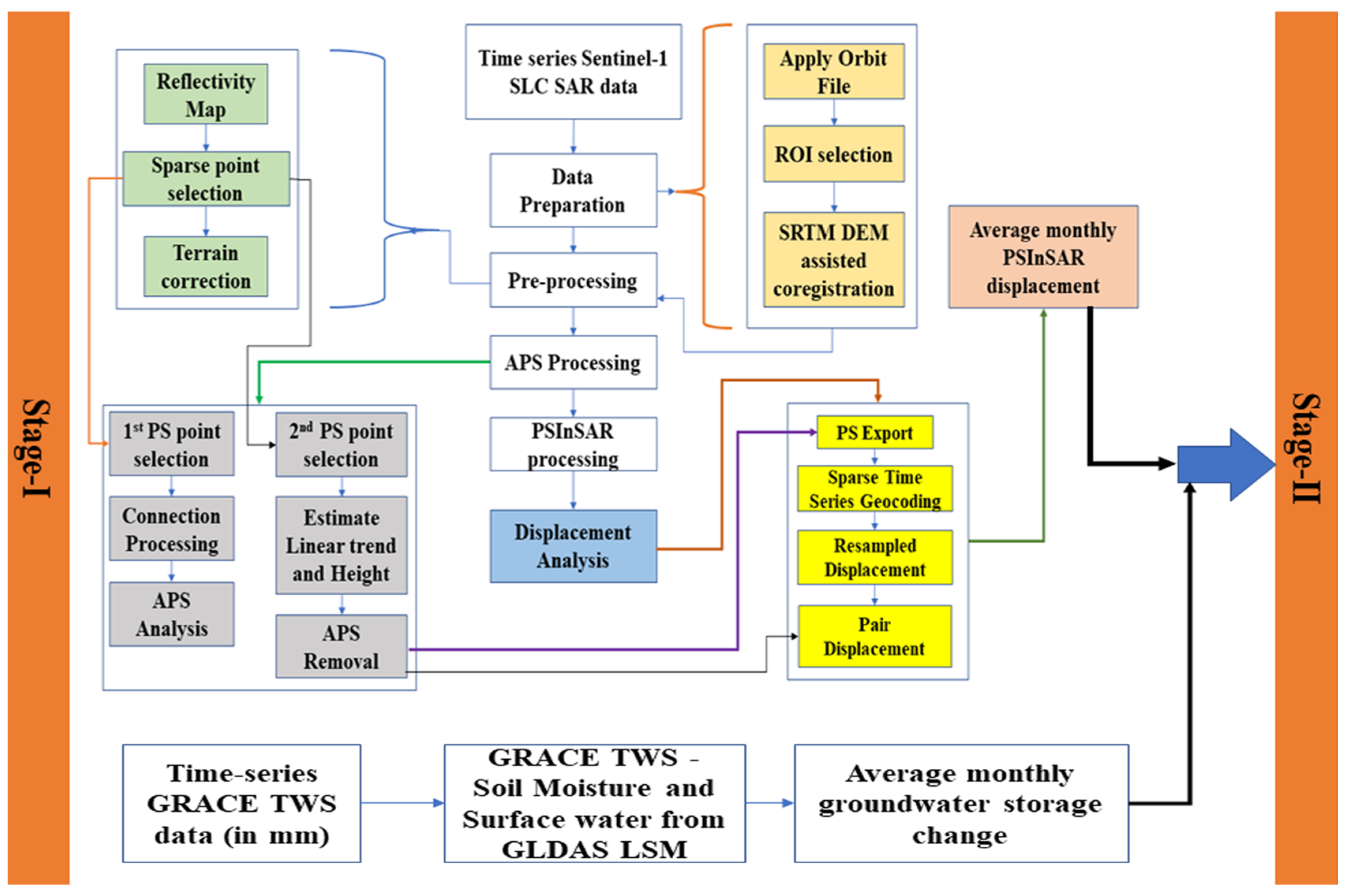
The GRACE data were correlated with the monthly average PSInSAR surface subsidence findings. After that, the surface subsidence data from Sentinel-1 PSInSAR, and gravimetric data from GRACE were fed into a deep learning multi-layer perceptron model, and an estimation was carried out for the per pixel groundwater storage change (ΔGWS) in the entire study area. The estimated ΔGWS was correlated with the groundwater level data from borewells at 25 locations in the study area. The detailed methodology flow diagram is shown in Figure 2.

2.4.1. SAR Data Pre-Processing

Every SLC image of Sentinel-1 is made up of three sub-swaths or IW products [40]. It is important to isolate the IW sub-swath containing the study area from the SLC product [41]. The process was termed the Sentinel-1 Terrain Observation with Progressive Scans (TOPS) split. After that, the Sentinel-1 image containing the precise study area was calibrated to remove any radiometric errors in the imagery and to relate the digital number (DN) values of the image to the SAR backscatter from the target, using the following equation [42].
value ( i ) = D N i 2 A i 2
where value (i) is the original DN value, and Ai is the backscatter coefficient denoted as sigma nought (σ0). After that, since the SAR images are acquired in burst mode or beam mode, to further radiometrically correct the SAR imagery, it is deburst [43]. The deburst operation is followed by the multi-look operation where square pixels are generated from the SAR image having different spatial resolutions in range and azimuth directions (5 m × 20 m to 14 m × 14 m). The multi-look is carried out in the spatial domain using a 2D convolution as well as in the frequency domain using the spectral mixing method [44]. For this study, the multi-look was carried out in the spatial domain.
After that, the multi-looked imagery was further orthorectified using a terrain correction operation where the image coordinates were related to the actual ground coordinates using a Shuttle RADAR Topography Mission (SRTM) plugin.

2.4.2. SAR Data Interferometric Processing

After pre-processing, all 52 images both in the ascending and descending passes were co-registered into a single co-registered stack. In co-registration, all images are arranged and aligned with respect to one master image. This is done to align the image features with respect to one image (master image) so that any topographical changes that occur in the subsequent images (slave images) are captured easily [45]. This is helpful when studying the LOS displacements and performing a time series analysis. After the co-registration process, coherence was estimated, which is a measure of the permanence of features and its value varies between 0 to 1. The coherence image helps to identify the persistent scatterers having values close to 1. The coherence estimation was carried out by the following equation [46].
γ = E [ i m g   i . i m g   k ] E i m g   k . 2 E . [ i m g   i ] 2
where γ represents the assemblage averaging function of the sample data, and imgi and imgk represent the master and slave images, respectively. After that, an interferogram was generated for image pairs from 2017–18, 2018–19, 2019–20, 2020–21, 2021–22, and finally for 2017–22-time frames. The interferogram was generated by multiplying the co-registered stack with the complex conjugate of itself using the following equations [47,48].
ɸ 1 = 4 π λ
ϕ 2 = R + Δ R / λ
ϕ2 − ϕ1 = 4π (ΔR)/λ
where R is the target distance and Φ is the phase information. A proper interference is needed between the master and the subsequent slave imageries so that the PS features maintain sufficient coherence for the interferometric analysis. Finally, after the phase was unwrapped from the interferogram, the unwrapped phase was used for the estimation of LOS displacement as shown by Equation (6) [49,50].
Surface   Displacement = ( ϕ   u n w . p h a s e ) λ / 4 π . c o s θ
where λ is the wavelength and θ is the angle of incidence.

2.4.3. Atmospheric Phase Screen (APS) Removal

The time series SAR datasets face temporal and geometric signal decorrelations mainly due to the tropospheric turbulence and stratifications [51]. To remove the signal attenuation effects on the SAR signals, it is important to correct the distortions in the SAR imagery that arise out of atmospheric effects. The process of atmospheric distortion removal in SAR images is termed APS removal. Today, there are many algorithms to carry out APS removal; however, the statistical convolution technique is generally followed, as has been used in this study.

2.4.4. Time Series Analysis

As was explained in the methodology section, coherence was used as an indicator for the permanence of the features under study; therefore, for the time series analysis, the persistent scatterer points must be selected with ultimate precision. Since in each area of Chandigarh, there are numerous persistent scatterer points, and the study of each one of these is difficult, a few points were selected for the stability studies over the selected period. The logic behind the selection of a stable point is that the higher the backscatter energy received at the sensor, the higher the stability of the selected PS point. Therefore, the point with the highest backscatter energy was selected first automatically by the SARPROZ among a cluster of PS points, and then a manual user-based selection of PS points was made based on the area of particular interest of the user [52]. These PS points were named as 1st (automatically selected) and 2nd (manually selected) PS points, respectively. After that, a 5 mm/year linear parameter for every 20 m height change was selected as the default for studying the LOS displacement that occurred over time between the set of images used. The selection of the values was made after a careful literature survey which revealed that most of the studies have used this as a standard for the time series PSInSAR analysis for displacement velocity in mm/year to residual height variations. After the removal of the APS, a coherence connection graph was obtained for the PS points selected as shown in Figure 3.

2.4.5. GRACE Data Processing

Any change in the mass of the Earth causes a change in gravimetry as well [53]. Of the different factors contributing to the mass of the Earth or its gravimetry, the groundwater reserves are the most dynamic [54]. This groundwater is stored in the sub-surface strata and any variation in the levels is reflected in the gravimetric values as well [55]. These gravimetric fluctuations were recorded in the 1° × 1° spatial resolution data of the GRACE satellite sensor [56]. The data from GRACE are available in. netCDF and .tif for-mats and were orthorectified using the SRTM plugin for terrain correction [57]. Thereafter, the study area was clipped using the boundary shape file of the study area. The GRACE data was used at every 12 days repeat passes, as the Sentrinel-1 SAR data. Since the GRACE data had a very coarse spatial resolution, only the average ΔGWS values were used for the entire region to compare with the average PSInSAR subsidence and groundwater data from wells [58]. After that, the average ΔGWS values were used along with the PSInSAR and wells data in the DLMLP neural network model for the estimation of ΔGWS per pixel with per pixel surface subsidence input from PSInSAR at 14 m × 14 m spatial resolution. Initially, a correlation trend analysis was carried out with the GRACE data and PSInSAR surface displacement and groundwater level data from wells monthly from 2017 to 2022, as shown in Figure 8 and Figure 10.
The terrestrial water storage (TWS) was obtained from GRACE data after applying corrections to compensate for the non-water mass changes [59]. The non-water mass changes include the gravity changes arising out of the atmospheric and land ice mass variations and mass changes between different compartments of the Earth. For the estimation of TWS, COST-G, RL-01, and LEVEL-3 data were used along with VDK-5 and VDK-3 filters as mentioned in the study by Agarwal et al. (2020). The VDK was coupled with monthly changes to compensate for the noise level variations of seasonal parameters. The rest of the procedure that followed was the same as described by Agarwal et al. (2020) [59] for the estimation of groundwater storage change (ΔGWS).
Since one pixel of the GRACE data is very large, the average GRACE value was found over the study area by clipping out the study area from the GRACE imagery. The GLDAS LSM soil moisture values were subtracted from the GRACE terrestrial water storage data to obtain the groundwater storage change values (ΔGWS). The average value of ΔGWS on a monthly basis was used with the average PSInSAR-based surface displacement value using a simple linear regression to develop a relationship. Similarly, the groundwater level data on a yearly basis were used with the average yearly PSInSAR-based surface displacement values in a simple regression-based relation. Based on the relation established, a correlation was plotted between the datasets as shown in Figure 8, Figure 9 and Figure 10. Thereafter, the per pixel input was given for surface displacement to obtain the groundwater level fluctuations and ΔGWS. Once the per pixel values were obtained at 14 m × 14 m pixel spacing for the study region (since the input PSInSAR per pixel values were at 14 m by 14 m pixel spacing), the data were fed into a deep learning neural network model to estimate the ΔGWS.

2.4.6. Deep Learning Multi-Layer Perceptron (DLMLP) Model

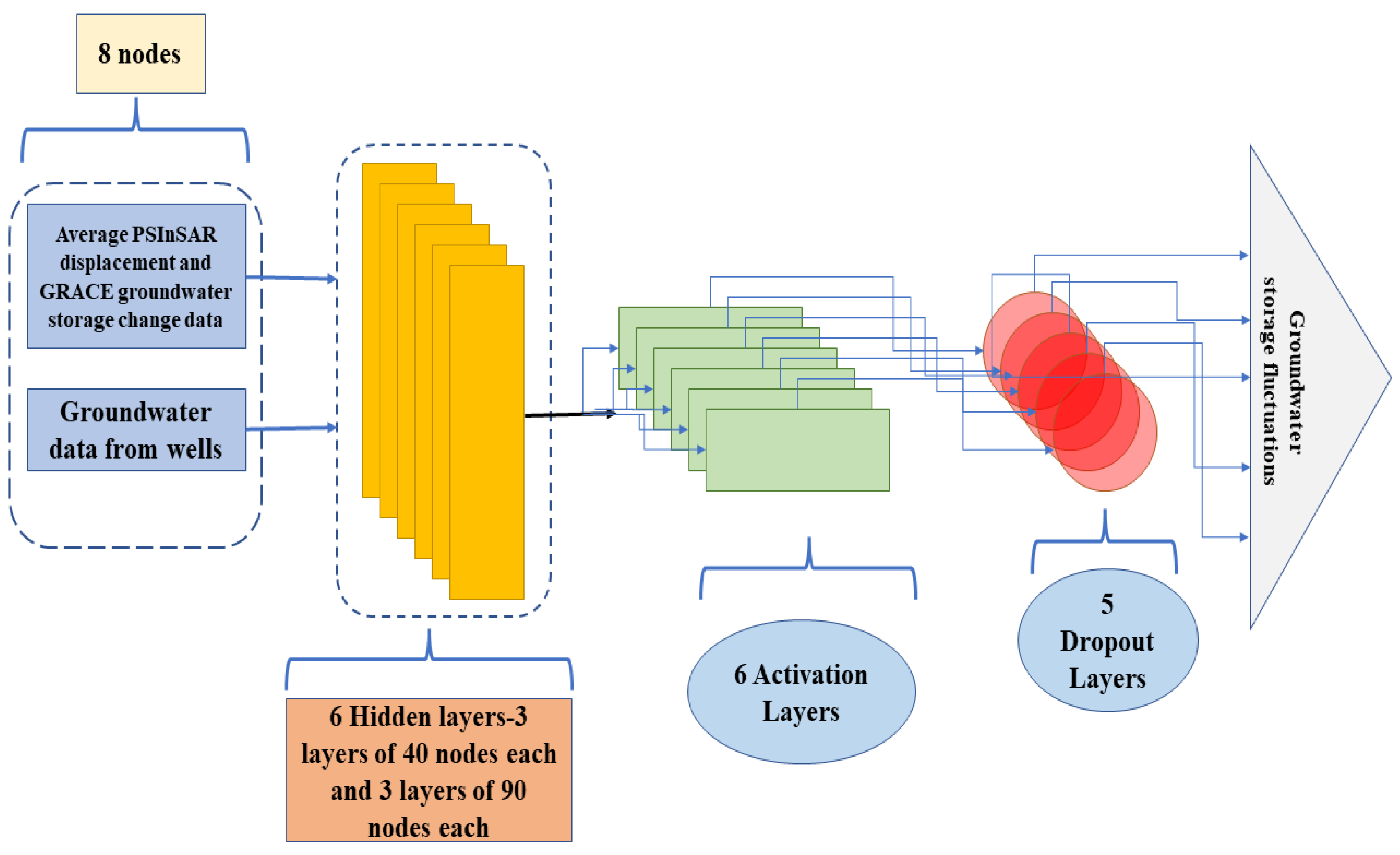
Based on the large number of datasets of the per pixel input from the PSInSAR and inverse distance weighted (IDW) interpolated groundwater well data from different locations of the study area, a DLMLP neural network model was developed as a first of its kind that could estimate ΔGWS at the city level without dwelling in the complex operation of downscaling the GRACE data from 111 km by 111 km spatial resolution, which is not possible beyond a certain point using other statistical techniques. The model comprised six hidden (three layers of 40 nodes, three layers of 90 nodes each), five dropout, and six activation layers. The rectified linear unit (ReLU) was used as the activation function in this model due to its speed of execution and simplicity of implementation [60]. Figure 4 shows the schematic diagram of the DLMLP model used in this study.

3. Results

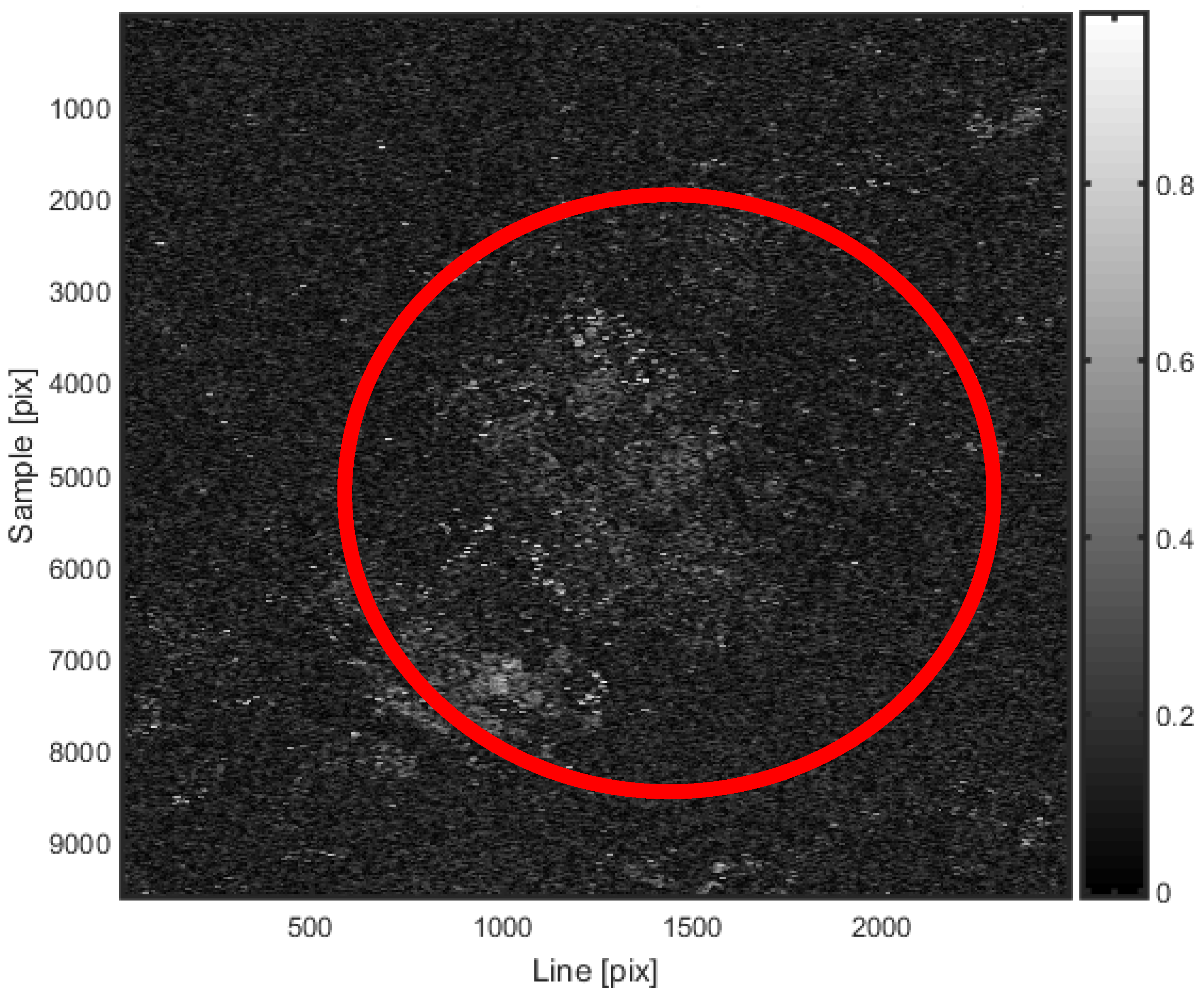
From the coherence analysis of the study area from 2017 to 2022, it was observed that the built-up features were the only coherent features among the other LULC features (as shown in Figure 1). The coherence map has been shown in Figure 5 with built-up features showing high values (close to 1) of coherence. Based on the coherence map (as shown in Figure 5), PS points were selected from the built-up features for a further time series analysis.
The coherence map showing built-up features with coherence values close to 1 is shown in Figure 5.
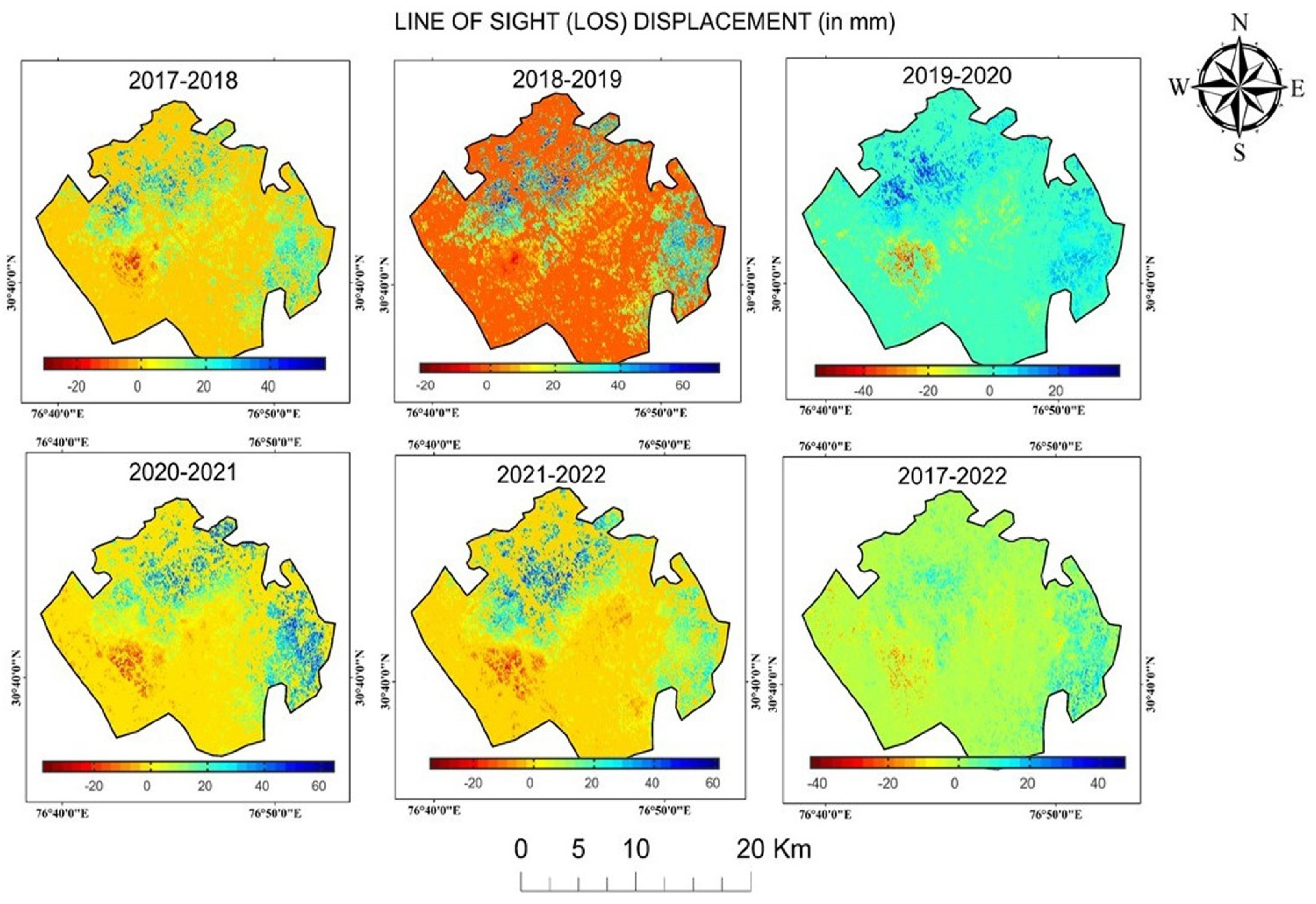
The LOS displacement, indicating the surface subsidence for 2017–18, 2018–19, 2019–20, 2020–21, 2021–22, and 2017–2022, is shown in Figure 6.
From Figure 6, it is observed that there were both positive and negative values of the LOS displacement. The PS points displaced away from the sensor showed negative values while the ones displaced towards the satellite sensor showed positive values. These LOS displacement values accounted for the urban surface subsidence. It is inferred from the above results that the maximum subsidence has been up to 4.0 cm or 40 mm from 2017 to 2022 towards the southwestern part of the study area.
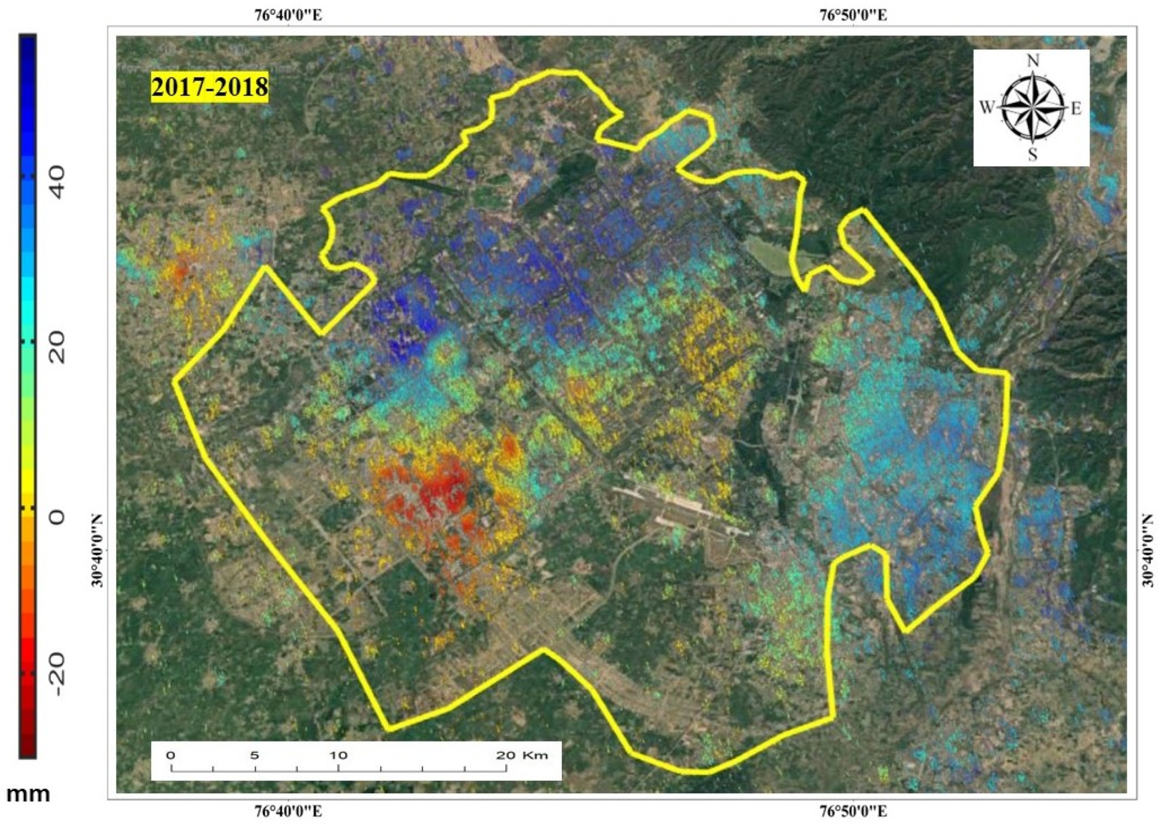
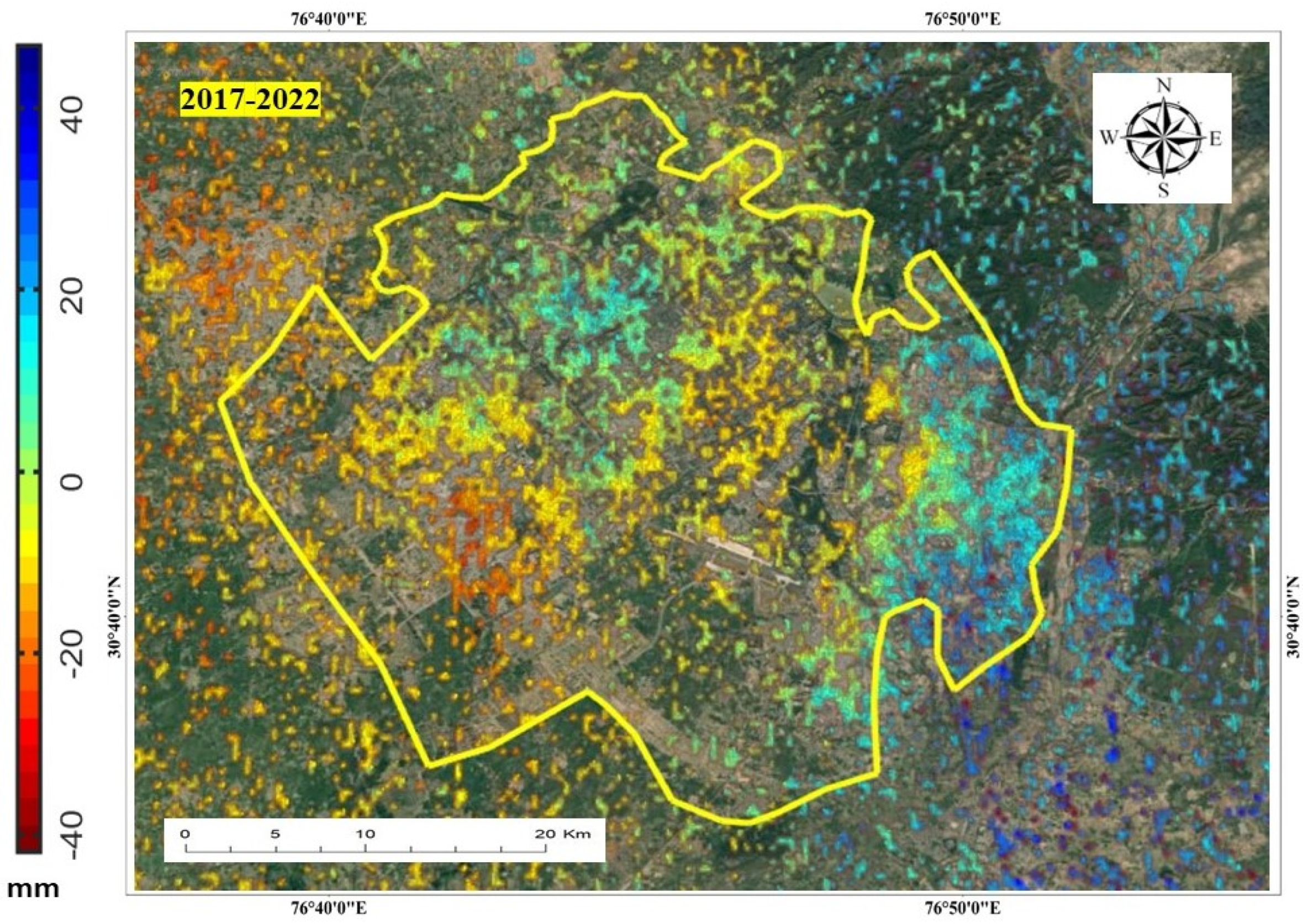
The Google Earth overlays of the urban surface subsidence of the Chandigarh tri-city region are shown in Figure 7.
Apart from the surface displacement mapping of the study region, it is also important to carry out the correlation analysis to check and establish the interoperability of the different data from different sources used in the study. The correlation analysis was carried out through the correlative plots as shown in Figure 8, Figure 9 and Figure 10. The correlative plots for groundwater level fluctuations in the study area and average gravimetric anomaly values are shown in Figure 8.
Figure 8. Correlative plot of groundwater level fluctuations from wells across the study area with GRACE data-based average gravimetric anomaly from 2017 to 2022.
Water 15 01206 g008
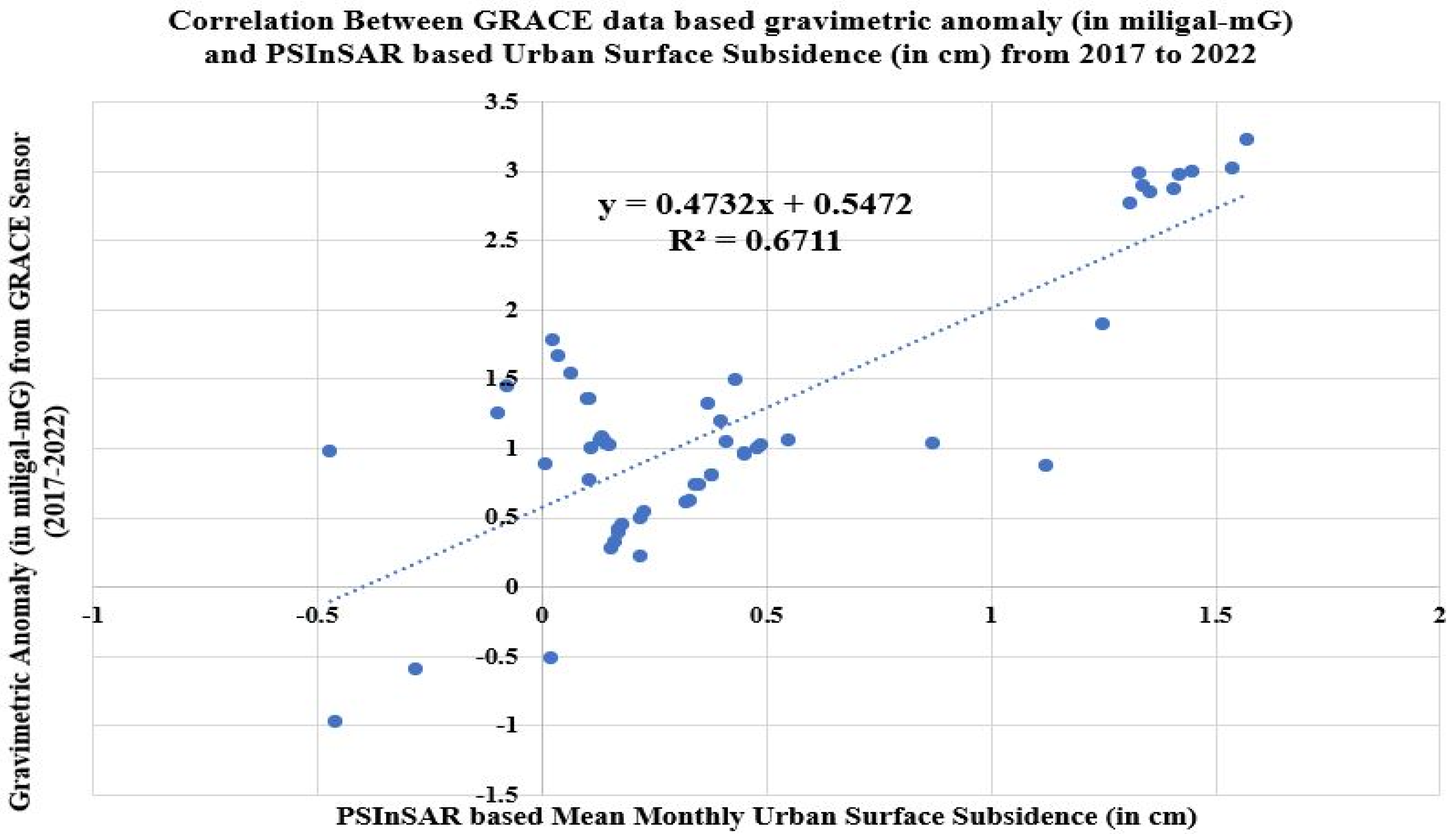
Similarly, the correlative plots of the average PSInSAR values with GRACE data-based gravimetric anomaly and groundwater level data, month-wise from January 2017 to 2022, are shown in Figure 9 and Figure 10.
Figure 9. Correlative plot of average PSInSAR-based urban surface subsidence and groundwater data from wells between 2017 and 2022.
Water 15 01206 g009
Figure 10. Correlation between average GRACE data and average PSInSAR findings from Sentinel-1 SAR data month-wise from 2017 to 2022.
Water 15 01206 g010
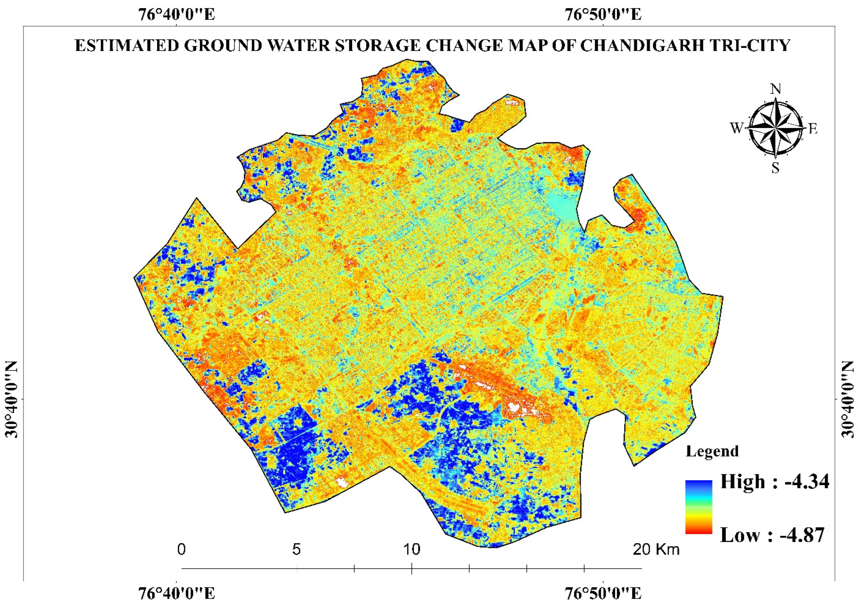
The reason for using gravimetric values directly from GRACE and not ΔGWS in Figure 9 and Figure 10 was only to establish the interoperability of the Sentinel-1 SAR sensor and GRACE satellite sensor. Even if the ΔGWS values were to be used instead of the gravimetric values, the correlation coefficient would have been more than 50%, since the ΔGWS has been derived from the GRACE data using a method as described by Agarwal et al. (2020), Güntner (2008), and Kurtenbach et al. (2009) [59,60,61,62]. In Figure 8, Figure 9 and Figure 10, it is observed that there was a good correlation between the groundwater level data from wells (25 borewells chosen for the data collection) in the study area and satellite data findings of both SAR and GRACE. This forms the basis that the SAR and GRACE sensors had sufficient interoperability. Based on the observations in Figure 7, Figure 8 and Figure 9, the PSInSAR, GRACE, and well data were fed into the DLMLP model as shown in Figure 3. Based on the estimations from the DLMLP model, the ΔGWS map for the entire Chandigarh tri-city was prepared as shown in Figure 11.
From Figure 11, it is inferred that there was a high ΔGWS of up to −4.34 in the southwestern part of the study area where the maximum surface subsidence has been recorded (please refer to Figure 6 and Figure 7). The estimated average of the ΔGWS was found to be −4.605, which was compared with the average ΔGWS (from GRACE and GLDAS LSM).

Time Series Analysis

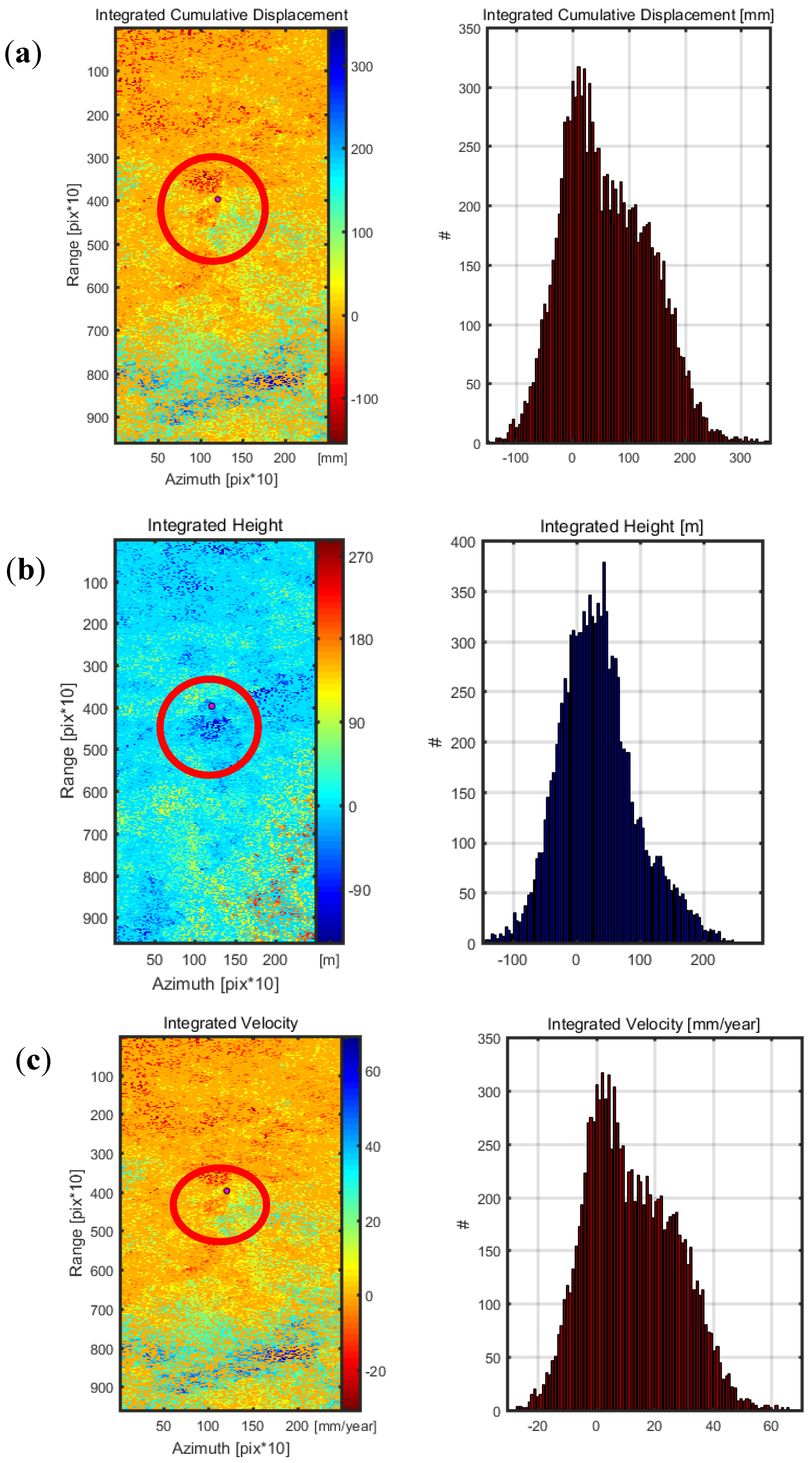
After the APS removal, a detailed time series analysis was carried out for the PSInSAR findings, and based on the coherence values of the built-up, some 7519 coherent or PS points were identified. As explained before in Section 3, these points were stationary with respect to the other points on the same building but dynamic with respect to the ground and each other; therefore, any random point was selected out of the PS points and its cumulative displacement, velocity, and height fluctuation were analyzed in mm/year. The findings are plotted in Figure 12.
The random PS point selected for the time series analysis must be stable with reference to the other points on the same built-up feature (for example, the same building). This was proven by the peaks observed at zero point in the cumulative displacement, height, and velocity graphs as evident in Figure 12. Since SAR interferometry-based LOS displacement is a measure of relative movement to the point of reference, hence the 2nd PS point must be selected as highly stable with high coherence. This was proven in the height histogram with a peak at zero (Figure 12b), which means that the selected PS point was on the ground since points above the ground were known to be relatively unstable. In addition, the peak of the relative velocity histogram should be at zero (Figure 12c); this further confirmed the stability of the selected PS point. The histograms as shown in Figure 12 represent the integrated displacement, height, and velocity of each point with respect to the reference point.
The data from wells and domestic borings, based on the depth the boring had to be increased in the period from 2017 to 2022, are shown in Table 2.
From Table 2, it was observed that there has been a net decline in the groundwater levels in the city, and this was equally evident from the surface subsidence values. However, the real causes need to be identified after a detailed geological investigation only.

4. Discussion

Overpopulation in cities is leading to severe stress on our available urban resources, and there is an acute shortage of open spaces, recreational facilities, and breathable air apart from potable water. Most of the cities located along the banks of rivers in India have depended upon the rivers to meet their water supply requirements. The civic bodies also designed water supply systems based on the population to whom they had to cater. However, with the exponential increase in the population of these cities, many houses and institutional installations came up with unregulated borings to tap the underground water from aquifers. This led to the drying-up of the aquifers, and the decline in average rainfall over the years has not been able to recharge them completely. The recharge deficit has caused the loss in hydrostatic pressure, leading to urban surface subsidence of close to 4.0 cm in five years, which is an alarming situation for a city such as Chandigarh that is in seismic zone IV/V. Therefore, not only is the multi-sensor interoperability of remote sensing data important, as established in this study using the Sentinel-1 SAR and GRACE datasets, but also the estimation and regular monitoring of subsidence and groundwater levels are equally important for safe and sustainable living. It is also important that town planning also takes up resource planning, and unregulated borings and unpermitted settlements should be fined by the authorities. Furthermore, every house or construction coming up should have recharge pits to arrest rainwater and help in the underground aquifer recharge.
Deep learning models are being used with remote sensing data for several classification and regression problems. The deep learning models often solve complex data-related issues which would otherwise be difficult with normal mathematical models. In this study, since satellite data were used from different sensors at different spatial resolutions, it was important to develop a robust model that could give highly accurate estimations. Since satellite sensors have a fixed lifespan, before the launch of a follow-up mission, there could be a data availability gap. Therefore, the relationships between different datasets with which a deep learning model is trained can help in obtaining highly accurate estimates of the data. In addition, since the GRACE and GLDAS LSM data were available at a very coarse spatial resolution, it was difficult to obtain ΔGWS at the city scale. Therefore, a deep learning-based estimation was carried out for ΔGWS which was found to be −4.605 and was very close to the direct satellite data-derived average value of −4.587 for ΔGWS.
Furthermore, the number of layers to be used in a deep learning model depends upon the size of the data. However, being a black box approach, it is still a hit and trial where a number of hidden, activation, and dropout layers is decided based on control of over- and underfitting issues. The number of layers used in this model was found to be optimum to solve the overfitting issues. The ReLu activation function performed better as compared with the other activation function in dealing with outliers. Moreover, the implementation of the ReLu was simple and faster than the other activation functions in model execution, which made it the better choice to be used in the deep learning model for this study.
Additionally, from the results, it was observed that the urban surface subsidence had been up to a maximum of 4.0 cm from 2017 to 2022, and yearly it had been in the range of a maximum of 2.0–4.0 cm. However, in 2019, the flash floods and heavy rains in the Himachal–Punjab region might have caused an aquifer recharge that was reflected in a positive LOS displacement at many places in the north and northeastern Chandigarh tri-city region. It is a good sign of aquifer recharge that it can arrest the surface subsidence to a great extent. It also indicates that a proper green cover and unpaved surface should be left out for the natural recharge of the groundwater.

Points of Difference with a Previous Study by Tripathi et al. (2022) [46]

This study is closely related to the study conducted by Tripathi et al. (2022) [46], where the gravimetric anomaly was estimated using the indirect downscaling method. In that study, the ordinary least squares (OLS) model was used since it is easy and there was a mostly linear relationship observed between the parameters used. However, the outliers and model overfitting are a challenge that needs to be overcome in simple models such as the OLS. In this study of Chandigarh, the major points of difference are the following:
  • Owing to a large amount of per pixel data and a detailed time series analysis for PSInSAR displacement, a more complex machine learning model (the DLMLP) has been used here.
  • This study makes use of GLDAS-LSM data along with the GRACE and Sentinel-1 Satellite datasets.
  • In the study conducted for Varanasi, the change in GRACE data values was an indicator of groundwater fluctuations, while in this study for Chandigarh, surface water has been subtracted to focus more precisely on the groundwater storage changes only.
  • Both Varanasi and Chandigarh are different in their location and geology, as the city of Varanasi has newer alluvium, and still the mighty Ganges is a big source of water supply for the region. For Chandigarh, the situation is more complex since it entirely depends upon the groundwater to meet its water requirements; hence, this study is more crucial.
  • The seismic risks are higher for Chandigarh and surface displacement is more crucial since Chandigarh is in seismic zone IV/V while Varanasi is in seismic zone III. Therefore, this study details the time series analysis more as compared to Varanasi (see Section 2.4.4).

5. Conclusions

The downscaling of coarse resolution data such as GRACE to the city scale has been a challenge for researchers worldwide and often results in a loss of information with conventional downscaling methods. This study presents an indirect downscaling method using average values initially since one pixel of GRACE was larger than the entire study area. The study does not claim for a net-to-net accuracy; however, it has been able to give comparable ΔGWS figures of the average ΔGWS as derived directly from the satellite datasets of GRACE and GLDAS LSM. This shows the high reliability of this deep learning-based approach which could be helpful in data non-availability or a data acquisition gap.
This study is also important since, in the absence of groundwater level data from wells, SAR and GRACE data sensor interoperability can be used as an indicator of groundwater level status in terms of ΔGWS values. Thus, the study also establishes sensor interoperability where the inputs from one sensor such as SAR can be used for the estimation of data which are obtained from the other sensor such as GRACE, despite the two operating at different spatial resolutions. Moreover, with the application of machine learning, it is possible to make accurate estimations of ΔGWS for the future, which would be helpful when the satellite sensor has passed its mission life and there is an observation gap. From the results, it is also observed that it is important for the authorities to decide the maximum population that a planned township can support.
The major novel features and takeaways from the study are as follows:
  • This study establishes that remotely sensed ΔGWS can be used as an indicator of groundwater depletion.
  • The study proves that with the interoperability of SAR and GRACE sensors, regular monitoring of urban surface subsidence and ΔGWS can be carried out.
  • The study also estimates city level ΔGWS using the interoperability of Sentinel-1 SAR and GRACE satellite sensors, which is not possible with the downscaling of a very coarse-resolution GRACE data.
  • The estimated average ΔGWS is observed to be −4.605, and the average from GRACE and GLDAS LSM is observed to be −4.587, which is comparable.
Since the figures are comparable, it can be concluded that the deep learning model performs well. As for the accuracy per pixel, since the datasets used are of very different scales and spatial resolutions, the per pixel accuracy is difficult to obtain.

5.1. Limitations of the Present Study

The study follows an indirect downscaling approach for ΔGWS estimation. In the initial course of the study, monthly average data from GRACE and GLDAS-LSM along with the Sentinel-1 PSInSAR are used to develop a relationship so that a per pixel output of ΔGWS can be estimated later with the per pixel input of PSInSAR. The major limitation here is that there is no means to verify the estimated per pixel ΔGWS values. The only satellite datasets available for this are GRACE and GLDAS-LSM, which are at a very coarse resolution for such a small area.

5.2. Future Work

In the future, rainfall data downscaled to city level from satellite sensors supplemented by on-ground rain gauge data can also be utilized along with PSInSAR-based surface subsidence and GRACE data for a detailed analysis of the groundwater table recharge deficit. This shall draw a clearer picture with higher accuracy of the estimated surface subsidence and ΔGWS over time.
Such studies that use remote sensing and deep learning-based sensor interoperability are highly useful for cities that are dependent upon groundwater for their water demand as they help the civic bodies to plan and regulate the groundwater utilization in an optimum and sustainable manner.

Author Contributions

Conceptualization, A.R.R. and H.A.S.S.; methodology, A.R.R.; software, A.R.R.; validation, A.R.R. and A.T.; formal analysis, A.R.R.; investigation, A.R.R.; resources, H.A.S.S.; data curation, A.R.R.; writing—original draft preparation, A.R.R.; writing—review and editing, A.T. and C.C.; visualization, A.R.R.; supervision, H.A.S.S.; project administration, H.A.S.S. All authors have read and agreed to the published version of the manuscript.

Funding

No funding was received from any source for this research.

Data Availability Statement

The data will be made available by the authors upon reasonable request through proper channel.

Acknowledgments

This study was supported by the Department of Civil Engineering, Punjab Engineering College (PEC) Chandigarh, India; European Space Agency (ESA); Alaska Satellite Facility (ASF), SNAP software team; and Geotronics ltd. Slovakia for SARPROZ software and the SARPROZ software team.

Conflicts of Interest

The authors declare no conflict of interest.

References

  1. Elmes, A.; Alemohammad, H.; Avery, R.; Caylor, K.; Eastman, J.R.; Fishgold, L.; Friedl, M.A.; Jain, M. Accounting for Training Data Error in Machine Learning Applied to Earth Observations. Remote Sens. 2020, 12, 1034. [Google Scholar] [CrossRef] [Green Version]
  2. Choudhury, P.; Gahalaut, K.; Dumka, R.; Gahalaut, V.K.; Singh, A.K.; Kumar, S. GPS measurement of land subsidence in Gandhinagar, Gujarat (Western India), due to groundwater depletion. Environ. Earth Sci. 2018, 77, 770. [Google Scholar] [CrossRef]
  3. Kayhomayoon, Z.; Arya, N.A.; Milan, S.G.; Moghaddam, K.H.; Berndtsson, R. Novel approach for predicting groundwater storage loss using machine learning. J. Environ. Manag. 2021, 296, 113237. [Google Scholar] [CrossRef]
  4. Bai, X.; Surveyer, A.; Elmqvist, T.; Gatzweiler, F.W.; Güneralp, B.; Parnell, S.; Prieur-Richard, A.-H.; Shrivastava, P.; Siri, J.G.; Stafford-Smith, M.; et al. Defining and advancing a systems approach for sustainable cities. Curr. Opin. Environ. Sustain. 2016, 23, 69–78. [Google Scholar] [CrossRef]
  5. Mohamed, M.A.; Anders, J.; Schneider, C. Monitoring of Changes in Land Use/Land Cover in Syria from 2010 to 2018 Using Multitemporal Landsat Imagery and GIS. Land 2020, 9, 226. [Google Scholar] [CrossRef]
  6. Carrillo-Rivera, J.J.; Cardona, A.; Huizar-Alvarez, R.; Graniel, E. Response of the interaction between groundwater and other components of the environment in Mexico. Environ. Geol. 2008, 55, 303–319. [Google Scholar] [CrossRef]
  7. Squeo, F.A.; Aravena, R.; Aguirre, E.; Pollastri, A.; Jorquera, C.B.; Ehleringer, J.R. Groundwater dynamics in a coastal aquifer in north-central Chile: Implications for groundwater recharge in an arid ecosystem. J. Arid. Environ. 2006, 67, 240–254. [Google Scholar] [CrossRef]
  8. Mundepi, A.K.; Lindholm, C.; Kamal. Soft soil mapping using Horizontal to Vertical Spectral Ratio (HVSR) for seismic hazard assessment of Chandigarh city in Himalayan foothills, north India. J. Geol. Soc. India 2009, 74, 551. [Google Scholar] [CrossRef]
  9. Du, Z.; Ge, L.; Li, X.; Ng, A.H.M. Subsidence Monitoring over the Southern Coalfield, Australia Using both L-Band and C-Band SAR Time Series Analysis. Remote Sens. 2016, 8, 543. [Google Scholar] [CrossRef] [Green Version]
  10. Milczarek, W. Application of a small baseline subset time series method with atmospheric correction in monitoring results of mining activity on ground surface and in detecting induced seismic events. Remote Sens. 2019, 11, 1008. [Google Scholar] [CrossRef] [Green Version]
  11. Levien, M. Special economic zones and accumulation by dispossession in India. J. Agrar. Chang. 2011, 11, 454–483. [Google Scholar] [CrossRef]
  12. Hssaisoune, M.; Bouchaou, L.; Sifeddine, A.; Bouimetarhan, I.; Chehbouni, A. Moroccan groundwater resources and evolution with global climate changes. Geosciences 2020, 10, 81. [Google Scholar] [CrossRef] [Green Version]
  13. Perrin, J.; Mascré, C.; Pauwels, H.; Ahmed, S. Solute recycling: An emerging threat to groundwater quality in southern India? J. Hydrol. 2011, 398, 144–154. [Google Scholar] [CrossRef]
  14. Steinhardt, R.; Trafford, B.D. SOME EFFECTS SUB-SURFACE DRAINAGE AND PLOUGHING ON THE STRUCTURE and COMPACTABILITY A CLAY SOIL. J. Soil Sci. 1974, 25, 138–152. [Google Scholar] [CrossRef]
  15. Arthurton, R.S. Marine-related physical natural hazards affecting coastal megacities of the Asia–Pacific region–awareness and mitigation. Ocean. Coast. Manag. 1998, 40, 65–85. [Google Scholar] [CrossRef]
  16. Roccheggiani, M.; Piacentini, D.; Tirincanti, E.; Perissin, D.; Menichetti, M. Detection and monitoring of tunneling induced ground movements using Sentinel-1 SAR Interferometry. Remote Sens. 2019, 11, 639. [Google Scholar] [CrossRef] [Green Version]
  17. Tomás, R.; Romero, R.; Mulas, J.; Marturià, J.J.; Mallorquí, J.J.; López-Sánchez, J.M.; Gutiérrez, F.; González, P.J.; Fernández, J.; Duque, S.; et al. Radar interferometry techniques for the study of ground subsidence phenomena: A review of practical issues through cases in Spain. Environ. Earth Sci. 2014, 71, 163–181. [Google Scholar] [CrossRef] [Green Version]
  18. Strozzi, T.; Wegmuller, U.; Werner, C.L.; Wiesmann, A.; Spreckels, V. JERS SAR interferometry for land subsidence monitoring. IEEE Trans. Geosci. Remote Sens. 2003, 41, 1702–1708. [Google Scholar] [CrossRef]
  19. Dehghani, M.; Zoej, M.J.V.; Hooper, A.; Hanssen, R.F.; Entezam, I.; Saatchi, S. Hybrid conventional and persistent scatterer SAR interferometry for land subsidence monitoring in the Tehran Basin, Iran. ISPRS J. Photogramm. Remote Sens. 2013, 79, 157–170. [Google Scholar] [CrossRef]
  20. Azarakhsh, Z.; Azadbakht, M.; Matkan, A. Estimation, modeling, and prediction of land subsidence using Sentinel-1 time series in Tehran-Shahriar plain: A machine learning-based investigation. Remote Sens. Appl. Soc. Environ. 2022, 25, 100691. [Google Scholar] [CrossRef]
  21. El Kamali, M.; Abuelgasim, A.; Papoutsis, I.; Loupasakis, C.; Kontoes, C. A reasoned bibliography on SAR interferometry applications and outlook on big interferometric data processing. Remote Sens. Appl. Soc. Environ. 2020, 19, 100358. [Google Scholar] [CrossRef]
  22. Cavur, M.; Moraga, J.; Duzgun, H.S.; Soydan, H.; Jin, G. Displacement analysis of geothermal field based on PSInSAR and SOM clustering algorithms a case study of Brady Field, Nevada—USA. Remote Sens. 2021, 13, 349. [Google Scholar] [CrossRef]
  23. Zhang, Y.; Zhang, J.; Wu, H.; Lu, Z.; Guangtong, S. Monitoring of urban subsidence with SAR interferometric point target analysis: A case study in Suzhou, China. Int. J. Appl. Earth Obs. Geoinf. 2011, 13, 812–818. [Google Scholar] [CrossRef]
  24. Ng, A.H.M.; Ge, L.; Du, Z.; Wang, S.; Ma, C. Satellite radar interferometry for monitoring subsidence induced by longwall mining activity using Radarsat-2, Sentinel-1 and ALOS-2 data. Int. J. Appl. Earth Obs. Geoinf. 2017, 61, 92–103. [Google Scholar] [CrossRef]
  25. Liosis, N.; Marpu, P.R.; Pavlopoulos, K.; Ouarda, T.B. Ground subsidence monitoring with SAR interferometry techniques in the rural area of Al Wagan, UAE. Remote Sens. Environ. 2018, 216, 276–288. [Google Scholar] [CrossRef]
  26. Chen, B.; Gong, H.; Lei, K.; Li, J.; Zhou, C.; Gao, M.; Guan, H.; Lv, W. Land subsidence lagging quantification in the main exploration aquifer layers in Beijing plain, China. Int. J. Appl. Earth Obs. Geoinf. 2019, 75, 54–67. [Google Scholar] [CrossRef]
  27. Tiwari, A.; Narayan, A.B.; Dwivedi, R.; Dikshit, O.; Nagarajan, B. Monitoring of landslide activity at the Sirobagarh landslide, Uttarakhand, India, using LiDAR, SAR interferometry and geodetic surveys. Geocarto Int. 2020, 35, 535–558. [Google Scholar] [CrossRef]
  28. Govil, H.; Chatterjee, R.S.; Bhaumik, P.; Vishwakarma, N. Deformation monitoring of Surakachhar underground coal mines of Korba, India using SAR interferometry. Adv. Space Res. 2022, 70, 3905–3916. [Google Scholar] [CrossRef]
  29. Awasthi, S.; Jain, K.; Bhattacharjee, S.; Gupta, V.; Varade, D.; Singh, H.; Narayan, A.B.; Budillon, A. Analyzing urbanization induced groundwater stress and land deformation using time-series Sentinel-1 datasets applying PSInSAR approach. Sci. Total Environ. 2022, 844, 157103. [Google Scholar] [CrossRef]
  30. Cigna, F.; Bateson, L.B.; Jordan, C.J.; Dashwood, C. Simulating SAR geometric distortions and predicting Persistent Scatterer densities for ERS-1/2 and ENVISAT C-band SAR and InSAR applications: Nationwide feasibility assessment to monitor the landmass of Great Britain with SAR imagery. Remote Sens. Environ. 2014, 152, 441–466. [Google Scholar] [CrossRef] [Green Version]
  31. Kalsi, N.; Kiran, R. Greater Mohali Region: Geopolitical Impact on Urban Anthropology to Emerge as a Significant Tri-city Entity. J. Hum. Ecol. 2014, 47, 125–137. [Google Scholar] [CrossRef]
  32. Siddiqui, A.; Kakkar, K.K.; Halder, S.; Kumar, P. Smart Chandigarh Tri-City Region: Spatial Strategies of Transformation. In Smart Metropolitan Regional Development: Economic and Spatial Design Strategies; Kumar, T.M.V., Ed.; Springer: Singapore, 2019; pp. 403–450. [Google Scholar] [CrossRef]
  33. Jain, S.K.; Agarwal, P.K.; Singh, V.P. Groundwater. In Hydrology and Water Resources of India; Jain, S.K., Agarwal, P.K., Singh, V.P., Eds.; Springer: Dordrecht, The Netherlands, 2007; pp. 235–294. [Google Scholar] [CrossRef]
  34. Keesari, T.; Sinha, U.K.; Saha, D.; Dwivedi, S.N.; Shukla, R.R.; Mohokar, H.; Roy, A. Isotope and hydrochemical systematics of groundwater from a multi-tiered aquifer in the central parts of Indo-Gangetic Plains, India–implications for groundwater sustainability and security. Sci. Total Environ. 2021, 789, 147860. [Google Scholar] [CrossRef]
  35. Korisettar, R. Toward developing a basin model for Paleolithic settlement of the Indian subcontinent: Geodynamics, monsoon dynamics, habitat diversity and dispersal routes. In The Evolution and History of Human Populations in South Asia: Inter-disciplinary Studies in Archaeology, Biological Anthropology, Linguistics and Genetics; Petraglia, M.D., Allchin, B., Eds.; Springer: Dordrecht, The Netherlands, 2007; pp. 69–96. [Google Scholar] [CrossRef]
  36. Gargani, J.; Abdessadok, S.; Tudryn, A.; Sao, C.C.; Malassé, A.D.; Gaillard, C.; Moigne, M.-A.; Singh, M.; Bhardwaj, V.; Karir, B. Geology and geomorphology of Masol paleonto-archeological site, Late Pliocene, Chandigarh, Siwalik Frontal Range, NW India. Comptes Rendus Palevol 2016, 15, 379–391. [Google Scholar] [CrossRef] [Green Version]
  37. Kandpal, G.C.; Agarwal, K.K. Assessment of liquefaction potential of the sediments of Chandigarh area. J. Geol. Soc. India 2018, 91, 323–328. [Google Scholar] [CrossRef]
  38. Kadiyan, N.; Chatterjee, R.S.; Pranjal, P.; Agrawal, P.; Jain, S.K.; Angurala, M.L.; Biyani, A.K.; Sati, M.S.; Kumar, D.; Bhardwaj, A.; et al. Assessment of groundwater depletion–induced land subsidence and characterisation of damaging cracks on houses: A case study in Mohali-Chandigarh area, India. Bull. Eng. Geol. Environ. 2021, 80, 3217–3231. [Google Scholar] [CrossRef]
  39. Ferretti, A.; Prati, C.; Rocca, F. Permanent scatterers in SAR interferometry. IEEE Trans. Geosci. Remote Sens. 2001, 39, 8–20. [Google Scholar] [CrossRef]
  40. Sowter, A.; Amat, M.B.C.; Cigna, F.; Marsh, S.; Athab, A.; Alshammari, L. Mexico City land subsidence in 2014–2015 with Sentinel-1 IW TOPS: Results using the Intermittent SBAS (ISBAS) technique. Int. J. Appl. Earth Obs. Geoinf. 2016, 52, 230–242. [Google Scholar] [CrossRef]
  41. Wegnüller, U.; Werner, C.; Strozzi, T.; Wiesmann, A.; Frey, O.; Santoro, M. Sentinel-1 support in the GAMMA software. Procedia Comput. Sci. 2016, 100, 1305–1312. [Google Scholar] [CrossRef] [Green Version]
  42. Tripathi, A.; Attri, L.; Tiwari, R.K. Spaceborne C-band SAR remote sensing–based flood mapping and runoff estimation for 2019 flood scenario in Rupnagar, Punjab, India. Environ. Monit. Assess. 2021, 193, 110. [Google Scholar] [CrossRef]
  43. Upreti, M.; Kumar, D. Investigating capability of open archive multispectral and SAR datasets for Wheat crop monitoring and acreage estimation studies. Earth Sci. Inform. 2021, 14, 2017–2035. [Google Scholar] [CrossRef]
  44. Tripathi, A.; Tiwari, R.K. Synergetic utilization of sentinel-1 SAR and sentinel-2 optical remote sensing data for surface soil moisture estimation for Rupnagar, Punjab, India. Geocarto Int. 2022, 37, 2215–2236. [Google Scholar] [CrossRef]
  45. Aziz, M.A.; Moniruzzaman, M.; Tripathi, A.; Hossain, M.I.; Ahmed, S.; Rahaman, K.R.; Rahman, F.; Ahmed, R. Delineating flood zones upon employing synthetic aperture data for the 2020 flood in Bangladesh. Earth Syst. Environ. 2022, 6, 733–743. [Google Scholar] [CrossRef]
  46. Tripathi, A.; Reshi, A.R.; Moniruzzaman, M.; Rahaman, K.R.; Tiwari, R.K.; Malik, K. Interoperability of-Band Sentinel-1 SAR and GRACE Satellite Sensors on PSInSAR-Based Urban Surface Subsidence Mapping of Varanasi, India. IEEE Sens. J. 2022, 22, 21071–21081. [Google Scholar] [CrossRef]
  47. Tripathi, A.; Tiwari, R.K. Utilisation of spaceborne C-band dual pol Sentinel-1 SAR data for simplified regression-based soil organic carbon estimation in Rupnagar, Punjab, India. Adv. Space Res. 2022, 69, 1786–1798. [Google Scholar] [CrossRef]
  48. Tripathi, A.; Maithani, S.; Kumar, S. Minimization of the ambiguity of merging of urban builtup and fallow land features by generating ‘C2’ covariance matrix using spaceborne bistatic dual Pol SAR data. In Proceedings of the 2018 4th International Conference on Recent Advances in Information Technology (RAIT), Dhanbad, India, 15–17 March 2018; pp. 1–4. [Google Scholar] [CrossRef]
  49. Tripathi, A.; Maithani, S.; Kumar, S. X-band persistent SAR interferometry for surface subsidence detection in Rudrapur City, India. Remote Sens. Technol. Appl. Urban Environ. III SPIE 2018, 10793, 105–115. [Google Scholar] [CrossRef]
  50. Tripathi, A.; Tiwari, R.K. A simplified subsurface soil salinity estimation using synergy of SENTINEL-1 SAR and SENTINEL-2 multispectral satellite data, for early stages of wheat crop growth in Rupnagar, Punjab, India. Land Degrad. Dev. 2021, 32, 3905–3919. [Google Scholar] [CrossRef]
  51. Li, Z.; Cao, Y.; Wei, J.; Duan, M.; Wu, L.; Hou, J.; Zhu, J. Time-series InSAR ground deformation monitoring: Atmospheric delay modeling and estimating. Earth-Sci. Rev. 2019, 192, 258–284. [Google Scholar] [CrossRef]
  52. Talib, O.C.; Shimon, W.; Sarah, K.; Tonian, R. Detection of sinkhole activity in West-Central Florida using InSAR time series observations. Remote Sens. Environ. 2022, 269, 112793. [Google Scholar] [CrossRef]
  53. Chen, J. Satellite gravimetry and mass transport in the earth system. Geod. Geodyn. 2019, 10, 402–415. [Google Scholar] [CrossRef]
  54. Ramillien, G.; Frappart, F.; Seoane, L. Application of the regional water mass variations from GRACE satellite gravimetry to large-scale water management in Africa. Remote Sens. 2014, 6, 7379–7405. [Google Scholar] [CrossRef] [Green Version]
  55. Zencich, S.J.; Froend, R.H.; Turner, J.V.; Gailitis, V. Influence of groundwater depth on the seasonal sources of water accessed by Banksia tree species on a shallow, sandy coastal aquifer. Oecologia 2001, 131, 8–19. [Google Scholar] [CrossRef]
  56. Singh, A.; Seitz, F.; Schwatke, C. Inter-annual water storage changes in the Aral Sea from multi-mission satellite altimetry, optical remote sensing, and GRACE satellite gravimetry. Remote Sens. Environ. 2012, 123, 187–195. [Google Scholar] [CrossRef]
  57. Vishwakarma, B.D.; Zhang, J.; Sneeuw, N. Downscaling GRACE total water storage change using partial least squares regression. Sci. Data 2021, 8, 95. [Google Scholar] [CrossRef]
  58. Castellazzi, P.; Martel, R.; Galloway, D.L.; Longuevergne, L.; Rivera, A. Assessing groundwater depletion and dynamics using GRACE and InSAR: Potential and limitations. Groundwater 2016, 54, 768–780. [Google Scholar] [CrossRef] [PubMed] [Green Version]
  59. Agarwal, V.; Kumar, A.; Gomes, R.L.; Marsh, S. Monitoring of ground movement and groundwater changes in London using InSAR and GRACE. Appl. Sci. 2020, 10, 8599. [Google Scholar] [CrossRef]
  60. Eckle, K.; Schmidt-Hieber, J. A comparison of deep networks with ReLU activation function and linear spline-type methods. Neural Netw. 2019, 110, 232–242. [Google Scholar] [CrossRef]
  61. Kurtenbach, E.; Mayer-Gürr, T.; Eicker, A. Deriving daily snapshots of the Earth’s gravity field from GRACE L1B data using Kalman filtering. Geophys. Res. Lett. 2009, 36, 1–5. [Google Scholar] [CrossRef]
  62. Güntner, A. Improvement of global hydrological models using GRACE data. Surv. Geophys. 2008, 29, 375–397. [Google Scholar] [CrossRef] [Green Version]
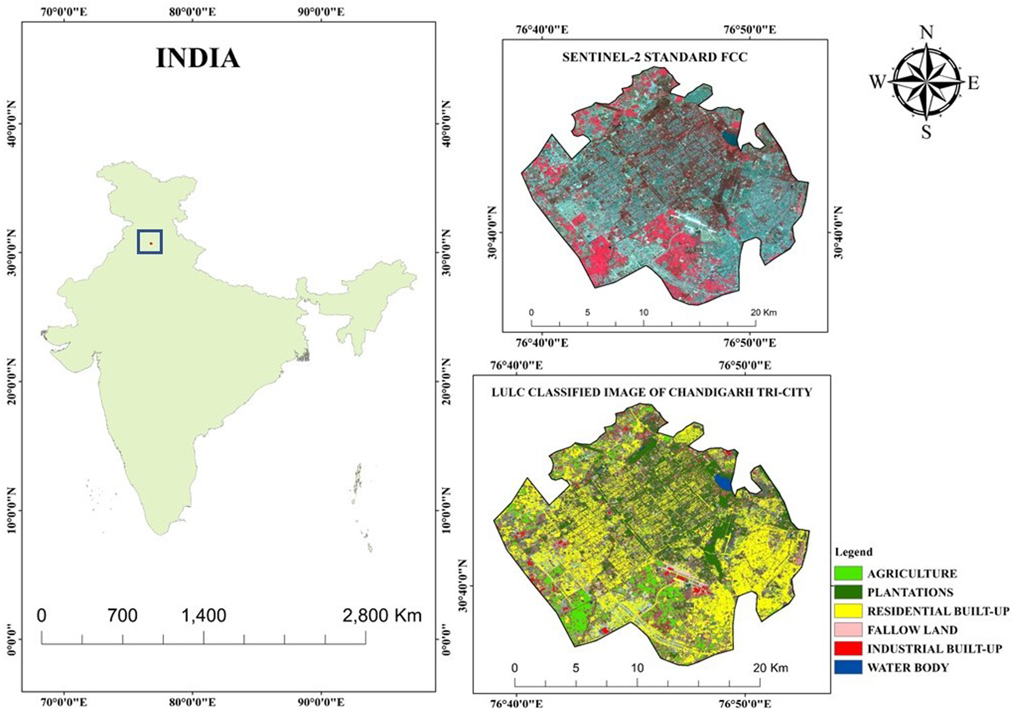
Figure 1. Study area map of Chandigarh showing Sentinel-2 standard false color composite image and land use/land cover classified imagery.
Water 15 01206 g001
Figure 2. Methodology flow diagram.
Water 15 01206 g002
Figure 3. Coherence connection graph.
Water 15 01206 g003
Figure 4. Schematic diagram of the DLMLP model used.
Water 15 01206 g004
Figure 5. Coherence map showing persistent scatterer (built-up) features (in red circle).
Water 15 01206 g005
Figure 6. LOS displacements (in mm) for different time frames from 2017 to 2022.
Water 15 01206 g006
Figure 7. Google Earth overlays of urban surface subsidence maps from 2017 to 2022 in different time frames.
Water 15 01206 g007aWater 15 01206 g007bWater 15 01206 g007cWater 15 01206 g007d
Figure 11. Estimated gravimetric anomaly map for Chandigarh tri-city (in mGAL).
Water 15 01206 g011
Figure 12. Graph plots for PS Point as shown in Red Circle (a) integrated cumulative displacement (in mm), (b) height of the PS point under study (in m), and (c) cumulative velocity from 2017 to 2022 (in mm/year).
Water 15 01206 g012
Table 1. Datasets used.
SL.No.DatasetsPolarizationPeriod
1.Sentinel-1 SAR Single Look Complex (SLC) dataVV+VH Ascending (26 images) and Descending pass (26 images)2017–2022
2.Groundwater level data from CGWB--------2017–2022
3.GRACE monthly terrestrial water storage data--------2017–2022
4.GLDAS LSM soil moisture and surface water --------2017–2022
Table 2. Groundwater data from field and surface displacement.
S.No.Area/Location of Well/Domestic BoringPSInSAR-Based Surface Displacement (in mm) 2017–2022Reported Groundwater Level (mbgl) in 2017 from Field Data CollectionReported Groundwater Level in 2022 from Field Data Collection
1.Sector-43−404041
2.Airport area−372022
3.Sector-12 PEC Campus−332527
4.Sector-17303738
5.Sector- 33253639
6.Sector-29−281516
7.Sector-39−241215
8.Sector-20−221014
9.Sector-7−3557
10.Sector-47−312122
Disclaimer/Publisher’s Note: The statements, opinions and data contained in all publications are solely those of the individual author(s) and contributor(s) and not of MDPI and/or the editor(s). MDPI and/or the editor(s) disclaim responsibility for any injury to people or property resulting from any ideas, methods, instructions or products referred to in the content.