Forecasting Long-Series Daily Reference Evapotranspiration Based on Best Subset Regression and Machine Learning in Egypt

Abstract

The estimation of reference evapotranspiration (ET_o), a crucial step in the hydrologic cycle, is essential for system design and management, including the balancing, planning, and scheduling of agricultural water supply and water resources. When climates vary from arid to semi-arid, and there are problems with a lack of meteorological data and a lack of future information on ET_o, as is the case in Egypt, it is more important to estimate ET_o precisely. To address this, the current study aimed to model ET_o for Egypt’s most important agricultural governorates (Al Buhayrah, Alexandria, Ismailiyah, and Minufiyah) using four machine learning (ML) algorithms: linear regression (LR), random subspace (RSS), additive regression (AR), and reduced error pruning tree (REPTree). The Climate Forecast System Reanalysis (CFSR) of the National Centers for Environmental Prediction (NCEP) was used to gather daily climate data variables from 1979 to 2014. The datasets were split into two sections: the training phase, i.e., 1979–2006, and the testing phase, i.e., 2007–2014. Maximum temperature (T_max), minimum temperature (T_min), and solar radiation (SR) were found to be the three input variables that had the most influence on the outcome of subset regression and sensitivity analysis. A comparative analysis of ML models revealed that REPTree outperformed competitors by achieving the best values for various performance matrices during the training and testing phases. The study’s novelty lies in the use of REPTree to estimate and predict ET_o, as this algorithm has not been commonly used for this purpose. Given the sparse attempts to use this model for such research, the remarkable accuracy of the REPTree model in predicting ET_o highlighted the rarity of this study. In order to combat the effects of aridity through better water resource management, the study also cautions Egypt’s authorities to concentrate their policymaking on climate adaptation.

1. Introduction

Evapotranspiration is the sum of evaporation from the ground surface plus transpiration from plants, and it represents the amount of water required by plants over time. It is vital to the calculation and scheduling of irrigation water in the region and is one of the most influential hydrological factors affecting a region’s climate. This variable must be monitored before agricultural activities on a field may commence. Thus, it is essential for agricultural water supply administrators and users to estimate it accurately. The food and agriculture organization (FAO) standardized a method of Penman–Monteith 56 (FAO PM-56) that estimates reference evapotranspiration (ET_o) using various meteorological data. The World Meteorological Organization (WMO) and the International Commission on Irrigation and Drainage (ICID) introduced the model as a reliable method for estimating ET_o, and it was also approved as a suitable alternative to lysimeter data by the ICID [1]. One of the most significant issues in hydrology and agriculture is ET_o modeling, which allows for the prediction of future values of this variable. In fact, the forecast of this variable tells us how much water the plant will need in the future. This method is quite successful and is used in the region to schedule crop irrigation. Increased demand for limited water resources, climate change, and certain agricultural commodities have all pointed to the need for better ways to make efficient use of the water resources at our fingertips as well as distribute them at the right time and through the right channel to produce premium food [2]. Certain management actions, crop characteristics, weather conditions, land type, and field operations are all key variables that influence the ET_o process [3].

The ability to model ET_o is critical in determining agricultural irrigation requirements on a regional and global scale, preparing water budgets, and assessing the impact of various climatic changes [4]. Significant problems arise when ET_o modeling is tried to estimate accurately using available meteorological data at different gauging stations [5]. A precise measurement of the ET_o serves a variety of purposes including not only the research of climate change and the evaluation of water resources but also the efficient monitoring and forecasting of droughts as well as the correct use and development of water resources [6]. Machine learning (ML) models based on robust algorithms are now being used to map nonlinear processes employing input and output (target) variables. Raza et al. [7] examined research publications on ET_o estimation published in the last eight years (2012–2020) for accuracy, structure, and usefulness. The presented studies’ main goal is to establish an alternative ML model to the FAO-PM56 since it requires a substantial quantity of climatic data as input, which is not accessible at many stations, especially in developing countries. As a result, designing ML models employing all of the usable data comparable to FAO-PM56 is not worthwhile. Moreover, a limited number of studies have investigated the development of a generalized ET_o model for accurate ET_o estimation in all stations within a region, such as Raza et al. [8]. This is particularly important in developing countries since climatic data from most stations are either missing or unavailable owing to technical challenges and a lack of technology. As a result, developing an ET_o model with fewer climatic inputs (such as temperature data) should be enough.

Different types of ML algorithms such as support vector machine (SVM) [9,10], least square support vector machine [11], genetic programming [12,13,14], extreme learning machine (ELM) [15,16], tree-based models [17,18] such as M5 model tree [19,20,21], random forest [22,23,24,25], and extreme gradient boosting (XGBoost) [10,19,26], artificial neural networks (ANNs) [27,28,29], and an adaptive neuro-fuzzy inference system (ANFIS) [30,31] were used in ET_o modeling for this purpose. Utilizing alternative ML models, it may be possible to incorporate such inputs (simultaneously) into the daily ET_o estimation.

According to the available literature, there is no comparison research in the literature that uses random subspace (RSS), additive regression (AR), reduced error pruning tree (REPTree), and linear regression (LR) algorithms to estimate ET_o in the study area of Egypt using daily time-scale data. As a result, this study aims to (i) investigate the historical distributions of ET_o from 1979 to 2014, (ii) evaluate the performance and accuracy of ML algorithms in daily ET_o estimation, and (iii) select the optimal ET_o ML model based on statistical metrics results. These data are essential for understanding the influence of climate change on ET_o in the study region.

2. Materials and Methods

2.1. Study Area

The Nile Delta is Egypt’s economic and financial core and contains the country’s richest agriculture. It is home to eleven governorates. Like the rest of Egypt, the Nile Delta has a hot desert environment. The delta’s warmest months are July and August, when temperatures reach a maximum average of 34 °C. During the winter, temperatures typically range from 9 °C to 19 °C. The annual rainfall is 100–200 mm, with most falling during the winter. Egypt is considered an arid region with a significant danger of water scarcity in the near future. The agricultural sector requires a large amount of water, accounting for around 85 percent of overall freshwater consumption. The study area includes four governorates in Egypt: Al Buhayrah, Alexandria, Ismailiyah, and Minufiyah (Figure 1). These four governorates are located in the Nile Delta, the northern part of Egypt. The Al Buhayrah governorate is located in an important strategic place, west of the Rosetta branch of the Nile River, about 123 km northwest of Cairo, and covers an area of 9826 km². The Alexandria governorate is located in the northern part of the country, directly on the Mediterranean Sea, making it one of the most important harbors in Egypt. The Alexandria governorate is located about 188.6 km northwest of Cairo and covers an area of 2818 km². The Ismailiyah governorate is one of the Canal Zone governorates of Egypt. Located in the northeastern part of the country, it covers an area of 5066 km² and is about 122.5 km away from Cairo. The Minufiyah governorate is located in the Nile Delta’s northern part, north of Cairo. It covers about 2543 km². The population of Al Buhayrah, Alexandria, Ismailiyah, and Minufiyah governorates are estimated by the Central Agency for Public Mobilization and Statistics in Egypt (CAPMAS) [32] to be 6,723,269; 5,469,480; 1,419,631; and 4,640,003 people per capita on 1 January 2022.

2.2. Datasets Description

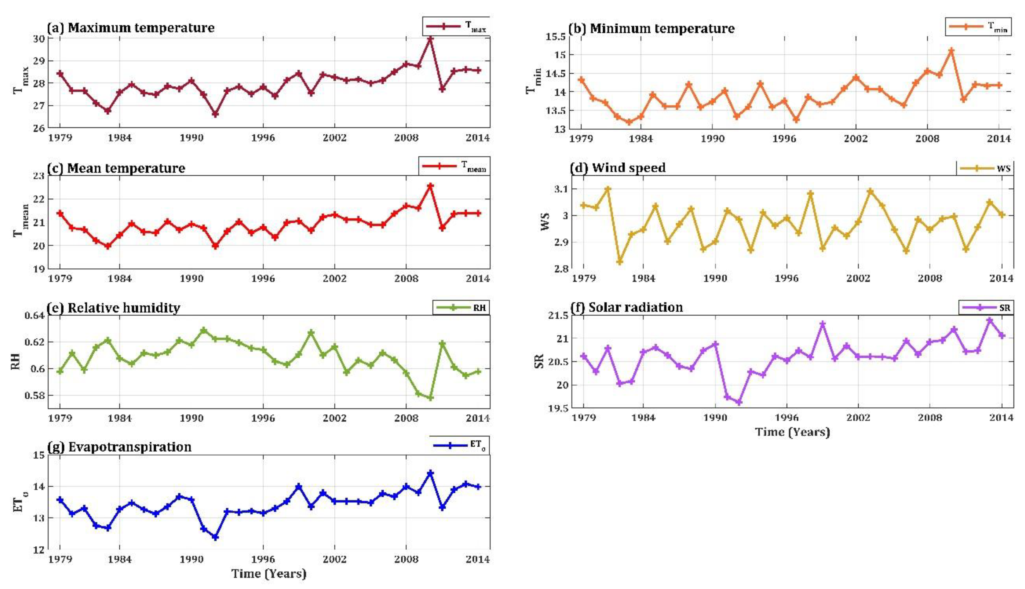
Daily climate data variables for the studied regions, such as minimum and maximum temperatures, humidity, wind speed, vapor pressure deficit, and solar radiation, were collected from the National Centers for Environmental Prediction (NCEP) Climate Forecast System Reanalysis (CFSR) from 1979 to 2014. It was completed over 36 years from 1979 through 2014. Figure 2 demonstrates the time series of each variable for the period 1979–2014. The CFSR was designed and executed as a global, high-resolution, coupled atmosphere-ocean-land surface-sea-ice system to provide the best estimate of the state of these coupled domains over this period. The daily CFSR data (precipitation, wind, relative humidity, and solar radiation) were downloaded in SWAT file format and CSV for the entire period in a zip file by continent.

Table 1. Statistical analysis of climate data variables from 1979 to 2014 in the governorates of Al Buhayrah, Alexandria, Ismailiyah, and Minufiyah.

Governorate	Metrics	Tmax (°C)	Tmin (°C)	Tmean (°C)	P (mm)	WS (Km/h)	RH (%)	SR (kWh/m2)	ETo (mm/day)
Al Buhayrah	Maximum	47.59	26.38	35.09	40.50	9.14	0.98	30.68	34.01
	Minimum	8.17	−2.69	6.36	0.00	0.75	0.11	0.00	0.00
	Average	27.52	13.89	20.71	0.34	3.29	0.64	20.45	13.05
	Std. deviation	6.81	5.28	5.72	1.50	0.92	0.10	7.84	6.83
	Variance	46.40	27.84	32.70	2.24	0.84	0.01	61.53	46.70
	Skewness	−0.21	−0.20	−0.15	8.84	0.96	−0.98	−0.51	−0.06
	Kurtosis	−0.93	−0.97	−1.20	118.55	2.43	2.41	−0.89	−1.13
Alexandria	Maximum	43.43	29.82	35.15	32.97	12.88	0.94	30.49	29.83
	Minimum	9.35	2.72	7.87	0.00	1.20	0.10	0.00	0.00
	Average	26.11	15.98	21.04	0.38	4.52	0.64	20.48	11.28
	Std. deviation	6.06	4.81	5.18	1.53	1.35	0.10	7.82	5.83
	Variance	36.72	23.17	26.82	2.33	1.83	0.01	61.13	33.98
	Skewness	−0.19	−0.08	−0.12	7.69	1.01	−1.43	−0.53	−0.06
	Kurtosis	−0.93	−1.09	−1.21	83.65	2.33	3.14	−0.84	−1.03
Ismailiyah	Maximum	47.76	27.64	35.59	33.74	4.98	0.96	30.74	32.82
	Minimum	7.06	−0.14	5.83	0.00	0.49	0.07	0.00	0.00
	Average	28.81	12.78	20.79	0.18	1.70	0.59	20.71	14.49
	Std. deviation	7.50	4.57	5.74	1.03	0.43	0.12	7.33	7.62
	Variance	56.18	20.87	32.95	1.06	0.18	0.01	53.75	58.14
	Skewness	−0.24	−0.11	−0.15	13.61	1.44	−0.72	−0.42	0.02
	Kurtosis	−1.03	−0.96	−1.18	281.36	5.21	0.97	−0.98	−1.24
Minufiyah	Maximum	48.09	25.30	35.55	60.28	6.38	0.97	31.06	34.41
	Minimum	6.77	−2.23	5.29	0.00	0.62	0.09	0.00	0.00
	Average	29.42	12.84	21.13	0.16	2.36	0.57	20.92	15.00
	Std. deviation	7.74	5.34	6.28	1.01	0.63	0.13	7.43	7.82
	Variance	59.94	28.52	39.43	1.02	0.39	0.02	55.18	61.21
	Skewness	−0.23	−0.23	−0.17	25.06	0.78	−0.36	−0.44	−0.02
	Kurtosis	−1.07	−1.00	−1.23	1134.97	1.95	0.37	−0.97	−1.28

Note: Tmax, maximum temperature; Tmin, minimum temperature; Tmean, mean temperature; WS, wind speed; SR, solar radiation.

presents a statistical analysis of climate data variables in the governorates of Al Buhayrah, Alexandria, Ismailiyah, and Minufiyah from 1979 to 2014.

3. Methodology

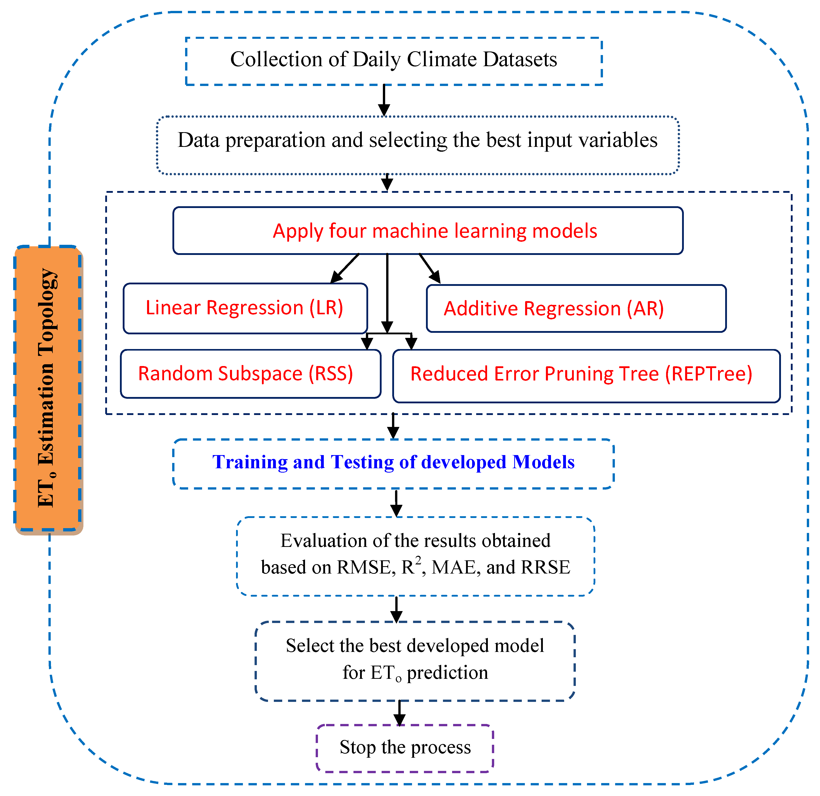
The proposed model for ET_o estimation methodology in the study (Figure 3) is based on the following: (i) collection of daily databases; (ii) data preparation and selection of the best variables; (iii) application of four forecasting machine learning models: linear regression (LR), additive regression (AR), random subspace (RSS), and reduced error pruning tree (REPTree); (iv) training and testing of developed models; (v) evaluation of the results obtained based on RMSE, R², MAE, and RRSE; (vi) selection of the best developed model for ET_o prediction; and finally, (vii) the end of the process. The four forecasting machine learning models used in this study are discussed below:

3.1. Machine Learning (ML) Models

3.1.1. Random Subspace (RSS)

The RSS is a technique for the collective knowledge approach; it is used to investigate arrangement and regression. This model has been applied in land-use categorization, hydrology, irrigation scheduling, evaporation measurement, and forest and agricultural classification [33]. It is an ensemble classifier technique that Ho [34] proposed. In the RSS, the training data are modified. However, this data modification is carried out in the feature space. Hence, each training incidence X_i (i = 1, …, n) in the training sample set X = [X1; …; Xn] is defined as a p-dimensional vector Xi = (x_i1, x_i2, …, x_ip) and defined by p features. Then, r < p features are randomly selected from the p-dimensional dataset X. Consequently, the modified training set X_˜b = X^˜b₁, X^˜b₂…, X^˜b_n, is composed of r-dimensional training incidences. After this step, classifiers are built into the random subspaces X^˜b and aggregated by utilizing a majority voting. Therefore, the RSS is implemented in the following way [35]:

• Repeat for b = 1, 2, …, B;
• Choose an r-dimensional random subspace Xb˜;
• from the original p-dimensional feature space X;
• Build a classifier C^b(x) (with a decision boundary C^b(x) = 0) in Xb˜;
• Aggregate classifiers C^b(x), b = 1, 2, …, B, by utilizing majority voting for the final decision.

The RSS can benefit from using random subspaces for both building and combining the classifiers. When the number of training incidences is comparatively small compared to the data dimension, the small sample size problem can be solved by building classifiers in random subspaces. The subspace dimension will be less than the original feature space, while the number of training incidence is kept the same. Thus, the relative training sample size increases. Once the data have several redundant features, a better classifier can be found in random subspaces than in the original feature space. The aggregated decision of such classifiers might be better than a single classifier built on the original training set in the entire feature space [36]. The parameters used in this model were as follows: batch size—100, classifier—REPTree, random seed—1, subspace size—0.5, number of execution slots—1, number of iterations—10.

3.1.2. Additive Regression (AR)

Regression estimation and variable selection are two important tasks for high-dimensional data mining [37]. Sparse additive models aiming to deal with the above tasks simultaneously have been extensively investigated in the mean regression setting. As a class of models between linear and non-parametric regression, these methods inherit the flexibility from nonparametric regression and the interpretability from linear regression [38]. the generalized additive model (GAM) was constructed by Hastie and Tibshiran [39], which is an extension of the generalized linear model (GLM). The GLM model implies that the parameters are linear, but the GAM model assumes that there is no dependency and that the connection is not necessarily linear [40]. Linear dependence is substituted in that model with broader dependency characteristics [41].

The algorithm’s equation is as follows:

$$g(E\left(y\right))={{\beta }_0+f}_1{x}_1+f_2{x}_2+\cdots +f_p{x}_p+\epsilon$$

(1)

For each single explanatory vector $x_i$, the computation of the application of this model comprises the nonlinear smooth functions $f_i{(x}_i)$, i = 1, …, p.

Several dataset split features are chosen using the standard deviation error (SDR) as a parameter for the optimum characteristics to divide the data set into each node. The chosen attribute is meant to reduce mistakes.

$$\mathrm{SDR}=SD\left(Tree\right)-\mathsf{Ʃ}\frac{Tre{e}_i}{Tree}\mathrm{\ast }SD(Tre{e}_i)$$

(2)

where $Tre{e}_i$ is the subset of cases containing the product of the potential evaluations, and SD (·) denotes the standard deviation of the argument. The stop conditions are either the number of occurrences remaining to accomplish a specific number or a minor type value change.

Table 2. Analysis of best subset regression for determining the best input combinations.

No. of Variables	Variables	MSE	R2	Adjusted R2	Mallows’ Cp	Akaike’s AIC	Schwarz’s SBC	Amemiya’s PC
1	SR	7.670	0.853	0.853	178,771.227	105,837.493	105,855.209	0.147
2	Tmax/SR	2.773	0.947	0.947	31,471.556	52,988.983	53,015.557	0.053
3	Tmax/Tmean/SR	1.728	0.967	0.967	26.095	28,408.184	28,443.616	0.033
4	Tmax/Tmean/RH/SR	1.727	0.967	0.967	4.195	28,386.287	28,430.577	0.033
5 *	Tmax/Tmin/RH/SR	1.727	0.967	0.967	4.195	28,386.287	28,430.577	0.033
6	Tmax/Tmin/WS/RH/SR	1.727	0.967	0.967	6.000	28,388.092	28,441.240	0.033

Note: * The best model for the selected selection criterion is displayed in bold blue. As the number of requested variables could not be entered into the model, the results are unreliable, and the model is not necessarily the best one.

displays the parameters that were used for technique. Parameters selected for applying this method were as follows: batch size—100, classifier—bagging, shrinkage—1, number of iterations—30.

3.1.3. Reduced Error Pruning Tree (REPTree)

The REPTree process is a basic decision tree beginning method that designs and utilizes condensed error trimming to create a regression tree using variance data [42]. As a fast decision tree approach, the REPTree classifier is based on the idea of calculating information acquisition with entropy and minimizing the error caused by variance [43]. The REPTree creates multiple trees in regression tree modified iterations. Then, the best of the trees produced is selected. This algorithm creates a regression/decision tree within the variance framework and the knowledge gain approach. By using the method of linking, this algorithm reduces the pruning error rate. The measure used in pruning the tree is the error in the average frame predicted by the tree. The values of numerical attributes are sorted at the beginning of the modeling process. As with the C4.5 algorithm, this algorithm divides the corresponding samples into pieces and processes the missing values [44].

For numeric characteristics, the algorithm only examines values once. It is primarily the method of constructing a common set of decision-making instructions using a forecaster variable quantity [45,46]. The REPTree decision algorithm is a highly fast learning technique with a low-error pruning tree. It builds a decision/regression tree and prunes it using back-fitting with reduced error based on the data gain/variance [47]. The model’s parameters were as follows: batch size—100, initial count—0, number of folds—3, random seed—1, minimum proportion of the variance—0.001, minimum number—2, maxdepth—1.

3.1.4. Linear Regression (LR)

Linear regression is a potent method for analyzing data in diverse fields [48]. LR predicts a variable’s value based on another variable’s value. The linear regression (LR) model is utilized in numerous application areas [49]: for example, engineering, economics, ecological, social sciences, and medicines, among many others. Hence, linear regression is a powerful and flexible technique to address regression issues. Thus, the trend of the LR model is an extensive topic of significant interest for researchers [50,51]. The parameters selected for implementing this model were as follows: attribute selection method—M5 method; batch size—100; eliminate co-linear attributes—true.

3.2. Performance Metrics

Five performance indicators were employed to evaluate the performances of the applied algorithm as follows: mean absolute error (MAE), mean absolute error (MAE), root mean square error (RMSE), relative absolute error (RAE), root relative squared error (RRSE), and correlation coefficient (R). These parameters were determined using the following equations:

$$MAE=\frac{1}{N}\sum _{i=1}^N\left|X_i-Y_i\right|$$

(3)

$$MSE=\frac{1}{N}\sum _{i=1}^N{\left(X_i-Y_i\right)}^2$$

(4)

$$RMSR=\sqrt{\frac{1}{N}\sum _{i=1}^N{\left(X_i-Y_i\right)}^2}$$

(5)

$$RAE=\left|\frac{X_i-Y_i}{Y_i}\right|\times 100$$

(6)

$$RRSE=\frac{\sqrt{{\sum }_{i=1}^N{\left(Y_i-X_i\right)}^2}}{\sqrt{{\sum }_{i=1}^N{\left(X_i-\stackrel{-}{X}\right)}^2}}$$

(7)

$$R=\frac{{\sum }_i^N\left(X_i-\stackrel{-}{X}\right)\left(Y_i-\stackrel{-}{Y}\right)}{\sqrt{{\sum }_i^N{\left(X_i-\stackrel{-}{X}\right)}^2{\sum }_i^N{\left(Y_i-\stackrel{-}{Y}\right)}^2}}$$

(8)

where N is the total number of measurements; X_i is the observed values, and Y_i is the estimated values; $\stackrel{-}{X}$ is the mean of observed values in X variables; $\stackrel{-}{Y}$ is the mean of estimated values in Y variables.

4. Results

4.1. Analysis of Best Subset Regression for Determining Best Input Combinations

Determining the best input parameters is necessary to achieve the best performance of the selected models. This requires varying combinations of meteorological parameters for shortlisting the best input combinations. The present study aims to develop a joint model for the four study sites (stations), i.e., Alexandria, Al Buhayrah, Minufiyah, and Ismailiyah of Egypt. Shortlisting the best input combinations for the developed models was conducted using the six statistical criteria, i.e., MSE, R², adjusted R², Mallows’ Cp, Akaike’s AIC, Schwarz’s SBC, and Amemiya’s PC, whose results are shown in Table 2. It can be inferred that four input variables, i.e., T_max, T_min, RH, and SR (displayed in bold), were identified as the best input combination given they had the lowest values of Mallows’ Cp (4.195) and Amemiya’s PC (0.033) and the highest value of R² (0.967) and adjusted R² (0.967) amid all input combinations.

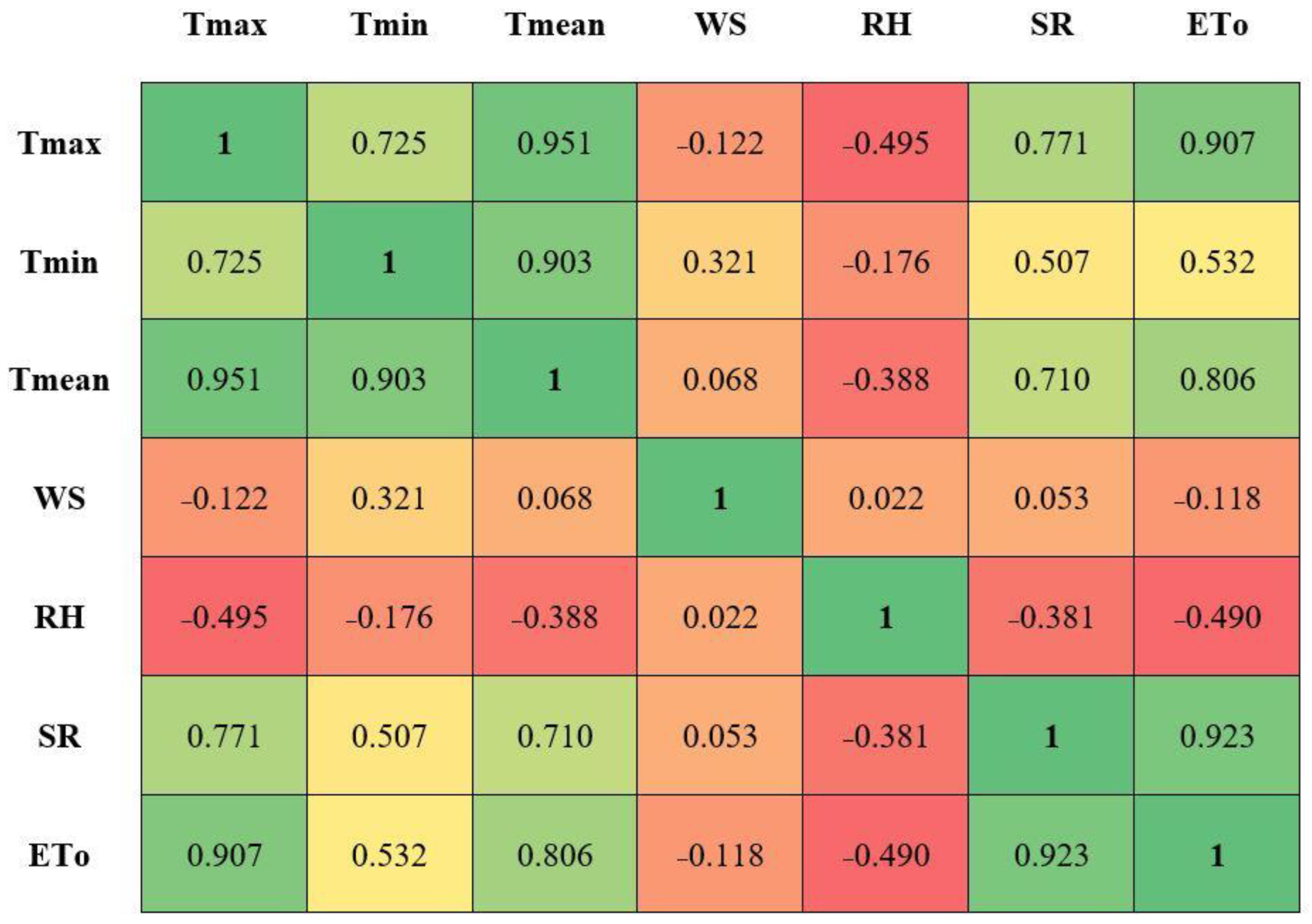
Furthermore, this study conducted correlation analysis to ascertain variable correlations, as shown in Figure 4. In general, the study recorded significantly higher correlations of independent variables with the dependent variable ET_o, for example, 0.907 with T_max, 0.806 with T_mean, and 0.923 with SR. To take advantage of long-term time-series datasets for ET_o, the present study categorized the complete dataset into two sets, of which the first segment comprised 75% of the dataset for training purposes (for the training period 1979–2006), while the second segment comprised 25% for validation/testing purposes (for the testing period 2007–2014) of the models.

4.2. Sensitivity Analysis

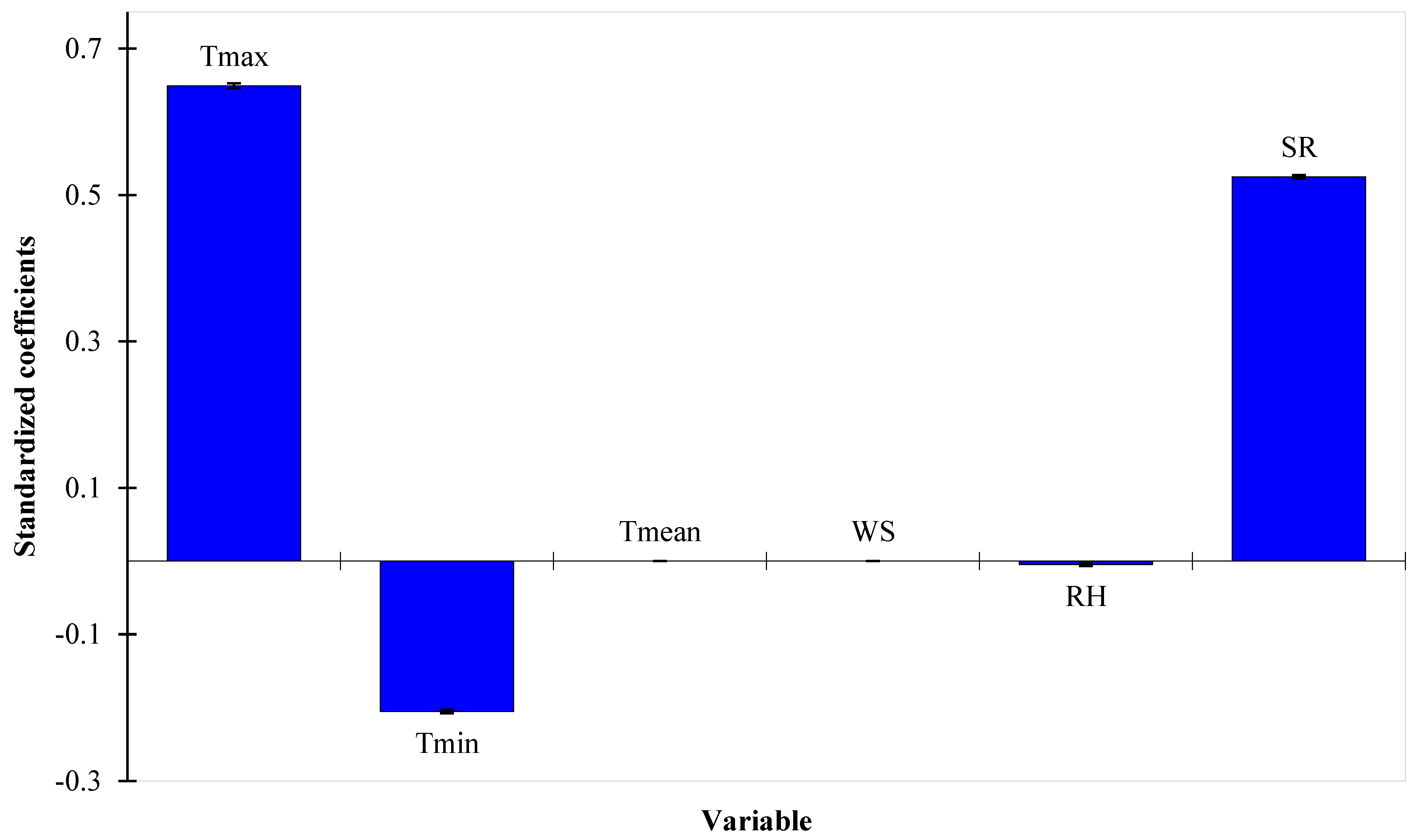
The different combinations of input variables provided the performance of the models such that some combinations yielded positive contributions to the accuracy, while some yielded negative contributions under each case of the selected models. Sensitivity analysis was conducted to shortlist the best influential variables so as to identify the best performance of the models in predicting the ET_o with greater accuracy. Findings from regression analysis on all input variables are summarized in

Table 3. Regression analysis for identifying the most effective parameters for ET_o.

Source	Value	Standard Error	t	Pr > |t|	Lower Bound (95%)	Upper Bound (95%)
Tmax	0.649	0.002	366.370	<0.0001	0.646	0.653
Tmin	−0.205	0.001	−167.137	<0.0001	−0.208	−0.203
Tmean	0.000	0.000
WS	0.000	0.000
RH	−0.005	0.001	−4.889	<0.0001	−0.007	−0.003
SR	0.525	0.001	414.793	<0.0001	0.523	0.527

. It can be inferred in terms of absolute standard coefficients that the variables such as T_max (0.649), T_min (−0.205), RH (−0.005), and SR (0.525) are the most influential input variables. These standardized coefficients of input variables for sensitivity analysis for ET_o are further demonstrated in Figure 5.

4.3. Comparison of ML Algorithms for ET_o Estimation

ET_o was estimated by implementing four ML algorithms, i.e., linear regression (LR), random subspace (RSS), additive regression (AR), and reduced error pruning tree (REPTree). To evaluate the performances of the applied algorithm, five performance indicators were employed, i.e., mean absolute error (MAE), root mean square error (RMSE), relative absolute error (RAE), root relative squared error (RRSE), and correlation coefficient (R). The best performance of the models was identified based on the higher value for r (close to one) and lower values for MAE, RMSE, RAE, and RRSE (close to zero). Table 3 shows the general trend for these performance indicators corresponding to each model. Following the aforementioned performance quantification criteria, the model REPTree was observed as the best model during both the training and testing phase, followed by the LR model (

Table 4. Performance metrics for the models developed during the training and testing phase for ET_o estimation.

ML Algorithms	Training Phase					Testing Phase
	MAE	RMSE	RAE (%)	RRSE (%)	r	MAE	RMSE	RAE (%)	RRSE (%)	r
LR	1.0099	1.3011	16.6612	18.4732	0.9828	1.1050	1.3717	16.2809	17.7032	0.9849
RSS	1.3673	1.7407	22.5558	24.7149	0.9757	1.6727	2.1425	24.6466	27.6511	0.9838
AR	1.5913	1.9876	26.2524	28.2209	0.9595	1.6378	2.0703	24.1312	26.7191	0.9644
REPTree	0.2095	0.2828	3.4565	4.0159	0.9992	0.2806	0.3659	4.1344	4.7224	0.9989

). This implied that the REPTree model has the potential to estimate the ET_o with greater accuracy as compared with other algorithms. In the training phase, the model REPTree yielded the highest value for r (0.99) and lowest values for MAE (0.21), RMSE (0.28), RAE (3.45%), and RRSE (4.01%); during the testing phase also, the model REPTree yielded the highest value for r (0.99) and lowest values for MAE (0.28), RMSE (0.37), RAE (4.13%), and RRSE (4.72%), as shown in Table 4. The changes in the values for these performance indicators between the training and testing phases were found insignificant; thus, the model was considered suitable for the present study site. Following REPTree, the model LR was the second-best performing model, as in the training phase, the model LR yielded a higher value for r (0.98) and lower values for MAE (1.00), RMSE (1.30), RAE (16.66%), and RRSE (18.47%); during the testing phase also, the model LR yielded a higher value for r (0.98) and lower values for MAE (1.10), RMSE (1.37), RAE (16.28%), and RRSE (17.70%).

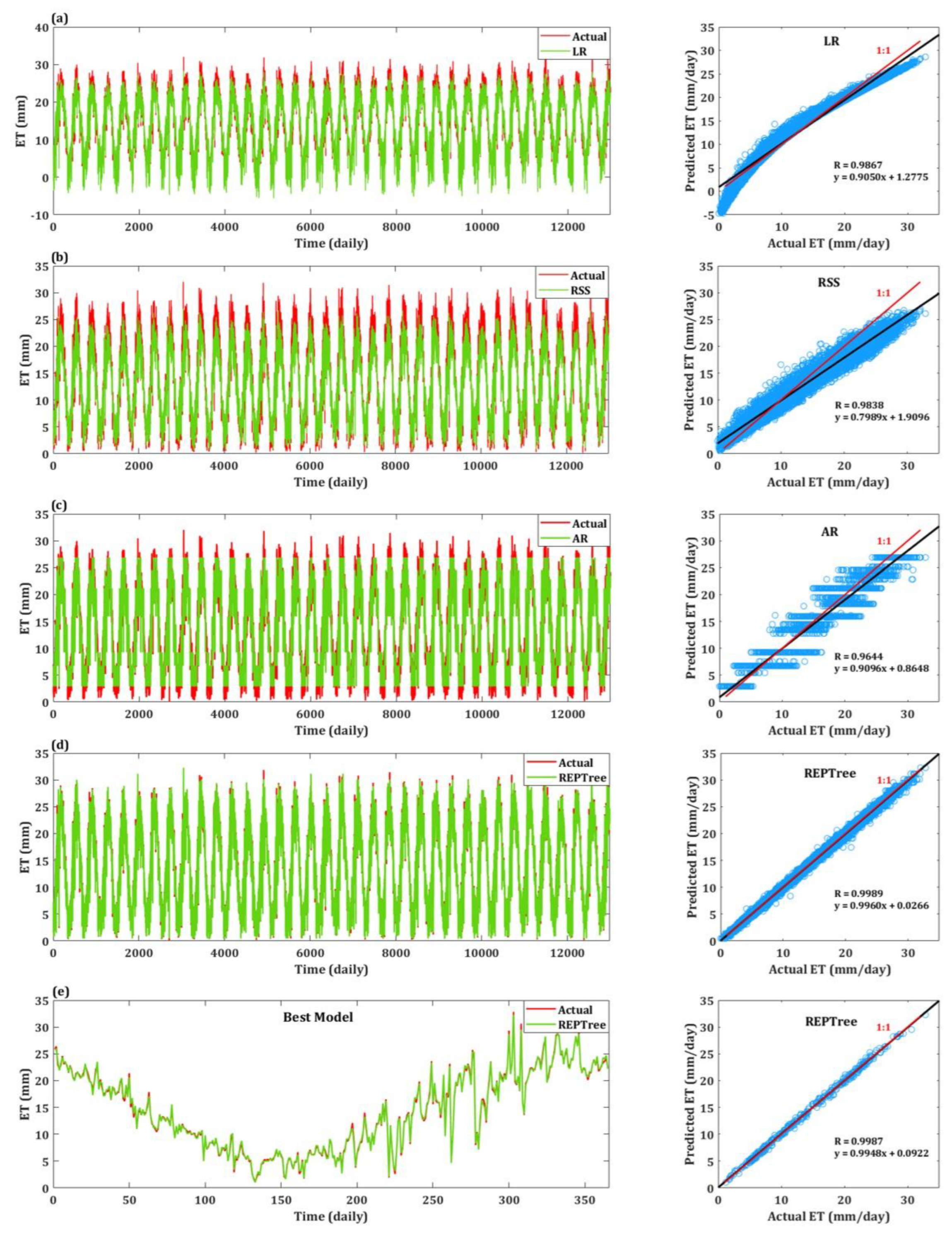
As seen in Figure 6, time-series plots representing observed and modeled ET_o data and scattered plots showing the whole testing dataset of observed vs. estimated ET_o values were developed for the LR, RSS, AR, and REPTree models throughout the testing phase. The regression line, as shown in the scatter plot, was used for the assessment of model performance. The R² value was assessed to be 0.9867 for the LR model, 0.9838 for the RSS model, 0.9644 for the AR model, and 0.9989 for the REPTree model. All the models (except for REPTree) underestimated the ET_o prediction, as the models were observed located below the best-fit 1:1 line. Nevertheless, the REPtree model was observed located nearest to the best-fit 1:1 line. In coherence to the inference made in the previous section, the model REPTree here, too, was implied as the best model for estimating the daily ET_o for the present study site. For this, an additional sample time-series and scatter plot is shown in Figure 6e, indicating a higher correlation (similar to the entire time-series and scatter plot of REPTree) for the most recent study year.

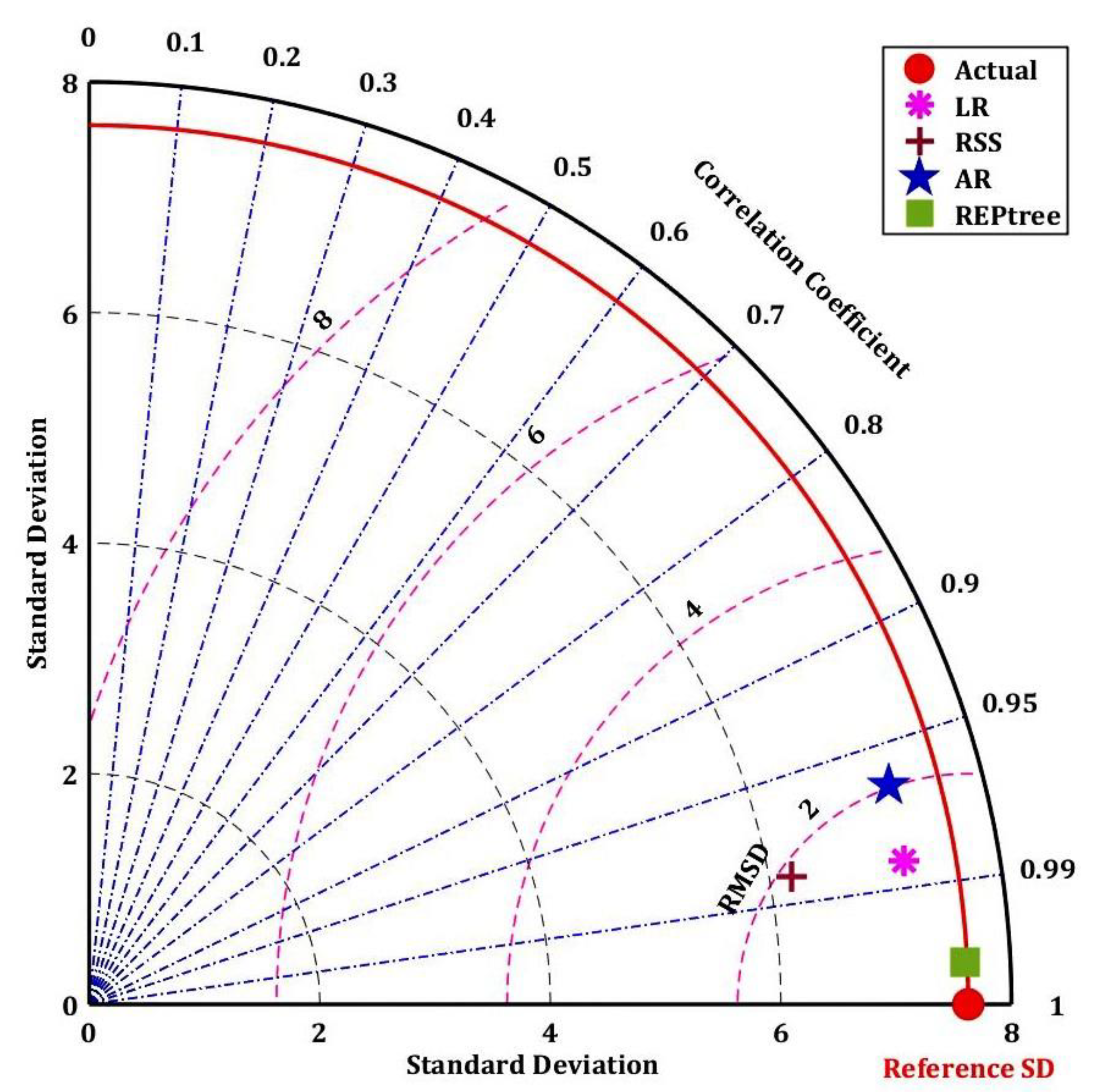
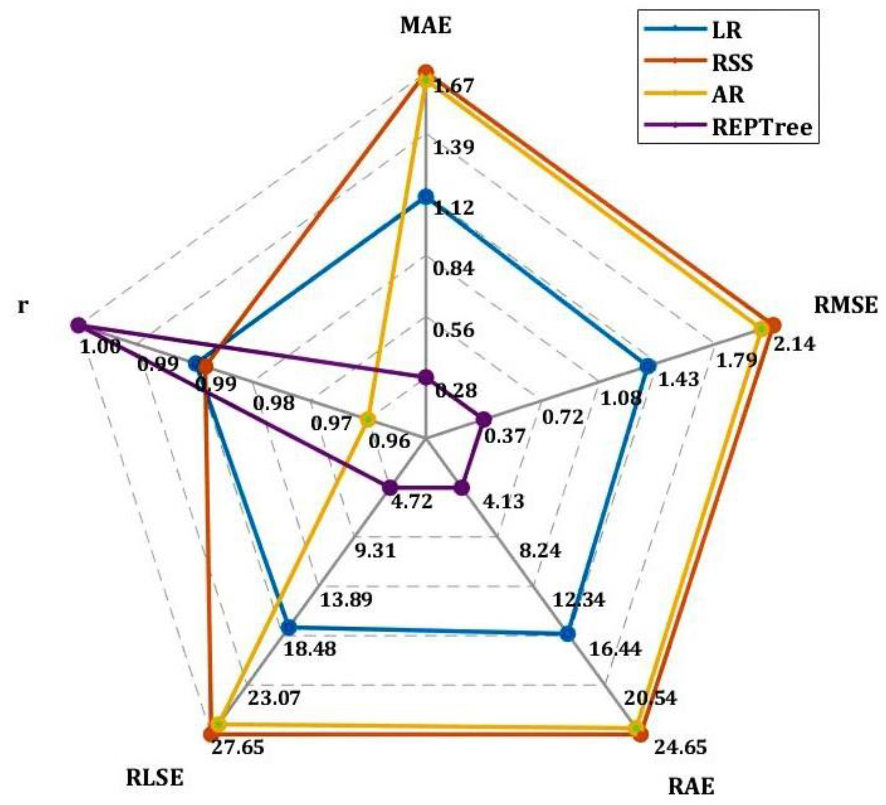
A radar chart for demonstrating the best performance indicators (i.e., best-calculated values for MAE, RMSE, RAE, RRSE, and r) of LR, RSS, AR, and REPTree models observed during the testing phase is shown in Figure 7. This allowed for better diagnostic assessment of the efficiency of all models. Results indicated that the model REPTree has lower values for MAE, RMSE, RAE, and RRSE and higher values for r as compared to the other models. It can be inferred that performance-wise, the model REPTree outperformed other models. Furthermore, a comparative analysis was conducted between the aforesaid models using the Taylor diagram, as shown in Figure 8. This exercise was based on the magnitudes of standard deviation (SD), r, and RMSE obtained during the testing phase. Findings indicated that the model REPTree was found to be the closest to the observed location, while the model AR was found to be the furthest. Given this evidence, the present study summarized that the model AR is the worst-performing model, whereas the model REPTree is the best-performing model among the selected models.

5. Discussion

The present study attempted to test various ML algorithms and their accuracy in predicting the ET_o variable. Considering the findings of this study, it can be broadly inferred that all the four ML algorithm-based models, i.e., LR, RSS, AR, and REPTree, developed in this study more or less demonstrated their predictive capabilities in estimating ET_o. Through a comparative analysis, this study suggested REPTree as the most suitable model for advancing further investigation in the study area. The model REPTree was observed to outclass other models based on satisfying all criteria for performance indicators, as the indicators obtained the most-appropriate values (lowest for MAE, RMSE, RAE, and RRSE and highest for r). These results were further supported by the findings from time-series and scattered plots (refer to Figure 6) as well as from radar chart (Figure 7) and Taylor diagram (Figure 8) developed for comparing the four ML algorithms. They comprehensively indicated REPTree as the best model for the prediction of ET_o, followed by LR, while the model AR was comparatively found to be the worst-performing model for the present study site.

Amidst the ongoing research on estimating reference evapotranspiration, it is imperative to highlight here that the point of novelty for this research lies in using the model REPTree for estimating and predicting ET_o. In addition, the present study determined REPTree as the most suitable model among the models developed to estimate the same. Both these inferences are against the ongoing trend, where researchers have primarily focused on estimating ET_o using other machine learning algorithms. Many studies in recent times have been conducted to estimate hydrologic variables such as pan evaporation, evapotranspiration, etc., from across the globe using ML algorithms. Sattari et al. [52] successfully evaluated the deep learning-based gated recurrent units (GRUs) and tree-based models for estimating ET_o as a case study in Turkey. They found GRUs as the best- and REPTree as the worst-performing model. Kushwaha et al. [53] examined the performance of the four meta-heuristic algorithms, i.e., support vector machine (SVM), random tree (RT), REPTree, and RSS, for simulating daily pan evaporation at two different locations in north India and observed the greater suitability of the model SVM for prediction compared to the others. Nhu et al. [54] predicted the daily water level of Zrebar Lake in Iran using M5P, random forest (RF), random tree (RT), and REPTree algorithms, wherein their results indicated a good prediction capability for all the developed models other than REPTree. Furthermore, if the literature focusing ET_o estimation using ML algorithms is only considered, no recent studies are found to employ the model REPTree. For example, Salam and Islam [55] evaluated the potential of RT, bagging, and RS ensemble learning algorithms for ET_o prediction in Bangladesh. In that, their study found the model RT to outperform other models while estimating daily ET_o. Tikhamarine et al. [56] explored the potential of support vector regression (SVR) integrated with grey wolf optimizer (SVR-GWO) for ET_o estimation in the north of Algeria and concluded its suitability in the study stations. Kisi et al. [57] developed a radial-basis M5 model tree (RM5Tree) for ET_o prediction in Turkey and evaluated it better than the traditional M5 model tree. Bai et al. [58] evaluated four ensemble ET models (EEMs) that use different ML classifiers such as K-nearest neighbors, RF, SVM, and multi-layer perception neural network (MLP). Their study found that ML-based EEMs outperformed individual ET and conventional EEMs. Granata [20] assessed the M5P tree, bagging, RF, and SVR for how precise an ET_o prediction could be obtained in central Florida by developing models in a varying combination of influencing variables. Mehdizadeh et al. [9] successfully evaluated gene expression programming (GEP), SVM, and multivariate adaptive regression splines (MARS) in estimating ET_o in Iran. Their results shown that the MARS had the best performance in the weather-data-based scenarios. Ferreira et al. [10] estimated daily ET_o in Brazil using ANN and SVM. They found that the ANN and SVM models outperformed the empirical equations studied. Fan et al. [19] successfully evaluated random forest (RF), M5Tree, gradient boosting decision tree (GBDT), and extreme gradient boosting (XGBoost) for estimating daily ET_o in China. According to the results, the ELM and SVM models achieved the best combination of prediction accuracy and stability. The XGBoost and GBDT models performed similarly to the SVM and ELM models in terms of accuracy and stability but with significantly lower computation time. Bellido-Jiménez et al. [59] successfully evaluated MLP, generalized regression neural network (GRNN), extreme learning machine (ELM), SVM, RF, and XGBoost for estimating daily ET_o in Spain. Their findings revealed that GRNN and ELM had the lowest computation time, while MLP and ELM were generally the models with the better performances. In general, all the aforementioned studies jointly concluded through their various model assessments that, other than REPTree, the entire presently developed model in this study was observed to be one of the suitable models among many machine-learning-algorithm-based models for estimating hydrologic variables, especially the ET_o.

To summarize, the present study finds its significance in ascertaining studies related to coupling hydrological investigations with climate change vulnerabilities in view of employing the REPTree model. Given the rapid land-use transformations, especially the agricultural land cover over the Earth, alongside aggravating extreme climatic events such as recurring floods [60,61] immediately followed by chronic droughts [62,63], the 21st century’s climatological research demands improved understanding of various hydrologic variables, such as for the ET_o investigated in the present study. Hence, knowledge of ML algorithms becomes paramount, especially when applying certain algorithms; for example, REPTree is limited while estimating ET_o. Such a study allows estimating the future magnitudes, thereby informing the concerned authorities and administrators to orient their policymaking towards more specific climate-resilient pathways.

6. Conclusions

This research verifies the ability of different techniques of machine learning, such as linear regression (LR), random subspace (RSS), additive regression (AR), and reduced error pruning tree (REPTree) models, to estimate the long-series daily reference evapotranspiration (ET_o) for four sites in Egypt (Al Buhayrah, Alexandria, Ismailiyah, and Minufiyah governorates). In order to achieve this, daily climate data variables (including minimum and maximum temperatures, humidity, wind speed, vapor pressure deficit, and solar radiation) for the studied regions over 36 years from 1979 to 2014 were collected from the National Centers for Environmental Prediction (NCEP) Climate Forecast System Reanalysis (CFSR). In addition, the best subset regression analysis was used to determine the best input combinations of meteorological parameters for calculating the ET_o. Sensitivity analysis was carried out and included all input variables in determining the most influential input variables to predict the ET_o with greater accuracy. The following findings were obtained:

-

The results showed that the best input combination for the ET_o model was determined as four input combinations (T_max/T_min/RH/SR) with high R² (0.967) and high Adj-R² (0.967) and MSE of 1.727;

-

The most sensitive input variables to predict the ET_o with greater accuracy were T_max, T_min, and SR;

-

The REPTree model generated the best results with the highest value for r (0.99) and the lowest values for MAE (0.21), RMSE (0.28), RAE (3.45%), and RRSE (4.01%) during the training phase; it also generated the highest value for r (0.99) and the lowest values for MAE (0.28), RMSE (0.37), RAE (4.13%), and RRSE during the testing phase (4.72%);

-

The AR model generated the worst results with R = 0.9595, MAE = 1.5914, RMSE = 1.9876, RAE = 26.25%, and RRSE = 28.22% during the training phase.

The study found that all four models demonstrated their predictive capabilities, with REPTree emerging as the most suitable model for further investigation. This conclusion is significant, as it diverges from the current trend of using other machine learning algorithms to estimate ET_o. The study’s novelty lies in using REPTree to estimate and predict ET_o, as this algorithm has not been commonly used for this purpose. This finding is important given the urgent need to better understand hydrological variables in light of climate change and land-use transformations. The study underscores the importance of machine learning algorithms in predicting ET_o and their potential for estimating future magnitudes to guide climate-resilient policymaking. The study’s results have broader implications beyond ET_o prediction, as machine learning algorithms have been increasingly employed in hydrologic research. The study contributes to the growing literature on using machine learning algorithms to estimate hydrologic variables such as evapotranspiration, pan evaporation, and water levels. The study’s findings suggest that researchers should consider using REPTree rather than other commonly used algorithms for ET_o prediction. In summary, this study highlights the significance of using REPTree in hydrologic research and its potential for predicting ET_o. The study’s results underscore the importance of machine learning algorithms in guiding climate-resilient policymaking in the face of ongoing climate change and land-use transformations. This research could be useful for managing the water resources in the study area.

References

1. Allen, R.G.; Pereira, L.S.; Raes, D.; Smith, M. Crop Evapotranspiration-Guidelines for Computing Crop Water Requirements-Fao Irrigation and Drainage Paper 56; FAO: Rome, Italy, 1998; Volume 300, p. D05109. Available online: http://www.climasouth.eu/sites/default/files/FAO%2056.pdf (accessed on 1 October 2022).
2. Dhillon, R.; Rojo, F.; Upadhyaya, S.K.; Roach, J.; Coates, R.; Delwiche, M. Prediction of plant water status in almond and walnut trees using a continuous leaf monitoring system. Precis. Agric. 2019, 20, 723–745. [Google Scholar] [CrossRef]
3. Sharma, S.; Regulwar, D.G. Prediction of evapotranspiration by artificial neural network and conventional methods. Int. J. Eng. Res. 2016, 5, 184–187. [Google Scholar]
4. Nouri, H.; Beecham, S.; Kazemi, F.; Hassanli, A.M.; Anderson, S. Remote sensing techniques for predicting evapotranspiration from mixed vegetated surfaces. Hydrol. Earth Syst. Sci. Discuss. 2013, 10, 3897–3925. [Google Scholar] [CrossRef]
5. Lu, G.; Wu, Z.; He, H. Hydrological Cycle and Quantity Forecast; Science Press: Beijing, China, 2010. (In Chinese) [Google Scholar]
6. Jun-Fang, Z.H.A.O.; Jian-Ping, G.U.O.; Zhang, Y.H.; Jing-Wen, X.U. Advances in research of impacts of climate change on agriculture. Chin. J. Agrometeorol. 2010, 31, 200. [Google Scholar]
7. Raza, A.; Hu, Y.; Shoaib, M.; Abd Elnabi, M.K.; Zubair, M.; Nauman, M.; Syed, N.R. A Systematic Review on Estimation of Reference Evapotranspiration under Prisma Guidelines. Pol. J. Environ. Stud. 2021, 30, 5413–5422. [Google Scholar] [CrossRef]
8. Raza, A.; Shoaib, M.; Baig, M.A.I.; Ahmad, S.; Khan, M.M.; Ullah, M.K.; Hashim, S. Comparative study of powerful predictive modeling techniques for modeling monthly reference evapotranspiration in various climatic regions. Fresenius Environ. Bull. 2021, 30, 7490–7513. [Google Scholar]
9. Mehdizadeh, S.; Behmanesh, J.; Khalili, K. Using MARS, SVM, GEP and empirical equations for estimation of monthly mean reference evapotranspiration. Comput. Electron. Agric. 2017, 139, 103–114. [Google Scholar] [CrossRef]
10. Ferreira, L.B.; da Cunha, F.F. New approach to estimate daily reference evapotranspiration based on hourly temperature and relative humidity using machine learning and deep learning. Agric. Water Manag. 2020, 234, 106113. [Google Scholar] [CrossRef]
11. Guo, X.; Sun, X.; Ma, J. Prediction of daily crop reference evapotranspiration (ETo) values through a least-squares support vector machine model. Hydrol. Res. 2011, 42, 268–274. [Google Scholar] [CrossRef]
12. Traore, S.; Luo, Y.; Fipps, G. Deployment of artificial neural network for short-term forecasting of evapotranspiration using public weather forecast restricted messages. Agric. Water Manag. 2016, 163, 363–379. [Google Scholar] [CrossRef]
13. Valipour, M.; Gholami Sefidkouhi, M.A.; Raeini-Sarjaz, M.; Guzman, S.M. A hybrid data-driven machine learning technique for evapotranspiration modeling in various climates. Atmosphere 2019, 10, 311. [Google Scholar] [CrossRef] [Green Version]
14. Mattar, M.A. Using gene expression programming in monthly reference evapotranspiration modeling: A case study in Egypt. Agric. Water Manag. 2018, 198, 28–38. [Google Scholar] [CrossRef]
15. Gocic, M.; Petković, D.; Shamshirband, S.; Kamsin, A. Comparative analysis of reference evapotranspiration equations modelling by extreme learning machine. Comput. Electron. Agric. 2016, 127, 56–63. [Google Scholar] [CrossRef]
16. Abdullah, S.S.; Malek, M.A.; Abdullah, N.S.; Kisi, O.; Yap, K.S. Extreme learning machines: A new approach for prediction of reference evapotranspiration. J. Hydrol. 2015, 527, 184–195. [Google Scholar] [CrossRef]
17. Raza, A.; Shoaib, M.; Faiz, M.A.; Baig, F.; Khan, M.M.; Ullah, M.K.; Zubair, M. Comparative assessment of reference evapotranspiration estimation using conventional method and machine learning algorithms in four climatic regions. Pure Appl. Geophys. 2020, 177, 4479–4508. [Google Scholar] [CrossRef]
18. Raza, A.; Shoaib, M.; Khan, A.; Baig, F.; Faiz, M.A.; Khan, M.M. Application of non-conventional soft computing approaches for estimation of reference evapotranspiration in various climatic regions. Theor. Appl. Climatol. 2020, 139, 1459–1477. [Google Scholar] [CrossRef]
19. Fan, J.; Yue, W.; Wu, L.; Zhang, F.; Cai, H.; Wang, X.; Lu, X.; Xiang, Y. Evaluation of SVM, ELM and four tree-based ensemble models for predicting daily reference evapotranspiration using limited meteorological data in different climates of China. Agric. For. Meteorol. 2018, 263, 225–241. [Google Scholar] [CrossRef]
20. Granata, F. Evapotranspiration evaluation models based on machine learning algorithms—A comparative study. Agric. Water Manag. 2019, 217, 303–315. [Google Scholar] [CrossRef]
21. Elbeltagi, A.; Raza, A.; Hu, Y.; Al-Ansari, N.; Kushwaha, N.L.; Srivastava, A.; Zubair, M. Data intelligence and hybrid metaheuristic algorithms-based estimation of reference evapotranspiration. Appl. Water Sci. 2022, 12, 152. [Google Scholar] [CrossRef]
22. Feng, Y.; Cui, N.; Gong, D.; Zhang, Q.; Zhao, L. Evaluation of random forests and generalized regression neural networks for daily reference evapotranspiration modelling. Agric. Water Manag. 2017, 193, 163–173. [Google Scholar] [CrossRef]
23. Feng, Y.; Peng, Y.; Cui, N.; Gong, D.; Zhang, K. Modeling reference evapotranspiration using extreme learning machine and generalized regression neural network only with temperature data. Comput. Electron. Agric. 2017, 136, 71–78. [Google Scholar] [CrossRef]
24. Fang, W.; Huang, S.; Huang, Q.; Huang, G.; Meng, E.; Luan, J. Reference evapotranspiration forecasting based on local meteorological and global climate information screened by partial mutual information. J. Hydrol. 2018, 561, 764–779. [Google Scholar] [CrossRef]
25. Saggi, M.K.; Jain, S. Reference evapotranspiration estimation and modeling of the Punjab Northern India using deep learning. Comput. Electron. Agric. 2019, 156, 387–398. [Google Scholar] [CrossRef]
26. Huang, G.; Wu, L.; Ma, X.; Zhang, W.; Fan, J.; Yu, X.; Zeng, W.; Zhou, H. Evaluation of CatBoost method for prediction of reference evapotranspiration in humid regions. J. Hydrol. 2019, 574, 1029–1041. [Google Scholar] [CrossRef]
27. Torres, A.F.; Walker, W.R.; McKee, M. Forecasting daily potential evapotranspiration using machine learning and limited climatic data. Agric. Water Manag. 2011, 98, 553–562. [Google Scholar] [CrossRef]
28. Tang, D.; Feng, Y.; Gong, D.; Hao, W.; Cui, N. Evaluation of artificial intelligence models for actual crop evapotranspiration modeling in mulched and non-mulched maize croplands. Comput. Electron. Agric. 2018, 152, 375–384. [Google Scholar] [CrossRef]
29. Walls, S.; Binns, A.D.; Levison, J.; MacRitchie, S. Prediction of actual evapotranspiration by artificial neural network models using data from a Bowen ratio energy balance station. Neural Comput. Appl. 2020, 32, 14001–14018. [Google Scholar] [CrossRef]
30. Nourani, V.; Elkiran, G.; Abdullahi, J. Multi-station artificial intelligence based ensemble modeling of reference evapotranspiration using pan evaporation measurements. J. Hydrol. 2019, 577, 123958. [Google Scholar] [CrossRef]
31. Tabari, H.; Martinez, C.; Ezani, A.; Hosseinzadeh Talaee, P. Applicability of support vector machines and adaptive neurofuzzy inference system for modeling potato crop evapotranspiration. Irrig. Sci. 2013, 31, 575–588. [Google Scholar] [CrossRef]
32. CAPMAS (Central Agency for Public Mobilization and Statistics). Egypt in Figures: Population. 2022. Available online: https://www.capmas.gov.eg/Pages/StaticPages.aspx?page_id=5035# (accessed on 15 October 2022).
33. Ayaz, A.; Rajesh, M.; Singh, S.K.; Rehana, S. Estimation of reference evapotranspiration using machine learning models with limited data. AIMS Geosci. 2021, 7, 268–290. [Google Scholar] [CrossRef]
34. Ho, T.K. The random subspace method for constructing decision forests. IEEE Trans. Pattern Anal. Mach. Intell. 1998, 20, 832–844. [Google Scholar]
35. Yaman, M.A.; Subasi, A.; Rattay, F. Comparison of random subspace and voting ensemble machine learning methods for face recognition. Symmetry 2018, 10, 651. [Google Scholar] [CrossRef] [Green Version]
36. Skurichina, M.; Duin, R.P. Bagging, boosting and the random subspace method for linear classifiers. Pattern Anal. Appl. 2002, 5, 121–135. [Google Scholar] [CrossRef]
37. Xia, C.; Pan, Z.; Polden, J.; Li, H.; Xu, Y.; Chen, S. Modelling and prediction of surface roughness in wire arc additive manufacturing using machine learning. J. Intell. Manuf. 2022, 33, 1467–1482. [Google Scholar] [CrossRef]
38. Ravikumar, P.; Lafferty, J.; Liu, H.; Wasserman, L. Sparse additive models. J. R. Stat. Soc. Ser. B 2009, 71, 1009–1030. [Google Scholar] [CrossRef]
39. Hastie, T.; Tibshirani, R. Generalized Additive Models. Stat. Sci. 1986, 6, 15–51. [Google Scholar] [CrossRef]
40. Laanaya, F.; St-Hilaire, A.; Gloaguen, E. Water temperature modelling: Comparison between the generalized additive model, logistic, residuals regression and linear regression models. Hydrol. Sci. J. 2017, 62, 1078–1093. [Google Scholar] [CrossRef]
41. Fu, J.C.; Huang, H.Y.; Jang, J.H.; Huang, P.H. River Stage Forecasting Using Multiple Additive Regression Trees. Water Resour. Manag. 2019, 33, 4491–4507. [Google Scholar] [CrossRef]
42. Senthil Kumar, A.R.; Ojha, C.S.P.; Goyal, M.K.; Singh, R.D.; Swamee, P.K. Modeling of Suspended Sediment Concentration at Kasol in India Using ANN, Fuzzy Logic, and Decision Tree Algorithms. J. Hydrol. Eng. 2012, 17, 394–404. [Google Scholar] [CrossRef]
43. Witten, I.H.; Frank, E. Data mining: Practical machine learning tools and techniques with Java implementations. Acm Sigmod Record 2002, 31, 76–77. [Google Scholar] [CrossRef]
44. Quinlan, J. Simplifying decision trees. Int. J. Man-Mach. Stud. 1987, 27, 221–234. [Google Scholar] [CrossRef] [Green Version]
45. Bharti, B.; Pandey, A.; Tripathi, S.K.; Kumar, D. Modelling of runoff and sediment yield using ANN, LS-SVR, REPTree and M5 models. Hydrol. Res. 2017, 48, 1489–1507. [Google Scholar] [CrossRef] [Green Version]
46. Breiman, L. Bagging predictors. Mach. Learn. 1996, 24, 123–140. [Google Scholar] [CrossRef] [Green Version]
47. Joseph, K.S.; Ravichandran, T. A comparative evaluation of software effort estimation using REPTree and K* in handling with missing values. Aust. J. Basic Appl. Sci. 2012, 6, 312–317. [Google Scholar]
48. Pérez-Domínguez, L.; Garg, H.; Luviano-Cruz, D.; García Alcaraz, J.L. Estimation of Linear Regression with the Dimensional Analysis Method. Mathematics 2022, 10, 1645. [Google Scholar] [CrossRef]
49. Hothorn, T.; Bretz, F.; Westfall, P. Simultaneous inference in general parametric models. Biom. J. J. Math. Methods Biosci. 2008, 50, 346–363. [Google Scholar] [CrossRef] [PubMed] [Green Version]
50. Liu, M.; Hu, S.; Ge, Y.; Heuvelink, G.B.; Ren, Z.; Huang, X. Using multiple linear regression and random forests to identify spatial poverty determinants in rural China. Spat. Stat. 2020, 42, 100461. [Google Scholar] [CrossRef]
51. Park, J.Y.; Phillips, P.C. Statistical inference in regressions with integrated processes: Part 2. Econom. Theory 1989, 5, 95–131. [Google Scholar] [CrossRef] [Green Version]
52. Sattari, M.T.; Apaydin, H.; Shamshirband, S. Performance evaluation of deep learning-based gated recurrent units (GRUs) and tree-based models for estimating ETo by using limited meteorological variables. Mathematics 2020, 8, 972. [Google Scholar] [CrossRef]
53. Kushwaha, N.L.; Rajput, J.; Elbeltagi, A.; Elnaggar, A.Y.; Sena, D.R.; Vishwakarma, D.K.; Mani, I.; Hussein, E.E. Data intelligence model and meta-heuristic algorithms-based pan evaporation modelling in two different agro-climatic zones: A case study from northern India. Atmosphere 2021, 12, 1654. [Google Scholar] [CrossRef]
54. Nhu, V.H.; Shahabi, H.; Nohani, E.; Shirzadi, A.; Al-Ansari, N.; Bahrami, S.; Miraki, S.; Geertsema, M.; Nguyen, H. Daily water level prediction of Zrebar Lake (Iran): A comparison between M5P, random forest, random tree and reduced error pruning trees algorithms. ISPRS Int. J. Geo-Inf. 2020, 9, 479. [Google Scholar] [CrossRef]
55. Salam, R.; Islam, A.R.M.T. Potential of RT, Bagging and RS ensemble learning algorithms for reference evapotranspiration prediction using climatic data-limited humid region in Bangladesh. J. Hydrol. 2020, 590, 125241. [Google Scholar] [CrossRef]
56. Tikhamarine, Y.; Malik, A.; Souag-Gamane, D.; Kisi, O. Artificial intelligence models versus empirical equations for modeling monthly reference evapotranspiration. Environ. Sci. Pollut. Res. 2020, 27, 30001–30019. [Google Scholar] [CrossRef] [PubMed]
57. Kisi, O.; Keshtegar, B.; Zounemat-Kermani, M.; Heddam, S.; Trung, N.T. Modeling reference evapotranspiration using a novel regression-based method: Radial basis M5 model tree. Theor. Appl. Climatol. 2021, 145, 639–659. [Google Scholar] [CrossRef]
58. Bai, Y.; Zhang, S.; Bhattarai, N.; Mallick, K.; Liu, Q.; Tang, L.; Im, J.; Guo, L.; Zhang, J. On the use of machine learning based ensemble approaches to improve evapotranspiration estimates from croplands across a wide environmental gradient. Agric. For. Meteorol. 2021, 298, 108308. [Google Scholar] [CrossRef]
59. Bellido-Jiménez, J.A.; Estévez, J.; García-Marín, A.P. New machine learning approaches to improve reference evapotranspiration estimates using intra-daily temperature-based variables in a semi-arid region of Spain. Agric. Water Manag. 2021, 245, 106558. [Google Scholar] [CrossRef]
60. Arnell, N.W.; Gosling, S.N. The impacts of climate change on river flood risk at the global scale. Clim. Change 2016, 134, 387–401. [Google Scholar] [CrossRef] [Green Version]
61. Khadke, L.; Pattnaik, S. Impact of initial conditions and cloud parameterization on the heavy rainfall event of Kerala (2018). Model. Earth Syst. Environ. 2021, 7, 2809–2822. [Google Scholar] [CrossRef]
62. Meza, I.; Siebert, S.; Döll, P.; Kusche, J.; Herbert, C.; Eyshi Rezaei, E.; Nouri, H.; Gerdener, H.; Popat, E.; Frischen, J.; et al. Global-scale drought risk assessment for agricultural systems. Nat. Hazards Earth Syst. Sci. 2020, 20, 695–712. [Google Scholar] [CrossRef] [Green Version]
63. Sazib, N.; Mladenova, I.; Bolten, J. Leveraging the google earth engine for drought assessment using global soil moisture data. Remote Sens. 2018, 10, 1265. [Google Scholar] [CrossRef] [PubMed] [Green Version]
Figure 1. Location of the study area (Al Buhayrah, Alexandria, Ismailiyah, and Minufiyah governorates) in Egypt.
Water 15 01149 g001
Figure 2. Demonstration of time series of each input variable used for developing ML models for simulating the evapotranspiration process.
Water 15 01149 g002
Figure 3. Flowchart of ETo estimation methodology in the study area.
Water 15 01149 g003
Figure 4. Inter-correlation matrix of selected climatic variables for ETo.
Water 15 01149 g004
Figure 5. Standardized coefficients of input variable for sensitivity analysis for ETo.
Water 15 01149 g005
Figure 6. Time-series plots (left) represent observed and modeled ETo data, and scattered plots (right) represent the entire testing dataset of observed versus estimated ETo values during the testing phase for the models ((a) LR, (b) RSS, (c) AR, (d) and (e) RETree).
Water 15 01149 g006
Figure 7. Radar chart displaying the best performance indicators of ML models.
Water 15 01149 g007
Figure 8. Taylor diagrams of models during the testing phase.
Water 15 01149 g008