Article

Cross-Correlation Analysis of the Stability of Heterogeneous Slopes

1
School of Earth Sciences and Engineering, Hohai University, Nanjing 211100, China
2
Department of Hydrology and Atmospheric Sciences, University of Arizona, Tucson, AZ 85721, USA
*
Author to whom correspondence should be addressed.
Water 2023, 15(6), 1050; https://doi.org/10.3390/w15061050
Submission received: 14 February 2023 / Revised: 6 March 2023 / Accepted: 7 March 2023 / Published: 9 March 2023

Abstract

:
Geologic material properties of hillslopes are inherently heterogeneous, with complex layering structures due to geological deposition processes. Lacking detailed sampling of the properties’ spatial distribution has led to the stochastic representation of the properties to address uncertainty in the hillslope stability evaluation. This study treats the spatial distributions of the shear strength parameters, the cohesion (c), and the internal friction angle (φ), in a synthetic two-dimensional slope as stochastic random fields characterized by their means, variances, and correlation scales. This study then evaluates the cross-correlation between these parameters and the factor of safety (FS) using unconditional Monte Carlo simulation (MCS). Different from classical sensitivity analyses, the cross-correlation analysis of FS and the stochastic parameter fields stresses the importance of the orientation of the large-scale geological layering, the correlation between the geological media’s cohesion, and the internal friction angle at the local scale on the probability and uncertainty of failure of the heterogeneous hillslope. The analysis further guides the field sampling strategy to reduce uncertainty in the slope stability analysis due to unknown heterogeneity. More importantly, it suggests the location of stability reinforcement measures. The results of this study provide cost-effective tools for geoengineers to deal with field slope stability analysis under uncertainty.

1. Introduction

Shear strength parameters (cohesion (c) and internal friction angle (φ)) are the critical parameters for evaluating slope stability. These parameters exhibit spatial variability at different scales due to complex geological processes [1,2,3]. Many previous studies have concluded that the spatial variability of geotechnical properties is vital in slope stability evaluations [4,5,6]. For example, Qi et al. [7] investigated the effect of the spatial variability of shear strength parameters on a two-dimensional slope’s critical slip surface distribution. Griffiths et al. [8] and Jiang et al. [9] suggested that ignoring the spatial variability of the shear strength parameters would lead to an underestimation of the probability of slope failure when the coefficient of variation of the shear strength parameters was significant. The slope stability evaluated using the mean value of the parameter could be misleading. Cho [10] emphasized the importance of the spatial variability of soil mechanics’ parameters in evaluating failure probability. Additionally, the effect of the spatial variability of soil properties is crucial when the slope risk assessment is over large areas due to both the variability and lack of measurements [11,12]. Based on genetic algorithms and machine learning, Miao et al. [13,14] performed displacement prediction and landslide susceptibility mapping over a large area and evaluated its uncertainty.
In recent years, geostatistical random field theory has been used to describe the heterogeneity of parameters, using its mean, variance, and correlation scales to describe the most probable values, variability, and spatial structure of the parameter fields [15]. The heterogeneous parameter field is statistically isotropic when the horizontal correlation scale is equal to the vertical correlation scale. The field is statistically anisotropic when the horizontal correlation scale is different from the vertical correlation scale.
Combining random fields and Monte Carlo simulations (MCS), one can conduct a cross-correlation analysis of heterogeneous shear-strength parameters and slope stability. Cross-correlation analysis is a method that reveals the spatial relationship between parameters and processes, considering the variance and spatial structure of the parameters. Recently, Cai et al. [16] proposed an effective sampling strategy in slope stability evaluation based on the cross-correlation analysis of shear strength parameters and the factor of safety (FS), defined as the ratio of the slope’s absolute strength to the actual applied load. Cross-correlation analysis is widely used in many fields, such as underground engineering and groundwater science. Using cross-correlation analysis, Gao et al. [17] investigated the spatial relationship between the rock parameters of the unlined rock caverns and the displacement at a location of interest. Mao et al. [18] studied the relationship between observed heads and hydraulic properties at different times and locations of unconfined aquifers during pumping tests. Sun et al. [19] proposed a temporal sampling strategy based on the cross-correlation analysis of hydraulic parameters and observed hydraulic heads.
Most current studies have investigated the effect of the coefficient of variation of parameters on slope stability with statistical isotropic media. However, due to sedimentation processes, geotechnical material often displays a layered structure [7,20,21,22,23]. The failure types of slopes with layered structures are generally translational slides, mudslides, and creep-fatigue [24,25,26]. That is, the correlation scales in different directions of the parameters are different, which leads to the fact that parameter fields with statistical anisotropy are standard. Moreover, Cai et al. [27] developed an analytical approach for the reliability analysis of infinite slope stability in the presence of spatially variable shear-strength parameters. They concluded that the pf increases when the correlation between c and tanφ increases. Griffiths et al. [8] and Jiang et al. [9] obtained similar conclusions by studying two-dimensional heterogeneous slopes using the random finite element method. The correlation between c and tanφ significantly influences the probability of slope failure. However, the influence of the correlation between c and tanφ on slope stability considering parameter statistical anisotropy has not been comprehensively studied. Likewise, studies have compared the effect of the conditional random field with the unconditional random field on slope stability analysis using MCS with the finite element method. They concluded that conditional random field simulations could address the reduction in uncertainty due to conditioning with sampled parameters in evaluating slope stability [28,29,30,31]. Nonetheless, these studies have not addressed the vital issue of reducing uncertainty by selecting sampling locations. This issue (where to sample and how many sampling locations) to reduce the uncertainty is critical since only a limited number of samples is available in field situations.
This paper investigates the effect of statistical anisotropy of shear strength parameters on slope stability. We first introduce the influence of the correlation scale on the parameter distribution and the method of cross-correlation analysis between the parameters and FS. Then, we use a two-dimensional slope with statistical isotropy to analyze the cross-correlation between parameters and FS. The comparison of the correlation analysis, sensitivity analysis, and traditional limit equilibrium method comes next. The analyses of the cross-correlations between parameters and FS, and the influences of the correlation scales on slope stability in statistically anisotropic media are investigated. Lastly, using conditional random fields with MCS, we compared the uncertainty in evaluating slope stability for four different sampling schemes to validate the results of the cross-correlation analysis.

2. Methodology

2.1. Random Field Modeling of Heterogeneity

This study adopts the random field theory to describe the heterogeneity of shear strength parameters. The impossibility of obtaining the parameter values at every slope location recommends that we consider the c (or φ) of each position as a random variable. A collection of these random variables of c (or φ) in the entire slope becomes a random field characterized by a joint probability density function with mean, variance, and autocorrelation function, which describes the probability of a parameter value at any slope location. The mean represents the most likely value of the parameter, and the variance represents its average deviation from the actual value (i.e., uncertainty) due to variability and lack of measurements. On the other hand, the autocorrelation function quantifies the parameter’s spatial structure (average spatial distribution of the clusters of the geotechnical properties in the slope).
Suppose the slope has n × n random variables, and i and j = 1,2…, n, a two-dimensional autocorrelation function is represented as follows:
ρ i j = exp 2 x i x j λ x + y i y j λ y
where ρij is the autocorrelation coefficient between the parameter at location (xi, yi) and location (xj, yj), and λx and λy are the horizontal and vertical correlation scales, respectively. Many other forms of the autocorrelation function are available. They all are ensemble statistics (i.e., general knowledge). We, therefore, chose the most simplistic one. This study considers the correlation scales of c and tanφ as the same.
Physically, the correlation scale represents the average dimensions (e.g., length, width, and thickness) of heterogeneity (e.g., layers or stratifications) within the domain [32]. With specified mean, variance, and correlation scales, numerous realizations of parameter distributions can be generated with different random seeds by a spectral representation method [33,34]. In order to avoid negative values while generating the random fields, the natural log-normal distribution of c and tanφ are employed. Figure 1 shows six realizations of the cohesion parameter field with the same mean and variance (μc = 15 kN/m2, σc = 7.5 kN/m2), but with different correlation scales. These fields are called statistically isotropic when the λx is the same as the λy (Figure 1a,b), and statistically anisotropic when the λx is different from the λy (Figure 1c–f). In Figure 1c,d, the correlation scales are 1 m in the vertical direction and 5 m and 10 m in the horizontal direction, respectively. As the λx becomes large, the strong and weak zones extend greatly in the horizontal direction, and the slope shows an apparent horizontal layered structure. Figure 1e,f display the cases where λx = 1 m, λy = 5 m and λx = 1 m, λy =10 m, respectively. The slope exhibits a vertically layered structure as the λy becomes greater than the λx. In this study, we consider different cases as follows. For statistical isotropy: λx = λy = 1 m; for statistical horizontal anisotropy: λy = 1 m, λx = 5 m, 10 m, 20 m, 40 m, 80 m, respectively; for statistical vertical anisotropy: λx = 1 m, λy = 5 m, 10 m, 20 m, 40 m, respectively.

2.2. Slope Stability Analysis

MCS is one of the widely utilized methods to estimate the probability of failure and the reliability of a slope with the general knowledge of the mean, variance, and correlation scales of the geotechnical properties of a hill slope. This study, different from many previous studies, adopts the MCS to investigate the effects of correlation scales on the analysis of the probability of failure and reliability of a slope and guides the sampling scheme to reduce the uncertainty of our estimated probability and reliability.
For this purpose, a two-dimensional synthetic slope model for plane strain analysis (Figure 2) with a slope height H = 10 m and slope inclination α = 26.6° was discretized into 385 elements with 1 m × 1 m in size, and some of them are truncated because of the slope surface. The left and right boundaries of the model are zero horizontal displacements (ux = 0 m), the bottom boundaries are zero horizontal and vertical displacements (ux = 0 m, uy = 0 m), and the slope surface is free displacement. The slope is assumed to be subjected to gravity loads only and consists of elastic–perfectly plastic soils following the Mohr–Coulomb failure criterion. Specifically, the loading stress at each element is the total weight of the element above, and the shear strength of each element follows the Mohr–Coulomb failure criterion. Other complex or advanced constitutive models [35,36,37] or numerical simulation methods [38] could be used with corresponding randomized input parameters. Table 1 lists the statistics of soil mechanical parameters, except for their correlation scales. Subsequently, the corresponding FS for the entire slope was evaluated based on the finite element strength reduction method (SRM) [39,40]. The program for calculating FS in this study is mainly based on the program p64 [40], and the main difference lies in the automatic MCS and the search for the critical strength reduction factor. The SRM has been widely used due to its practicality and reliability. The factor of safety (FS) is defined as the proportion by which c and tanφ must be reduced in order to cause slope failure. The strength reduction based on the Mohr–Coulomb criterion is shown in the following equation [39,40]:
c trial = c S R F
tan φ trial = tan φ S R F
where SRF is the strength reduction factor; ctrial and tanφtrial are the trial shear strength parameters, which decrease with an increase in SRF. Several gradually increasing values of the SRF are tested, and the updated ctrial and tanφtrial are used for elastoplastic analysis. When the algorithm does not converge for 1000 iterations, the slope is considered as having failed in this study. The smallest value of SRF causing failure is then interpreted as the factor of safety FS. For example, the FS of this slope using the mean values (Table 1) as input parameters, considering the slope as homogeneous, is 1.141.
Using this synthetic hill slope model and MCS, we evaluated the probability of slope failure pf and the reliability index β according to the following formula [16]:
p f = N F S < 1 N
β = μ F S 1 σ F S
where N is the number of realizations in MCS; in this study, N = 500 realizations. NFS<1 is the number of realizations whose FS value is less than 1 (i.e., the slope fails). A small value of NFS<1 implies that the probability of failure of the slope is small. In Equation (5), μFS is the mean value and σFS is the standard deviation of FS values of N realizations of MCS. (μFS − 1) represents the slope stability and σFS represents the uncertainty in the evaluating FS. Therefore, the larger β is, the more reliable the estimated FS is and the smaller the probability of slope failure.

2.3. Cross-Correlation Analysis

In the next step, we investigate the sensitivity of a slope’s FS to the parameters’ heterogeneity at every part of the slope. Cross-correlation analysis is the sensitivity analysis of system response cast in a stochastic framework with the consideration of variability (variance) and spatial structure (correlation scales) of the heterogeneous slope (e.g., [18,19]). Specifically, a cross-correlation map represents the most likely relationship between system responses and spatial variability in system properties. This study applies the cross-correlation analysis to examine the relationship between shear strength parameters and slope stability:
ρ F S c x i = 1 N k N F S k μ F S × c x i , k μ c x i σ F S σ c x i
ρ F S tan φ x i = 1 N k N F S k μ F S × tan φ x i , k μ tan φ x i σ F S σ tan φ x i
where x i is the position vector of the parameter considered; ρFSc( x i ) and ρFStanφ( x i ) are the cross-correlations between the cohesion and the internal friction angle at the location x i and FS, respectively. FSk is the FS at the kth realization; c( x i ,k) is the cohesion at the location x i and kth realization; tanφ( x i ,k) is the tangent of the internal friction angle at the location x i and kth realization. Lastly, σc( x i ) is the standard deviation of the cohesion; σtanφ( x i ) is the standard deviation of tanφ.

3. Results of Cross-Correlation Analysis for Statistical Isotropy

This section examines the cross-correlation between FS and two independent variables (cohesion c and the internal friction angle tanφ) with correlation scales of 1 m in both horizontal and vertical directions (statistically isotropic cases). The cross-correlation maps between the shear strength parameters and FS (Figure 3) reveal that ρFSc is positive at the toe and the top of the slope (Figure 3a), suggesting a large c value at these areas leads to the greater FS value of the slope. On the other hand, the interior of the slope areas has a positive correlation between tanφ and FS (Figure 3b). The remaining areas have correlation values close to zero, meaning that shear strength in these areas (i.e., most of the slope surface and the back of the slope.) has little effect on the slope stability.
Comparing Figure 3a,b, we observe that the locations of the positive correlation regions of the two parameters are different. Such a difference implies that the mechanisms of c and tanφ on slope stability are different within the slope. Physically, c is the maximum shear stress a rupture surface can carry when the normal stress is absent. On the other hand, tanφ is the coefficient that converts the normal stress at the rupture surface to frictional force. According to the Mohr–Coulomb yield criterion, the shear strength of a geotechnical material is equal to the sum of c and the normal stress multiplied by tanφ. In the interior of the slope, due to the gravity of the overlying material of the slope, the material in the interior is subjected to high normal stresses, and the coefficient tanφ becomes the key factor transforming the normal stress into the anti-slip force. The larger tanφ is, the greater the anti-slip force under the same normal stress. Therefore, the value of tanφ in the slope’s interior greatly influences the slope stability.
On the other hand, at the toe and top of the slope, the geotechnical mass experiences low normal stress, and the material’s cohesion c dictates the shear strength and influences slope stability. The above discussions should explain the differences in the cross-correlation patterns in Figure 3a,b. For this reason, one must recognize that the impact areas of these two parameters are different when evaluating slope stability.
Comparing the potential sliding surface (the red line in Figure 3) calculated by the limit equilibrium method [41] using the mean values of parameters, we observe that the region of positive correlation partially overlaps the surface. This result demonstrates that the cross-correlation analysis of FS and parameters pinpoint the slope’s critical areas. Moreover, the cross-correlation analysis identifies potential sliding zones in contrast to a single sliding surface obtained by the limit equilibrium method.
The sensitivity analysis results of FS to the cohesion (the sensitivity of FS to c, Jc, Figure 4a) and internal friction angle (the sensitivity of FS to tanφ, Jtanφ, Figure 4b) display similar patterns to those in Figure 3a,b, derived from MCS. The sensitivity analysis of FS to the parameter takes the following steps. First, the parameter at each location is set as the mean value, and the FS of the homogeneous slope is evaluated by the finite element strength-reduction method. Then, we applied a perturbation of the parameter at a spatial location xi, keeping the parameter at the other locations as the mean value. We subsequently evaluated the FS corresponding to this perturbation. The ratio of the change of FS to the perturbation is the sensitivity of FS to the parameter at this position. After calculating the sensitivity at each location, we derived a sensitivity map. The map shows that the sensitivity of FS to c is greater at the foot and top of the slope compared to other regions, and the sensitivity of FS to tanφ is more significant in the interior of the slope. Notice that the sensitivity analysis, based on the perturbation method, aims at the change of FS per change in the given mean value of the parameter, ignoring the variability (variance) and spatial structure (correlation scale) of the parameters [42]. Specifically, the cross-correlation analysis considers many possible slopes with heterogeneous parameter fields with the same mean parameter value but different perturbations and spatial structure patterns. It then summarizes the results statistically. Consequently, the sensitivity analysis results (Figure 4) differ from the cross-correlation analysis (Figure 3), and the cross-correlation analysis is most appropriate for cases where spatial parameter values are unknown (i.e., realistic field situations).

4. Results of Cross-Correlation Analysis for Statistical Anisotropy

4.1. Statistical Horizontal Anisotropy (Horizontal Correlation Scale > Vertical Correlation Scale)

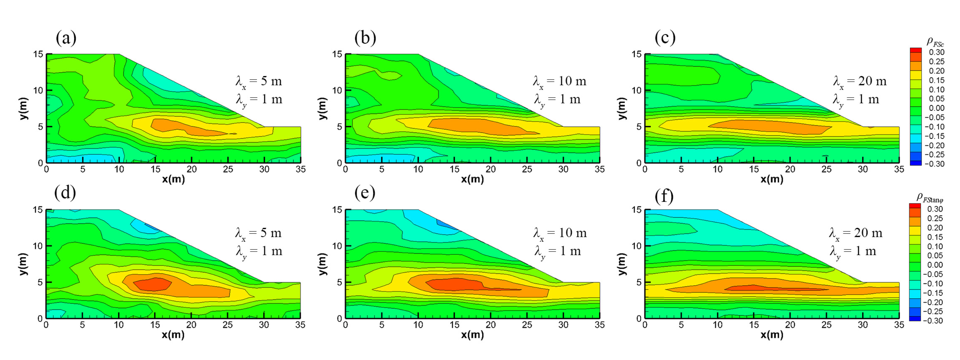
This section investigates the results of the cross-correlation analysis between FS and shear strength parameters (c and tanφ) with different λx values (Figure 5) while λy = 1 m. Figure 5a,c show the cross-correlation maps between FS and c, for λx of c equal to 5, 10, and 20 m, respectively. The cross-correlation maps between FS and tanφ, for λx of tanφ equal to 5, 10, and 20 m are presented in Figure 5d,f, respectively. We observe that the positive areas of ρFSc and ρFStanφ expand as λx increases, but the areas are confined to the areas at the slope toe. Comparing the results to the cross-correlation map of the statistically isotropic parameters (Figure 3), we notice that ρFSc develops from the toe. In contrast, ρFStanφ develops from the inside of the slope.
Figure 6a,d illustrate the probability of failure (pf), reliability β index, the mean of FS (μFS), and the standard deviation of FS (σFS) as a function of the normalized horizontal correlation scale, respectively. The normalized horizontal correlation scale is λx/(H/tanα), the ratio of the horizontal correlation scale to the horizontal projection of the slope length, H/tanα. Notice that α is the slope inclination angle. Since the correlation between c and tanφ (φ is the friction angle) is generally unclear [8,9,16], this study also examines the effect of perfectly positively, zero, and negatively correlated c and tanφ perturbation relationships and they are indicated by the red, green, and blue lines in these figures, respectively.
According to these figures, if c and tanφ are positively correlated or uncorrelated (i.e., the red and green lines), the probability of failure in Figure 6a and the standard deviation of FS (σFS) in Figure 6d rapidly increase as λxtanα/H approaches one and stabilize afterward. On the other hand, the reliability (β) (Figure 6b) and the mean of FS (μFS) (Figure 6c) decrease exponentially. These results stem from the fact that for horizontally layered slopes, the layer with the lowest parameters (such as the weak interlayer or the stratum with highly developed joints and fractures) controls the stability of the slope. A longer correlation scale means that the layer with the weakest strength covers most of the slope, and the slope is less stable. On the other hand, from the physical meaning of the correlation between c and tanφ, the higher the correlation is, the lower c is at a location, and the lower the tanφ at the same location. Therefore, the slope is less stable (i.e., the red line is higher than the green line in Figure 6a).
The blue lines in all figures depict the behaviors of these quantities for the case where c and tanφ are negatively correlated. The blue lines show that as λxtanα/H increases, the pf value increases slightly but remains very low (about 0.05), while the reliability β index increases and remains high at about 2.4. The value of μFS increases from 1.075 to 1.085 and remains constant over the rest of λx(tanα/H). The value of σFS decreases first at λx(tanα/H) = 0.5 and remains almost constant at a small value. The trends are distinctly different from when ρctanφ is 1 or 0. The negative correlation means that a large c is at one location, and a small tanφ is at the same location or vice versa. As a result, the slope stability no longer decreases significantly or even increases slightly.
Overall, an underestimation of λx can result in an overestimated slope stability when evaluating the stability of horizontally layered slopes—the importance of identifying the spatial structure of the slope is clear.

4.2. Statistical Vertical Anisotropy (Horizontal Correlation Scale < Vertical Correlation Scale)

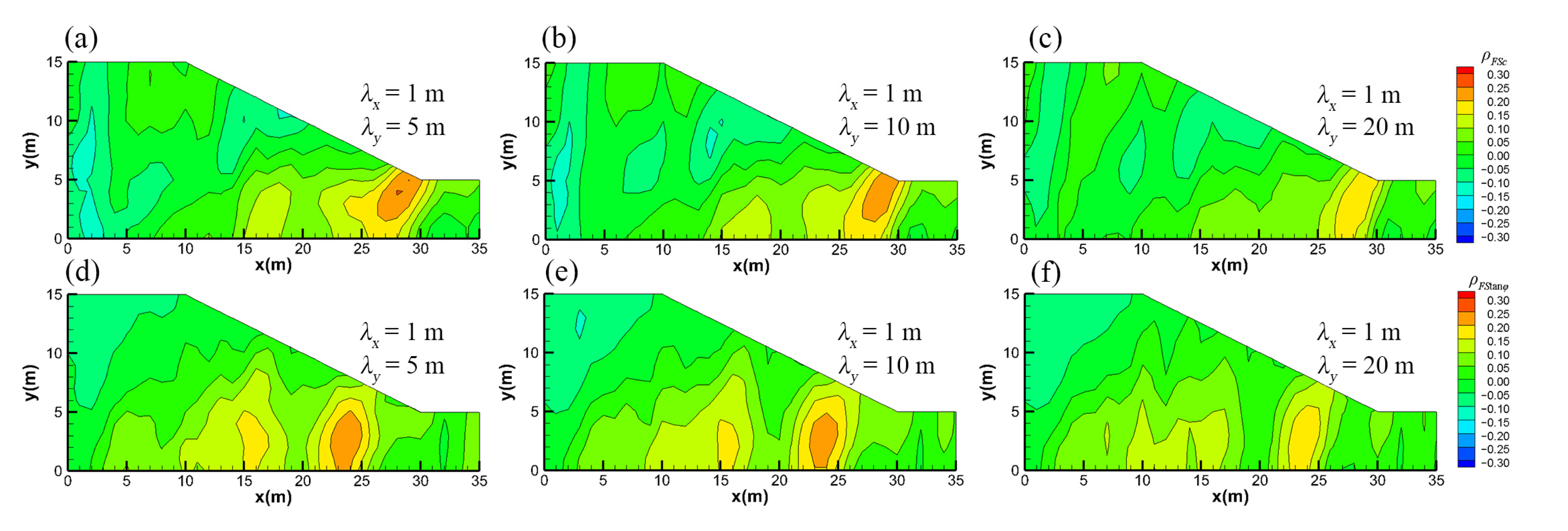
Figure 7 shows the cross-correlation map between FS and shear strength parameters (c and tanφ) with different λy values when the slope has vertically stratified formations. Figure 7a–c illustrate the cross-correlation maps between FS and c, and λy of c with 5, 10, and 20 m, respectively, while their horizontal correlation scales are 1 m. These figures indicate a distinctly positive correlation between FS and c at the toe of the slope. Furthermore, as λy increases, the high correlation area becomes more concentrated and vertical, and the cross-correlation value weakens slightly.
Figure 7d–f demonstrate the cross-correlation maps between FS and tanφ, and λy of tanφ equal to 5, 10, and 20 m, respectively. We observe that FS and tanφ are positively correlated at the area x = 20 to 25 m and y = 0 to 5 m, and the cross-correlation decreases slightly as λy increases.
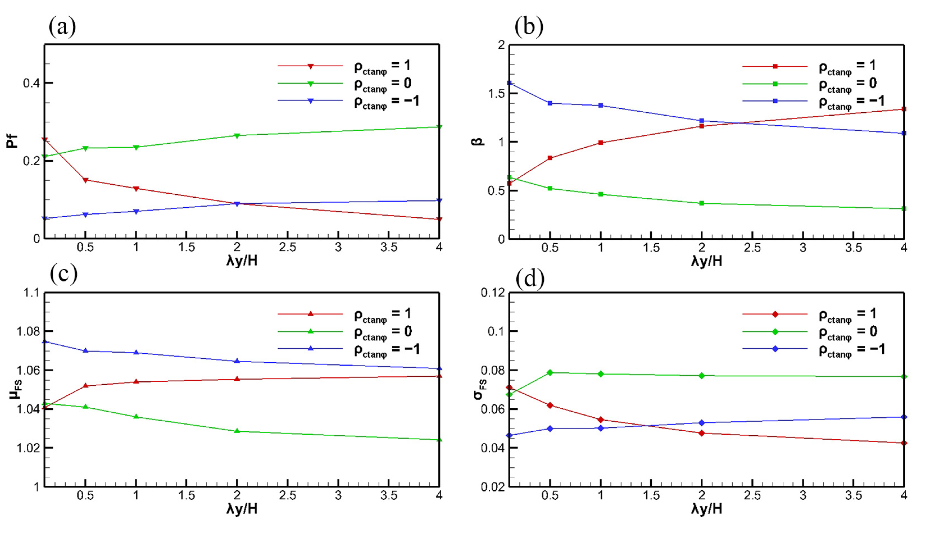
The behaviors of pf, β, μFS, and σFS in the slopes with longer vertical correlation scales than the horizontal one as a function of λy/H (the vertical correlation scale normalized by the height of the slope, H) are displayed in Figure 8a–c, and d, respectively. First, we notice that the value of probability failure (pf) in this case is much less than that in the horizontal layering slope (i.e., Figure 8a vs. Figure 6a), regardless of the effects of various factors as in Figure 6. In other words, vertical stratification (the orientation of the large-scale structures) plays a more dominant role than the others do in slope stability.
Nevertheless, Figure 8 shows that when ρctanφ is 1 (the red line), with the increase in λy, pf and σFS decrease, and μFS and β increase, indicative of the fact that as λy increases, the stability of the slope increases and the uncertainty of the evaluation decreases. This result stems from the fact that when a slope is vertically layered, the high-strength layer controls the stability, similar to anti-slip piles. The longer λy means that the layer with high strength is extensive, and when ρctanφ is 1, the c is large and so is φ large, and the anti-slip pile can be effective, leading to high slope stability.
When ρctanφ is 0 or −1 (the green and blue line in Figure 8), the increase in λy leads to increases in pf and σFS, and it decreases μFS and β values, suggesting that increasing λy worsens the stability of the slope and increases the uncertainty of the evaluation. These trends are the opposite of when ρctanφ is 1, likely because c and tanφ are uncorrelated or perfectly negatively correlated, and the effect of anti-slip piles weakens.

4.3. Effects of the Number of Realizations in MCS

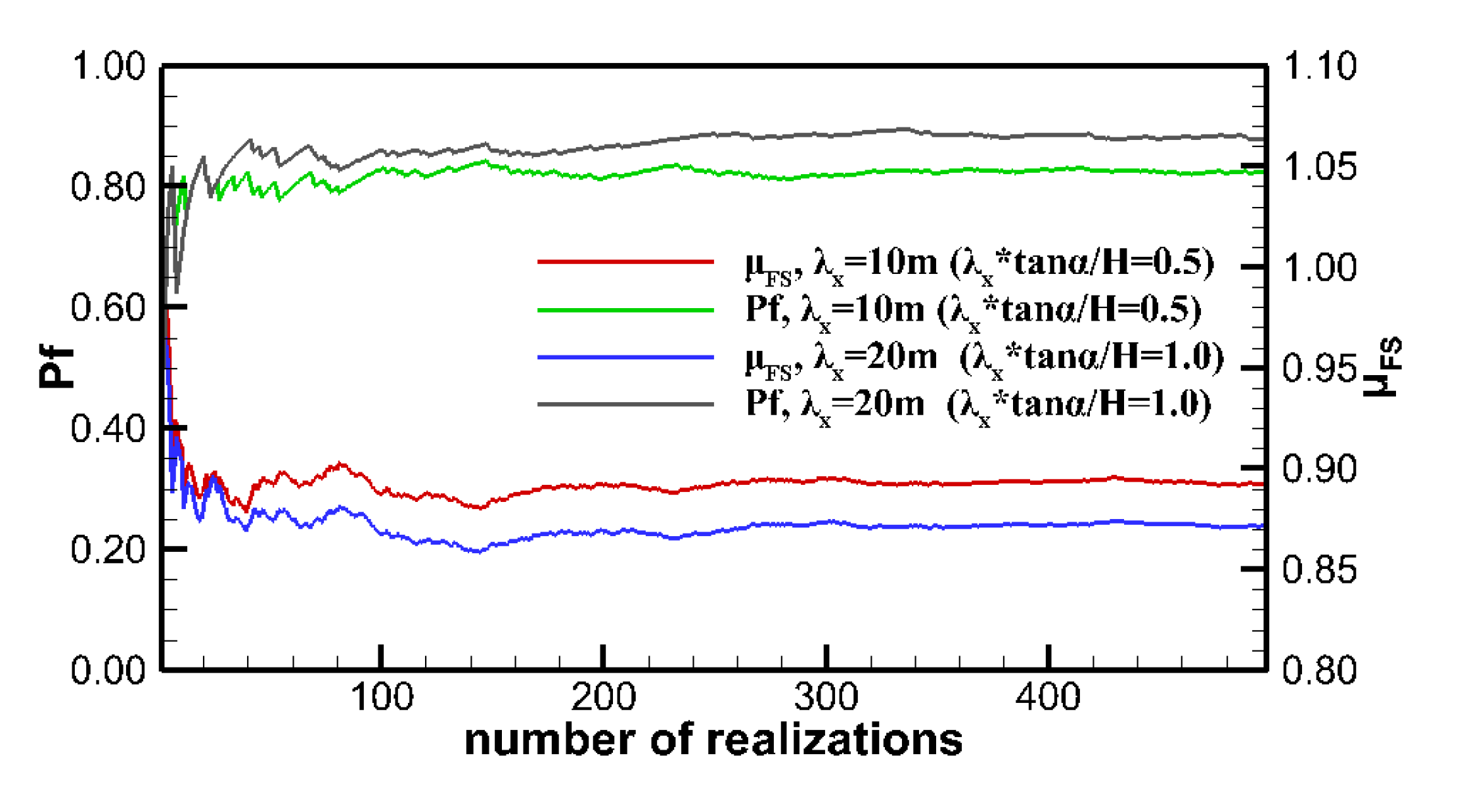
All the results above are from 500 MCS. To ensure that the number of simulations is sufficient to obtain representative results, we plot Figure 9 to show the effect of the number of realizations on pf and μFS at λx = 10 m and 20 m, respectively, and λy = 1 m, in these conditions, σFS are the maximums. As shown in the figure, the mean values of pf and μFS fluctuate widely within 150 realizations but stabilize after more than 300 realizations, certifying the adequacies of the number of realizations used in the MCS and the results’ representativeness.

5. Effects of Conditional Random Fields

To demonstrate that sampling in highly correlated zones (conditioning on the stochastic fields) reduces the uncertainty in the FS assessment, we conducted numerical experiments considering two cases where only the cohesion field is a stochastic process. Case 1 used the distribution of c in Figure 1a as the reference field, and Case 2 used the c distribution in Figure 1c. The mean, variance, and λy of the random fields in the two cases were identical, except that λx was different.
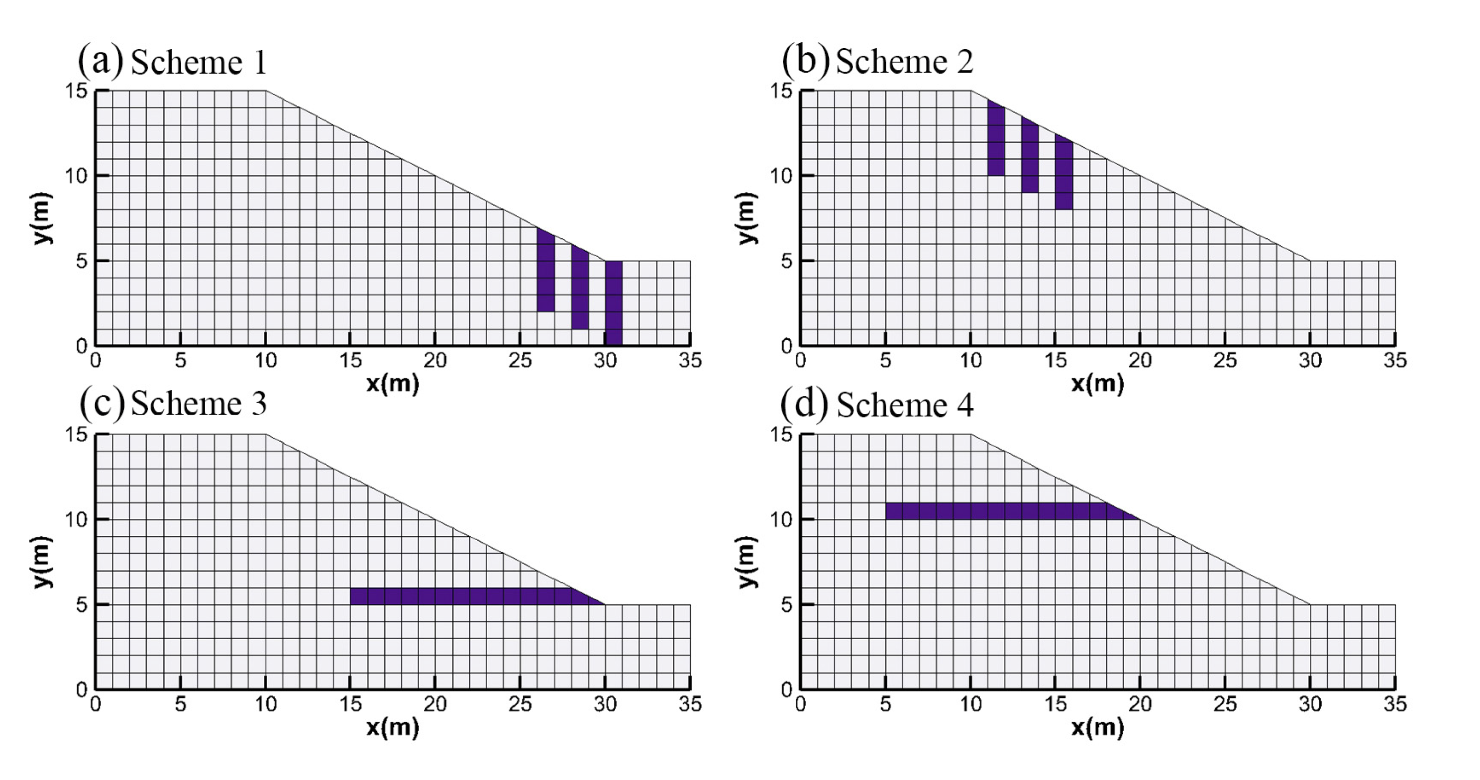
We considered four sampling schemes (Figure 10). In Scheme 1, samples were taken at the toe of the slope at three 5 m deep vertical boreholes (Figure 10a). In Scheme 2, the three boreholes were near the slope top (Figure 10b). Scheme 3 took samples over a 15 m borehole horizontally into the slope at the corner of the slope (Figure 10c). The fourth scheme sampled a 15 m borehole horizontally near the top of the slope (Figure 10d). These four schemes took a soil sample every meter to obtain 15 samples. As such, we could evaluate the effects of the same number of parameter values in different correlation areas for conditioning on the estimates of FS of the slope.
With the sampled data, 500 realizations of the conditional random field corresponding to each sampling scheme were generated using the Kriging Superposition Approach (KSA) [43,44]. The resulting conditional realizations honored the sampled values at the sampled locations and retained the specified spatial statistics of the random fields. Afterward, we used them to conduct MCS as the previous unconditional MCS, and the results are summarized in Table 2.
The reference FS of Case 1 is 1.031. The μFS of sampling Scheme 3 is the closest to the FS of the reference since the sampling area is primarily in the high correlation region. Sampling Scheme 1, which samples a smaller portion of the highly correlated region, yields μFS value that is the second closest to the reference value. Since sampling Schemes 2 and 4 cover the minimal correlation between the parameters and FS, they yield a μFS that differs significantly from the reference value and is close to the μFS of the unconditional random simulation, indicative of their ineffectiveness for defining the actual factor of safety.
For Case 2, the reference FS is 0.922. The results of the conditional MCS are similar to Case 1, and the mean and standard deviation of FS are the best for sampling Scheme 3. Moreover, due to the apparent layered structure of Case 2 (λx = 5 m), Scheme 3 with horizontal borehole sampling yields significantly better results than the other three schemes. As expected, the uncertainty in the FS evaluated for sampling Scheme 3, which samples the most highly correlated areas, is the smallest in both Case 1 and Case 2. That is, sampling the high correlation areas’ parameters is critical for evaluating slope stability because it reduces uncertainty significantly more than sampling in other regions. As demonstrated in this example, cross-correlation analysis guides optimal borehole placement locations. Furthermore, we could suggest that focusing on the high correlation areas for slope reinforcement measures is essential since the same reinforcement measures will be more effective in the high correlation areas than in the low correlation areas.

6. Conclusions

Cross-correlation analysis of the shear strength parameters and FS of statistically anisotropic heterogeneous slopes shows that the large-scale heterogeneity structures dominate the stability of a slope. Specifically, with the given mean and variance of the shear strength parameters, the probability of failure of slopes with a long vertical correlation scale (vertical structure) is much smaller than that with a long horizontal correlation scale (horizontal structure).
In statistically isotropic parameter fields, the distributions of the high correlation areas of ρFSc and ρFStanφ are different: the former distributes at the toe and top of the slope, and the latter in the interior of the slope.
For the slope with the long horizontal correlation scale, the high correlation area of shear strength parameters with FS is located at the toe of the slope and distributed horizontally. The larger λx is, the longer the extension of the area in the horizontal direction is. In addition, when c and tanφ are positively correlated or uncorrelated, the larger λx is, and the less stable the slope is. When c and tanφ are perfectly negatively correlated, the effect of λx on the stability of the slope decreases.
In the slope with a long vertical correlation scale, the high correlation area of the shear strength parameter with FS is located at the toe of the slope and distributed vertically. With the increase in λy, the correlation in the high correlation region slightly decreases, and the region’s distribution becomes more vertical than others. Moreover, when c and tanφ are positively correlated, the larger λy is, and the more stable the slope is. When c and tanφ are negatively correlated or uncorrelated, the larger λy is, and the less stable the slope is.
This study further demonstrates that sampling in high cross-correlation regions can reduce the uncertainty in slope stability analysis. In addition, when the slope has an apparent layered structure (statistical anisotropy), the sampling direction consistent with its structure is recommended.
In summary, to evaluate the stability of a slope, first, one must detect the orientation of the large-scale structures (i.e., long correlation scales). The knowledge of the correlation between c and tanφ becomes essential, which dictates the probability of slope failure in the slopes with horizontal layering. The cross-correlation analysis presented in this study yields the location of the critical areas where shear strength parameters affect slope stability. Furthermore, these high cross-correlation regions guide the optimal borehole placement locations to reduce uncertainty in slope stability analysis and even for the selection of slope stability reinforcement locations.

Author Contributions

Conceptualization, Y.L. and T.-C.J.Y.; methodology, T.-C.J.Y. and Y.L.; software, Y.L. and T.-C.J.Y.; validation, F.Z. and M.D.; data curation, X.H.; writing—original draft preparation, Y.L.; writing—review and editing, T.-C.J.Y. and X.H. All authors have read and agreed to the published version of the manuscript.

Funding

This study was financially supported by the Fundamental Research Funds for the Central Universities (Grant No. 2019B60414). The corresponding author acknowledges the support of the U.S. National Science Foundation (Grant EAR1931756).

Data Availability Statement

The data that support the findings of this study are available from the corresponding author upon request.

Conflicts of Interest

The authors declare no conflict of interest.

References

  1. Rackwitz, R. Reviewing probabilistic soils modelling. Comput. Geotech. 2000, 26, 199–223. [Google Scholar] [CrossRef]
  2. Nielsen, D.R.; Biggar, J.W.; Erh, K.T. Spatial Variability of Field-measured Soil-water Characteristics. Hilgardia 1985, 42, 215–260. [Google Scholar] [CrossRef] [Green Version]
  3. Phoon, K.K.; Kulhawy, F.H. Characterization of geotechnical variability. Can. Geotech. J. 1999, 36, 612–624. [Google Scholar] [CrossRef]
  4. Xiao, T.; Li, D.Q.; Cao, Z.J.; Au, S.K.; Phoon, K.K. Three-dimensional slope reliability and risk assessment using auxiliary random finite element method. Comput. Geotech. 2016, 79, 146–158. [Google Scholar] [CrossRef] [Green Version]
  5. Jiang, S.H.; Huang, J.; Griffiths, D.V.; Deng, Z.P. Advances in reliability and risk analyses of slopes in spatially variable soils: A state-of-the-art review. Comput. Geotech. 2022, 141, 104498. [Google Scholar] [CrossRef]
  6. Griffiths, D.V.; Fenton, G.A. Probabilistic Slope Stability Analysis by Finite Elements. J. Geotech. Geoenviron. Eng. 2004, 23, 1390–1392. [Google Scholar] [CrossRef] [Green Version]
  7. Qi, X.H.; Li, D.Q. Effect of spatial variability of shear strength parameters on critical slip surfaces of slopes. Eng. Geol. 2018, 239, 41–49. [Google Scholar] [CrossRef]
  8. Griffiths, D.V.; Huang, J.; Fenton, G.A. Influence of spatial variability on slope reliability using 2-D random fields. J. Geotech. Geoenviron. Eng. 2009, 135, 1367–1378. [Google Scholar] [CrossRef] [Green Version]
  9. Jiang, S.H.; Li, D.Q.; Zhang, L.M.; Zhou, C.B. Slope reliability analysis considering spatially variable shear strength parameters using a non-intrusive stochastic finite element method. Eng. Geol. 2014, 168, 120–128. [Google Scholar] [CrossRef]
  10. Cho, S.E. Effects of spatial variability of soil properties on slope stability. Eng. Geol. 2007, 92, 97–109. [Google Scholar] [CrossRef]
  11. Ciurleo, M.; Cascini, L.; Calvello, M. A Comparison of Statistical and Deterministic Methods for Shallow Landslide Susceptibility Zoning in Clayey Soils. Eng. Geol. 2017, 223, 71–81. [Google Scholar] [CrossRef]
  12. Tropeano, G.; Silvestri, F.; Ausilio, E. An Uncoupled Procedure for Performance Assessment of Slopes in Seismic Conditions. Bull. Earthq. Eng. 2017, 15, 3611–3637. [Google Scholar] [CrossRef] [Green Version]
  13. Miao, F.; Wu, Y.; Xie, Y.; Li, Y. Prediction of Landslide Displacement with Step-like Behavior Based on Multialgorithm Optimization and a Support Vector Regression Model. Landslides 2018, 15, 475–488. [Google Scholar] [CrossRef]
  14. Miao, F.; Zhao, F.; Wu, Y.; Li, L.; Török, Á. Landslide Susceptibility Mapping in Three Gorges Reservoir Area Based on GIS and Boosting Decision Tree Model. Stoch. Environ. Res. Risk Assess. 2023, 4, 1–21. [Google Scholar] [CrossRef]
  15. Yeh, T.C.J.; Ye, M.; Khaleel, R. Estimation of effective unsaturated hydraulic conductivity tensor using spatial moments of observed moisture plume. Water Resour. Res. 2005, 41, 1–12. [Google Scholar] [CrossRef]
  16. Cai, J.S.; Yeh, T.C.J.; Yan, E.C.; Tang, R.X.; Hao, Y.H. Design of borehole deployments for slope stability analysis based on a probabilistic approach. Comput. Geotech. 2021, 133, 103909. [Google Scholar] [CrossRef]
  17. Gao, X.; Yan, E.C.; Yeh, T.C.J.; Wang, Y.L.; Cai, J.S.; Hao, Y.H. Sequential back analysis of spatial distribution of geomechanical properties around an unlined rock cavern. Comput. Geotech. 2018, 99, 177–190. [Google Scholar] [CrossRef]
  18. Mao, D.; Yeh, T.C.J.; Wan, L.; Lee, C.H.; Hsu, K.C.; Wen, J.C.; Lu, W. Cross-correlation analysis and information content of observed heads during pumping in unconfined aquifers. Water Resour. Res. 2013, 49, 713–731. [Google Scholar] [CrossRef]
  19. Sun, R.; Yeh, T.C.J.; Mao, D.; Jin, M.; Lu, W.; Hao, Y. A temporal sampling strategy for hydraulic tomography analysis. Water Resour. Res. 2013, 49, 3881–3896. [Google Scholar] [CrossRef]
  20. Zhao, C.; Gong, W.; Li, T.; Juang, C.H.; Tang, H.; Wang, H. Probabilistic characterization of subsurface stratigraphic configuration with modified random field approach. Eng. Geol. 2021, 288, 106138. [Google Scholar] [CrossRef]
  21. Wang, M.; Tang, X.; Li, D.; Qi, X. Subset simulation for efficient slope reliability analysis involving copula- based cross-correlated random fields. Comput. Geotech. 2020, 118, 103326. [Google Scholar] [CrossRef]
  22. Gong, W.; Zhao, C.; Juang, C.H.; Zhang, Y.; Tang, H.; Lu, Y. Coupled characterization of stratigraphic and geo-properties uncertainties—A conditional random field approach. Eng. Geol. 2021, 294, 106348. [Google Scholar] [CrossRef]
  23. Ye, M.; Khaleel, R.; Yeh, T.C.J. Stochastic analysis of moisture plume dynamics of a field injection experiment. Water Resour. Res. 2005, 41, 1–13. [Google Scholar] [CrossRef] [Green Version]
  24. Cruden, D.M.; Varnes, D.J. Landslide Types and Processes. In Landslides: Investigation and Mitigation; National Academy Press: Washington, WA, USA, 1996; Volume 247, pp. 36–75. [Google Scholar]
  25. Terzaghi, K. Mechanism of Landslides. In Application of Geology to Engineering Practice; Geological Society of America: New York, NY, USA, 1950; pp. 83–123. [Google Scholar]
  26. Leroueil, S. Natural Slopes and Cuts: Movement and Failure Mechanisms. Géotechnique 2001, 51, 197–243. [Google Scholar] [CrossRef]
  27. Cai, J.S.; Yan, E.C.; Yeh, T.C.J.; Zha, Y.Y.; Liang, Y.; Huang, S.Y.; Wang, W.K.; Wen, J.C. Effect of spatial variability of shear strength on reliability of infinite slopes using analytical approach. Comput. Geotech. 2017, 81, 77–86. [Google Scholar] [CrossRef] [Green Version]
  28. Johari, A.; Fooladi, H. Simulation of the conditional models of borehole’s characteristics for slope reliability assessment. Transp. Geotech. 2022, 35, 100778. [Google Scholar] [CrossRef]
  29. Liu, L.L.; Cheng, Y.M.; Zhang, S.H. Conditional random field reliability analysis of a cohesion-frictional slope. Comput. Geotech. 2017, 82, 173–186. [Google Scholar] [CrossRef]
  30. Yang, R.; Huang, J.; Griffiths, D.V.; Sheng, D. Probabilistic Stability Analysis of Slopes by Conditional Random Fields. In Proceedings of the Geo-Risk, Denver, CO, USA, 4–7 June 2017; American Society of Civil Engineers: Reston, VA, USA, 2017; pp. 450–459. [Google Scholar] [CrossRef]
  31. Johari, A.; Fooladi, H. Comparative study of stochastic slope stability analysis based on conditional and unconditional random field. Comput. Geotech. 2020, 125, 103707. [Google Scholar] [CrossRef]
  32. Yeh, T.C.J.; Khaleel, R.; Carroll, K.C. Flow through Heterogeneous Geologic Media; Cambridge University Press: New York, NY, USA, 2015; ISBN 9781139879323. [Google Scholar]
  33. Gutjahr, A.L. Fast fourier transforms for random field generation. In New Mexico Tech Project Report 4-R58-2690R; New Mexico Institute of Mining and Technology: Socorro, NM, USA, 1989; Volume 29, pp. 2385–2397. [Google Scholar]
  34. Robin, M.J.L.; Gutjahr, A.L.; Sudicky, E.A.; Wilson, J.L. Cross-correlated random field generation with the direct Fourier Transform Method. Water Resour. Res. 1993, 29, 2385–2397. [Google Scholar] [CrossRef]
  35. Elia, G.; Falcone, G.; Cotecchia, F.; Rouainia, M. Analysis of the Effects of Seasonal Pore Pressure Variations on the Slope Stability Through Advanced Numerical Modelling. In Lecture Notes in Civil Engineering; Springer International Publishing: Berlin/Heidelberg, Germany, 2020; Volume 40, pp. 184–194. ISBN 9783030213596. [Google Scholar]
  36. Pedone, G.; Tsiampousi, A.; Cotecchia, F.; Zdravkovic, L. Coupled Hydro-Mechanical Modelling of Soil–Vegetation–Atmosphere Interaction in Natural Clay Slopes. Can. Geotech. J. 2022, 59, 272–290. [Google Scholar] [CrossRef]
  37. Gao, X.; Yan, E.-C.; Yeh, T.-C.J.; Wang, Y.; Liang, Y.; Hao, Y. Reliability Analysis of Hydrologic Containment of Underground Storage of Liquefied Petroleum Gas. Tunn. Undergr. Sp. Technol. 2018, 79, 12–26. [Google Scholar] [CrossRef]
  38. Zhang, X.; Bi, J.; Guo, D.; Li, Z. Numerical Simulation of Stability Analysis of Soil Slope Using General Particle Dynamics with Elastic-plastic Constitutive Model. Mater. Des. Process. Commun. 2019, 1, e51. [Google Scholar] [CrossRef] [Green Version]
  39. Griffiths, D.V.; Lane, P.A. Slope stability analysis by finite elements. Geotechnique 1999, 49, 387–403. [Google Scholar] [CrossRef]
  40. Smith, I.M.; Griffiths, D.V.; Margetts, L. Programming the Finite Element Method; John Wiley & Sons: Chichester, UK, 2014; ISBN 9781119973348. [Google Scholar]
  41. Morgenstern, N.R.; Price, V.E. The analysis of the stability of general slip surfaces. Geotechnique 1965, 15, 79–93. [Google Scholar] [CrossRef]
  42. Gao, X.; Chuan Yan, E.; Yeh, T.C.J.; Cai, J.S.; Liang, Y.; Wang, M. A geostatistical inverse approach to characterize the spatial distribution of deformability and shear strength of rock mass around an unlined rock cavern. Eng. Geol. 2018, 245, 106–119. [Google Scholar] [CrossRef]
  43. Gao, X.; Yeh, T.C.J.; Yan, E.C.; Wang, Y.L.; Hao, Y. Conditional mean, effective, and realizations of hydraulic conductivity fields. J. Hydrol. 2021, 592, 125606. [Google Scholar] [CrossRef]
  44. Yeh, T.C.J. Stochastic modelling of groundwater flow and solute transport in aquifers. Hydrol. Process. 1992, 6, 369–395. [Google Scholar] [CrossRef] [Green Version]
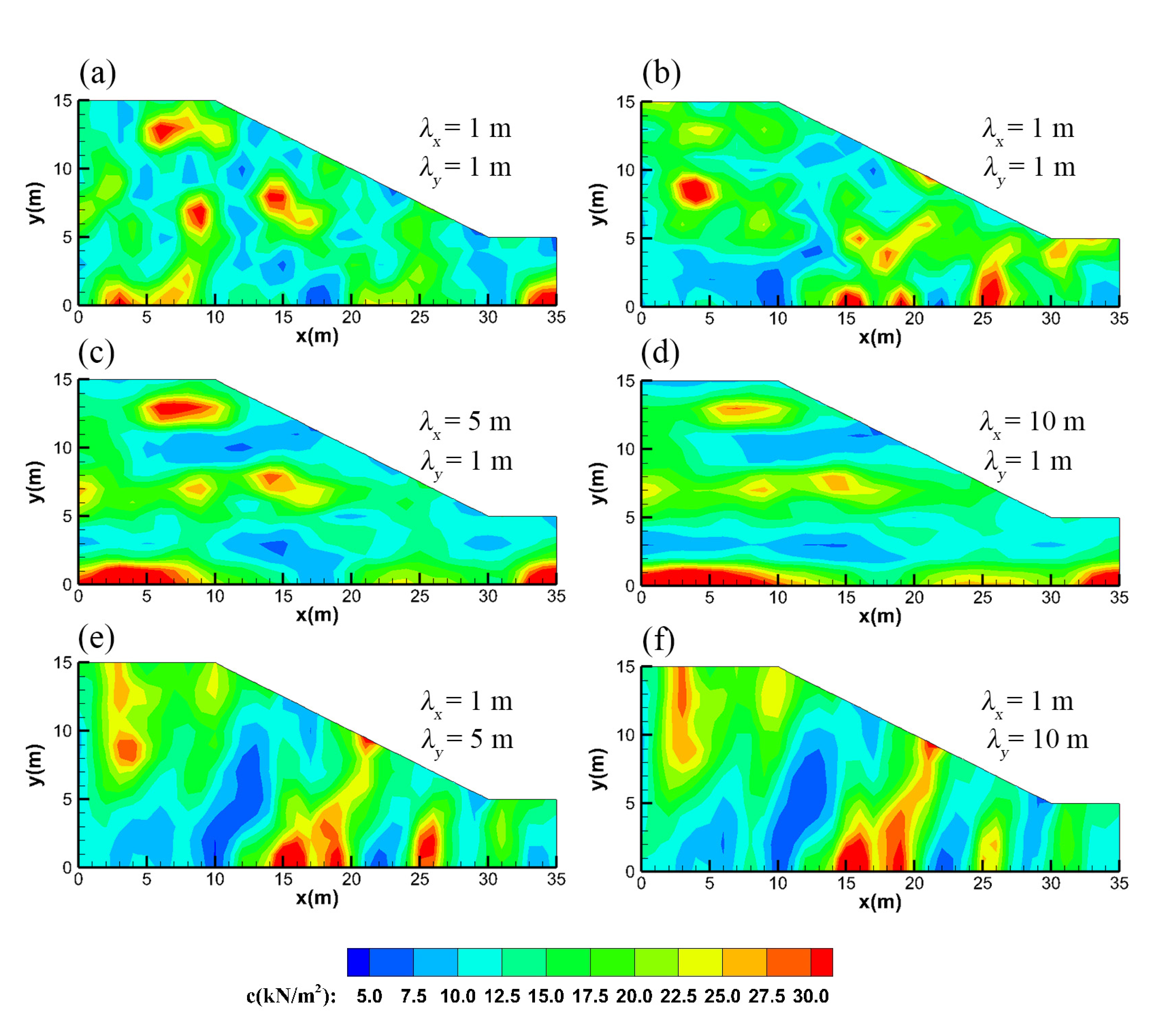
Figure 1. Numerically generated realizations of c in different correlation scales: (a,b) λx = λy = 1 m, with different random seed, (c) λx = 5 m, λy = 1 m, (d) λx = 10 m, λy = 1 m, (e) λx = 1 m, λy = 5 m, and (f) λx = 1 m, λy = 10 m.
Water 15 01050 g001
Figure 2. The synthetic slope model.
Water 15 01050 g002
Figure 3. (a) Cross-correlation map of FS and c, (b) Cross-correlation map of FS and tanφ for statistical isotropy.
Water 15 01050 g003
Figure 4. (a) Sensitivity map of FS to c, (b) sensitivity map of FS to tanφ.
Water 15 01050 g004
Figure 5. Cross-correlation maps of FS and c (ac) and tanφ (df) under three different horizontal statistical anisotropic correlation scales.
Water 15 01050 g005
Figure 6. (ad) are pf, β, μFS and σFS of FS obtained by MCS for different λx and ρctanφ values.
Water 15 01050 g006
Figure 7. Cross-correlation maps of FS and c (ac) and tanφ (df) under three different vertical statistical anisotropic correlation scales.
Water 15 01050 g007
Figure 8. (ad) are pf, β, μFS, and σFS of FS obtained by MCS for different λy and ρctanφ values.
Water 15 01050 g008
Figure 9. Pf and μFS, when λy = 1 m and λx = 10 m and 20 m, respectively, as functions of the number of realizations.
Water 15 01050 g009
Figure 10. Borehole locations of four sampling schemes.
Water 15 01050 g010
Table 1. Prior statistics of shear strength and other parameters for the numerical model.
ParametersValues
Mean of cohesion, μc15 kN/m2
Coefficient of variation of cohesion, COVc0.5
Mean of friction angle, μφ10°
Coefficient of variation of friction angle, COVφ0.5
Dilation angle, ψ
Young’s modulus, E1 × 105 kPa
Poisson’s ratio, υ0.3
Unit weight, γ20 kN/m3
Table 2. The results of conditional MCS.
Scheme 1Scheme 2Scheme 3Scheme 4
μFS of Case 11.0331.0411.0311.040
σFS of Case 10.0660.0720.0580.072
μFS of Case 20.9350.9390.9240.935
σFS of Case 20.0940.1050.0820.112
Disclaimer/Publisher’s Note: The statements, opinions and data contained in all publications are solely those of the individual author(s) and contributor(s) and not of MDPI and/or the editor(s). MDPI and/or the editor(s) disclaim responsibility for any injury to people or property resulting from any ideas, methods, instructions or products referred to in the content.