Effects of Wave Height, Period and Sea Level on Barred Beach Profile Evolution: Revisiting the Roller Slope in a Beach Morphodynamic Model

Abstract

Sandbars are commonly observed on sandy coasts, and they can prevent erosion on the beach face. Better prediction of sandbar evolution is necessary for coastal management and beach nourishment. In this study, a process-based morphodynamic model is used to reproduce the barred beach profile evolution in the Duck94 field experiments. The importance of the wave roller slope parameter in the model is revisited. Six idealized numerical experiments are set to investigate the effect of wave heights, wave periods and sea levels on sandbar migrations. By implementing two recent cross-shore varying roller slope formulas, the models achieved fair-to-good performances. It was found that the variations of sandbar morphological evolution are mainly controlled by the cross-shore varying roller slope. An increase in the wave height or a decrease in the wave period would lead to a more rapid and further-offshore migration of the sandbar. When the sea level variations are much smaller than the water depth over the sandbar, the effect of sea level changes on the sandbar migration is negligible, though a lower sea level would cause more erosion on the beach face.

1. Introduction

The sandy coast is the interface between land and sea, having rich sediment resources, fisheries and tourism resources, and a relatively developed economy. Two-thirds of the world’s population is concentrated within 100 km of the coast [1]. The sandbar is a typical geomorphic element on sandy coasts and can protect the beach face by triggering wave breaking and energy dissipation. It usually forms under large wave conditions in winter and disappears in summer, often known as the winter profile and summer profile [2]. The migration and morphological evolution of the sandbar are driven by the incoming waves, and it tends to be in equilibrium when the incoming waves are stable [3]. A better understanding and better prediction of barred beach profile evolution are necessary for sandy beach management and restoration.

Empirical models can directly reproduce the equilibrium barred beach profile, but, thus far, these models do not include morphological evolution processes and their physical consequences [4]. Phase-resolving models simulate hydrodynamics and sediment transport patterns at intra-wave scales to provide very detailed and precise predictions of hydrodynamics [5]. However, these models are always computationally expensive for simulating the beach profile evolution at prototype scale. In contrast, phase-averaged models can reproduce beach morphodynamics at time scales from weeks to months [6,7,8,9,10,11]. These models are usually suitable for engineering practices due to their high computational accuracy and efficiency. Phase-averaged models often use parameterizations to quantify some key physical processes such as the energy dissipation due to wave breaking, surface roller evolution and bedload sediment transport [7].

The slope of the wave surface roller is a key parameter in the beach morphodynamic model. It represents the energy dissipation during roller evolution and thus controls the intensity of the undertow. In most previous models, the roller slope was recognized as a tunable parameter and set as a constant over the calculation domain. For example, the roller slope was set as 0.1 for the original version of the XBeach [7]. Reniers et al. [12] used 0.05 in their RR94 model to model the vertical flow structure during a Sandy Duck field experiment. Recently, Rafati et al. [13] modified the empirical formula of the roller slope from Walstra et al. [14] and implemented it in the XBeach model. They found that using a cross-shore varying roller slope can improve undertow prediction in the sandbar region.

The morphological evolution of the sandbar is sensitive to wave height, wave period and sea level. Wave height and period are representations of wave power. Wave period can affect the beach response to incoming waves. For example, wave period is an important factor in the contribution of waves to sediment resuspension [15], and it also can affect the formation of rip currents at macrotidal pocket beaches [16]. The sea level plays an important role in barred beach profile evolution since it affects the upper limit of wave runup as well as the wave breaking intensity [17,18]. Therefore, the objective of this study is to revisit the roller slope in the beach morphodynamic model and to analyze the effect of wave height, period and sea level on sandbar morphological evolution. The paper is organized as follows. Section 2 provides a brief description of field datasets and model description. Results of the model vs. data comparison and the effect of wave height, period and sea level on barred beach profile evolution are provided in Section 3. Finally, conclusions are drawn in Section 4.

2. Methodology

2.1. Process-Based Numerical Model

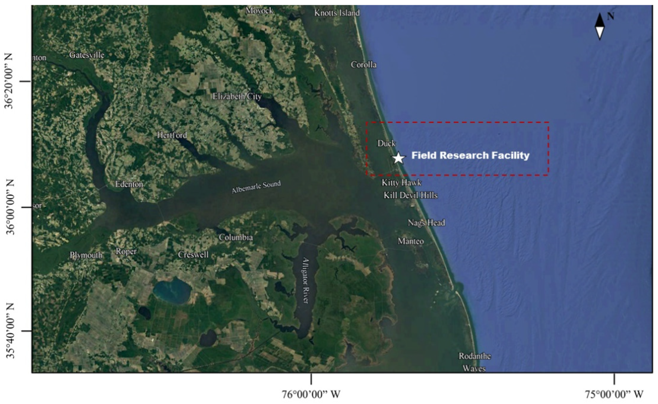
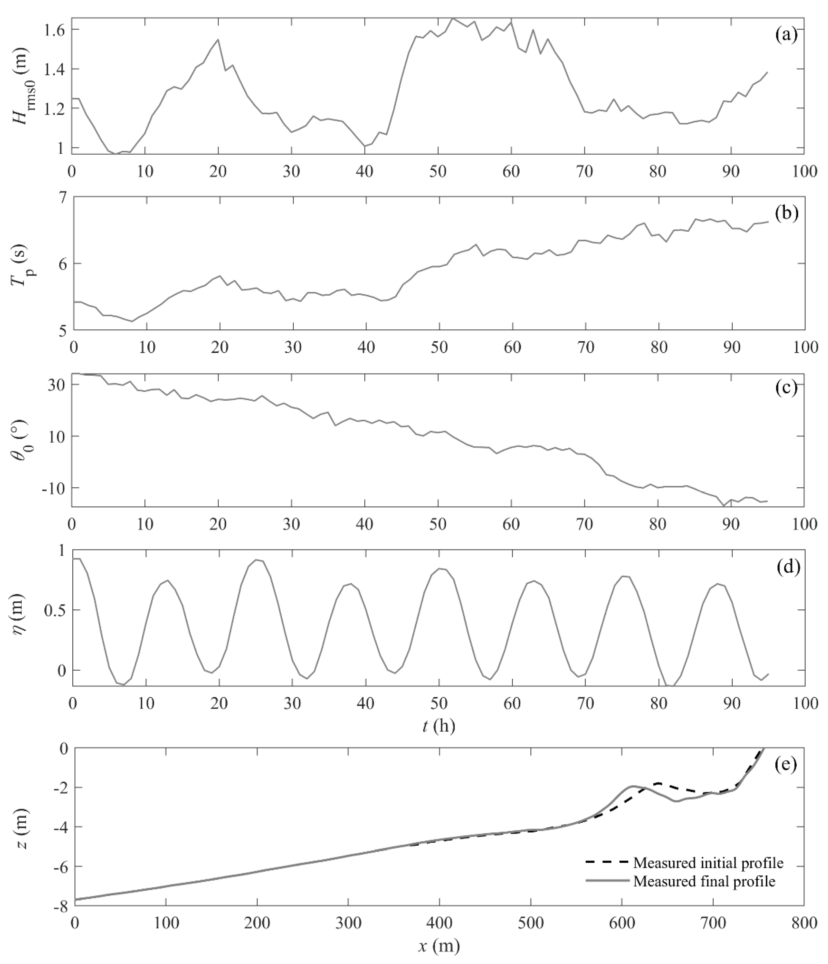
The process-based numerical model used in this study, CROSPE, was first developed by Zheng et al. [11] to account for coastal sandbar migration caused by discrepancies in sediment transport rates in the cross-shore direction. In the model, various driving forces at different time scales are involved, e.g., nonlinear waves, surface rollers, offshore compensating currents, gravity effect and bottom boundary layer streaming. In recent years, the performance of the model in predicting the formation of the equilibrium barred beach profile and the onshore migration of the shoreface nourishment has been proved [19,20,21].

The CROSPE model solves the wave energy conservation and roller energy conservation equation for the RMS wave height and roller energy, respectively. The time-averaged wave setup is calculated using a depth-integrated momentum equation considering the contribution of the excess wave roller energy. The instantaneous flow velocity is solved by a first-order wave–current momentum equation. The sediment transport module solves an advection–diffusion equation for the sediment concentration and employs a Meyer-Peter–Muller type formula to estimate the instantaneous bedload transport rate. Finally, the bottom profile evolution is estimated with the Exner equation.

The wave roller slope, defined as the mean slope angle from the still water level to the wave (roller) crest, is a key parameter in coastal morphodynamic models [11,13,22,23]. Details of wave and roller modules are provided below, and more information about the CROSPE model can be found in Zheng et al. and Li et al. [3,11].

The wave energy conservation equation considering the loss of wave energy induced by wave breaking and bottom friction is written as follows:

$$\frac{\partial \left(E_w{c}_g\right)}{\partial x}=-D_b-D_f$$

(1)

where E_w means the wave energy density, c_g is the wave group velocity, D_b is the wave breaking energy dissipation, D_f is the energy dissipation due to bottom friction. The wave breaking energy dissipation D_b was estimated by using the model of Baldock et al. [24] in this study, though other parametric wave breaking models can be used as alternatives [25,26]. Compared with the original version, the present model updates the representation of the breaker index in the parametric wave breaking dissipation module [27]. The updated breaker index formula exhibits composite dependence on both offshore wave steepness and local normalized water depth; it reads as follows:

$$\gamma =(237s_0^2-34.81s_0+1.46)\exp [1.96\ln (38.64s_0)\times kh]$$

(2)

where γ is the breaker index, s₀ represents the offshore wave steepness, k is the wave number, h means the local water depth. The new breaker index formula was chosen because it considers both the breaking intensification mechanism and the breaking resistance mechanism. Zhang et al. [27] found that implementation of this new γ formula in the parametric wave model of Baldock et al. [24] can systematically reduce the median percentage error of wave height prediction by 10–24%.

The roller energy conservation equation taking the input energy from wave breaking and the energy dissipation with the wave roller evolution into account is written as follows:

$$\frac{\partial \left(2E_r{c}_p\right)}{\partial x}=D_b-D_r$$

(3)

where E_r means the roller energy density, c_p means the wave celerity, D_r is the roller energy dissipation. The roller energy dissipation D_r is estimated as

$$D_r=\frac{2g{E}_r\sin \beta }{c_p}$$

(4)

where β is the roller slope, g is the gravity acceleration. The roller slope is a key parameter that controls the amount of roller energy dissipation and thus affects the wave setup and undertow velocity. A constant value for β was commonly used in previous studies, e.g., 0.05 or 0.1 [12,28,29]. Recently, Zhang et al. [22] found that the roller slope increases as waves shoal and then decreases when waves break rather than being a constant value in the cross-shore direction. Then, a spatial-varying roller slope was proposed as follows:

$$\beta =\left\{\begin{array}{ll}\arctan (\frac{2H_{rms}}{L})& Ur\le 1\\ \arctan (2+0.6{(\log Ur)}^3\frac{H_{rms}}{L})& Ur>1\end{array}\right.$$

(5)

where Ur is the Ursell number, Ur = H_rmsL²/h³, L is wavelength calculated with the wave peak period. The Ursell number is an important indicator for the nonlinearity of surface gravity waves [30,31,32]. More recently, Rafati et al. [13] modified the formula for roller slope on the basis of Walstra et al. [14] and found that the modified, cross-shore varying roller slope formula is more precise in predicting undertow under energetic wave conditions than the constant one. The modified formula is written as follows:

$$\beta =\left\{\begin{array}{ll}0.03kh\frac{h-H_{rms}}{H_{rms}}<0.1& kh\ge 0.45\\ 0.1,& kh<0.45\end{array}\right.$$

(6)

where k is the wave number calculated by the iterative solution of the dispersion relation for linear waves. It can be found that the roller slope generally decreases with water depth in Equation (6), unlike in Equation (5) where there is no significant relationship between the roller slope and the water depth.

In the following section, the performances of cross-shore varying roller slope and constant roller slope in predicting barred beach profile evolution will be evaluated. In addition to the wave roller slope, the CROSPE model also contains three other calibrating parameters, i.e., the turbulence coefficient f_v, phase-shift angle φ and the Prandtl/Schmidt number σ_p. Details of the numerical schemes and iterative algorithms can be found in Zheng et al. [11].

2.2. Field Data

The data used in this study were collected during the Duck94 field experiment from September to October of 1994 near Duck, North Carolina, on a barrier island exposed to the Atlantic Ocean [33,34], as can be seen in Figure 1. Incident waves were measured from a 2D array of 15 bottom-mounted pressure sensors in 8 m water depth, carried out by the U.S. Army Corps of Engineers—Field Research Facility (FRF) [35,36].

As can be seen in Figure 2, 96 h measured data were used in this study, with t = 0 h (corresponding to 10 October 1994, 12:00 EST). The main reason for selecting this period for the modeling was that two energetic events were recorded (i.e., at t = 20 h and t = 50–65 h), which can drive obvious morphological changes. This period was also used in Li et al. [37]. The sediments on the beach were fine-to-medium, with grain size ranging from 0.15 mm to 0.29 mm. Unlike the sand–mud transitional beaches on South China coasts with a clear sand–mud transition line, the medium grain size of sands became a constant 0.2 mm when the beach level was lower than −1.5 m [8,38,39]. Two peaks occur in the time series of RMS wave height. The wave peak period and wave angle exhibited monotonic variations over the study period. The beach shape was single barred, with the primary sandbar located at x = 640 m and migrating offshore toward 600 m.

3. Results and Discussion

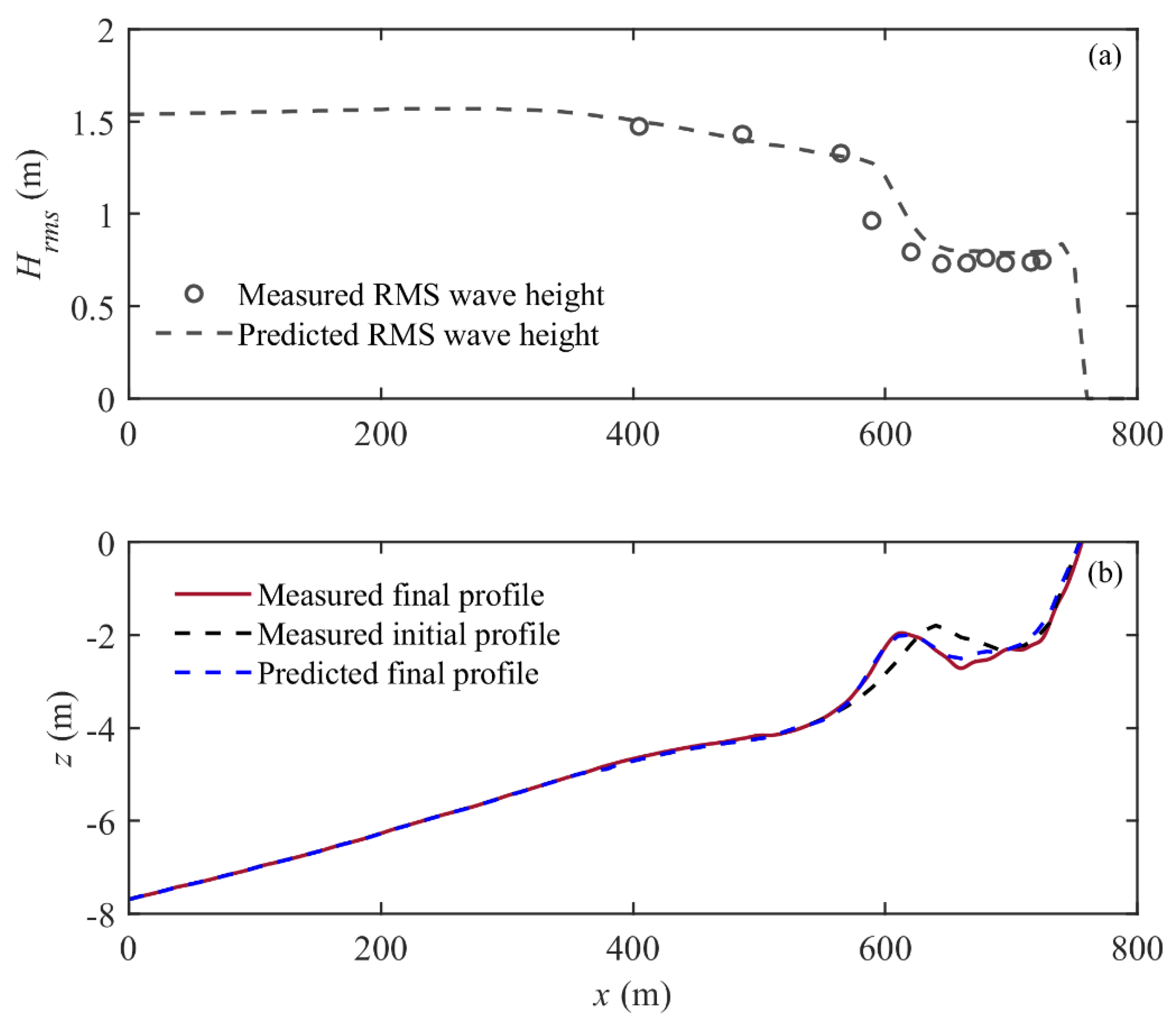
3.1. Model Calibration with Constant Roller Slope

Before model calibration, two error indexes were employed to quantify the model performance, i.e., root-mean-square error (RMSE) and Brier skill score (BSS), which are defined as follows:

$$\mathrm{RMSE}=\sqrt{\overline{{\left(R_t-O_t\right)}^2}}$$

(7)

$$\mathrm{BSS}=1-\frac{\overline{{\left(R_t-O_t\right)}^2}}{\overline{{\left(O_t-O_0\right)}^2}}$$

(8)

where R_t is the predicted final beach profile (or RMS wave height), O_t is the observed final beach profile, O₀ is the initial beach profile. Following van Rijn et al. [40], BSS = 0.1–0.3 means a poor fit, BSS = 0.3–0.6 means a fair fit, BSS = 0.6–0.8 means a good fit and, finally, BSS = 0.8–1.0 equals an excellent fit.

Model calibration with a constant roller slope was conducted in Li et al. [37]. A brief description is provided here: The roller slope was set as 0.08, and the turbulent coefficient f_v, phase-shift angle φ and the Prandtl/Schmidt number σ_p were set as 0.025, 30° and 1, respectively. As can be seen in Figure 3, good agreement was found between predicted and observed RMS wave height and beach profile evolution. The RMSE for the comparison of the RMS wave height at the end of the model was 0.11 m. The BSS for the comparison of the beach profile evolution was 0.92, implying that the performance of the model was excellent [37].

Although the use of a constant roller slope exhibited an excellent model performance, the choice of 0.08 seems arbitrary. The setting of a constant roller slope in the model contradicts the recent finding that the roller slope is temporally and spatially varying [22]. Constant roller slopes can vary from coast to coast and even vary at different time periods on the same coast. For example, Ruessink et al. [8] found that, using the constant roller slope of 0.1, the model can well reproduce the sandbar migration at the single-barred beaches in Duck94 experiments as well as at Hasaki, Kashima Coast, Japan. Li et al. [3] showed that using a constant roller slope of 0.06 in the model can both well reproduce the Duck94 experiment from 14 October 1994 to 18 October 1994 and the laboratory experiments on sandbar formation carried out by Roelvink and Stive [41]. It should be admitted, however, that the physical meaning of the wave roller slope is weakened during the model calibration. In the next section, formulas of roller slope varying in the cross-shore direction, i.e., with physical meanings, are implemented in the CROSPE model to test their performances.

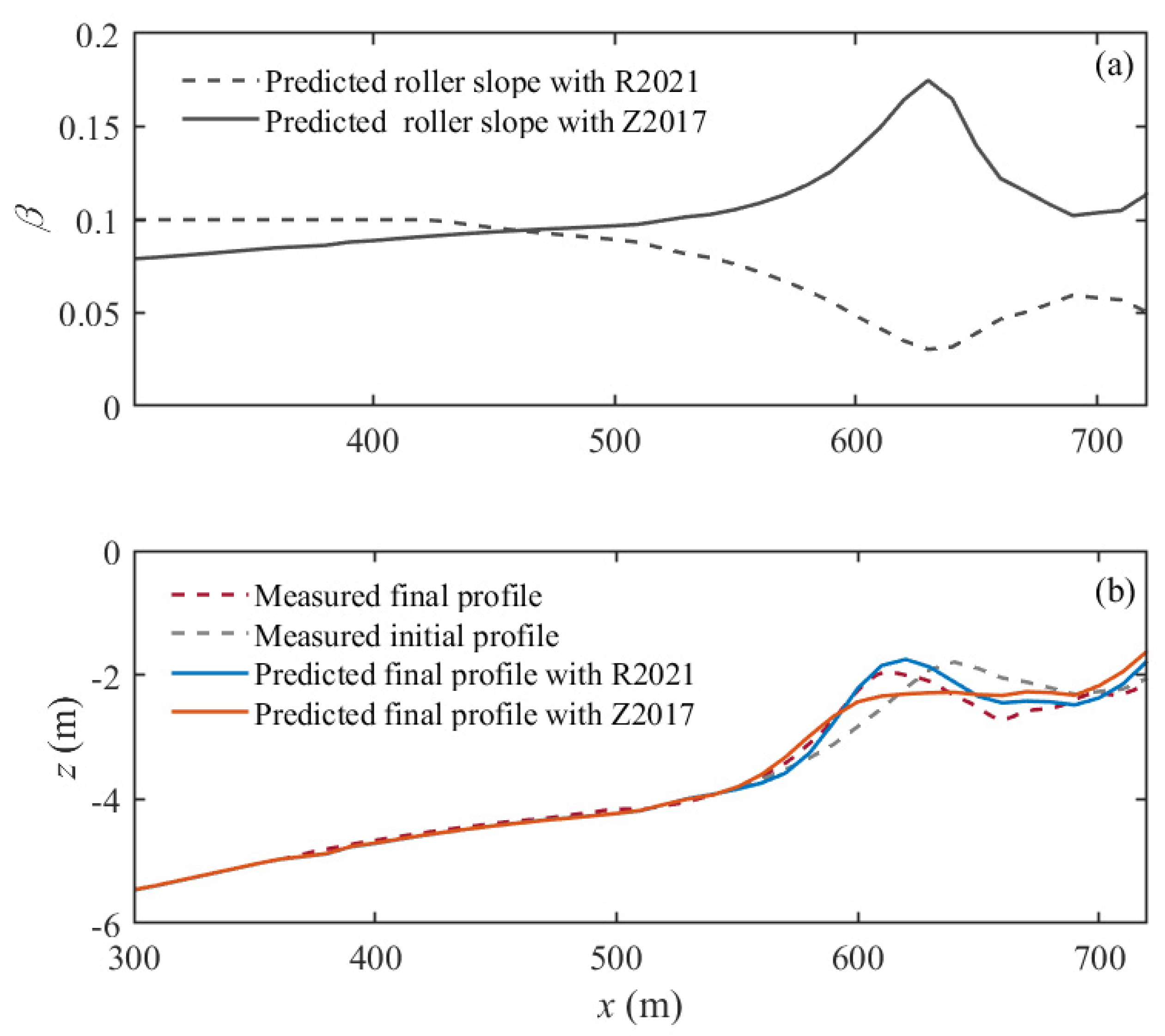
3.2. Model Calibration with Varying Roller Slope

Roller slope formulas in Zhang et al. [22] and Rafati et al. [13] (hereafter, Z2017 and R2021 for brevity) were implemented in the model, while other parameters were unchanged. Please note that this set of parameters is more ‘suitable’ for the constant roller slope since they were calibrated under that assumption. Therefore, it should be taken for granted that the model with the constant roller slope performs better than that with the varying roller slope under this condition. As can be seen in Figure 4a, the roller slope shows a contradictory trend when using Z2017 and R2021. To be specific, Z2017 increases up to the sandbar and then decreases. However, R2021 decreases with the decrease in water depth. Limited by the form of the equation, R2021 cannot capture the increase in the roller slope during wave shoaling. The maximum roller slope of Z2017 was 0.17, located on the sandbar, implying a large roller energy dissipation and weak undertow here. Shoreward of the sandbar, the Z2017 roller slope decreased with an increase in the water depth, achieving a minimum value of 0.1 at the trough of the sandbar. The minimum roller slope of R2021 was 0.03 slightly shoreward of the sandbar; it further increased toward the shoreline. By comparing R2021 and Z2017, the roller slope of R2021 was smaller than that of Z2017 in the inner surf zone, indicating that the R2021 predicted a stronger undertow than Z2017 did.

In Figure 4b, the predicted beach profiles using the model equipped with Z2017 and R2021 are exhibited. The BSSs of profile comparison using Z2017 and R2021 were 0.45 and 0.77, implying a fair fit and a good fit, respectively. The predicted sandbar morphology using Z2017 was less pronounced than that for R2021. This is because R2021 predicts a smaller roller slope and thus a stronger undertow, which can carry suspended sediments from the inner surf zone to reinforce the sandbar [42,43,44,45]. Note that the other model parameters were same as those in the calibration using the constant roller slope. By further tuning other model parameters, the predicted results of Z2017 can be improved. Since we did not attempt to investigate the sensitivity of other model parameters, further model calibration was not conducted here. Although the use of a constant roller slope can obtain an excellent model vs. data comparison, using varying roller slope can also lead to a fair-to-good prediction. The latter, on the other hand, is clearly more physically significant. The main implication of the work is to reduce the calibration parameters in the model and thus to decrease the amount of empirical data required to construct the model.

In the next part, the constant roller slope, as well as the roller slope formulas (i.e., Z2017 and R2021) are implemented in the model to discuss and evaluate the effects of wave height, wave period and sea water level on sediment transport rate and barred beach profile evolution. Six numerical tests were set, as can be seen in

Table 1. Description of numerical cases.

Case ID	Wave Height	Wave Period	Sea Level
1	1.25H0	T0	η0
2	0.8H0	T0	η0
3	H0	1.25T0	η0
4	H0	0.8T0	η0
5	H0	T0	η0 − 10 cm
6	H0	T0	η0 + 10 cm

. Let H₀, T₀ and η₀ be wave heights, wave periods and sea levels in the original case. These values are time-varying rather than constant during the studying period. Case 1 and Case 2 increase or decrease the wave heights to 1.25H₀ or 0.8H₀, with wave periods and sea level unchanged. Case 3 and Case 4 increase or decrease the wave periods to 1.25T₀ or 0.8T₀. The wave parameters of Case 5 and Case 6 are same as the original case, but the sea level is decreased or increased by 10 cm, respectively.

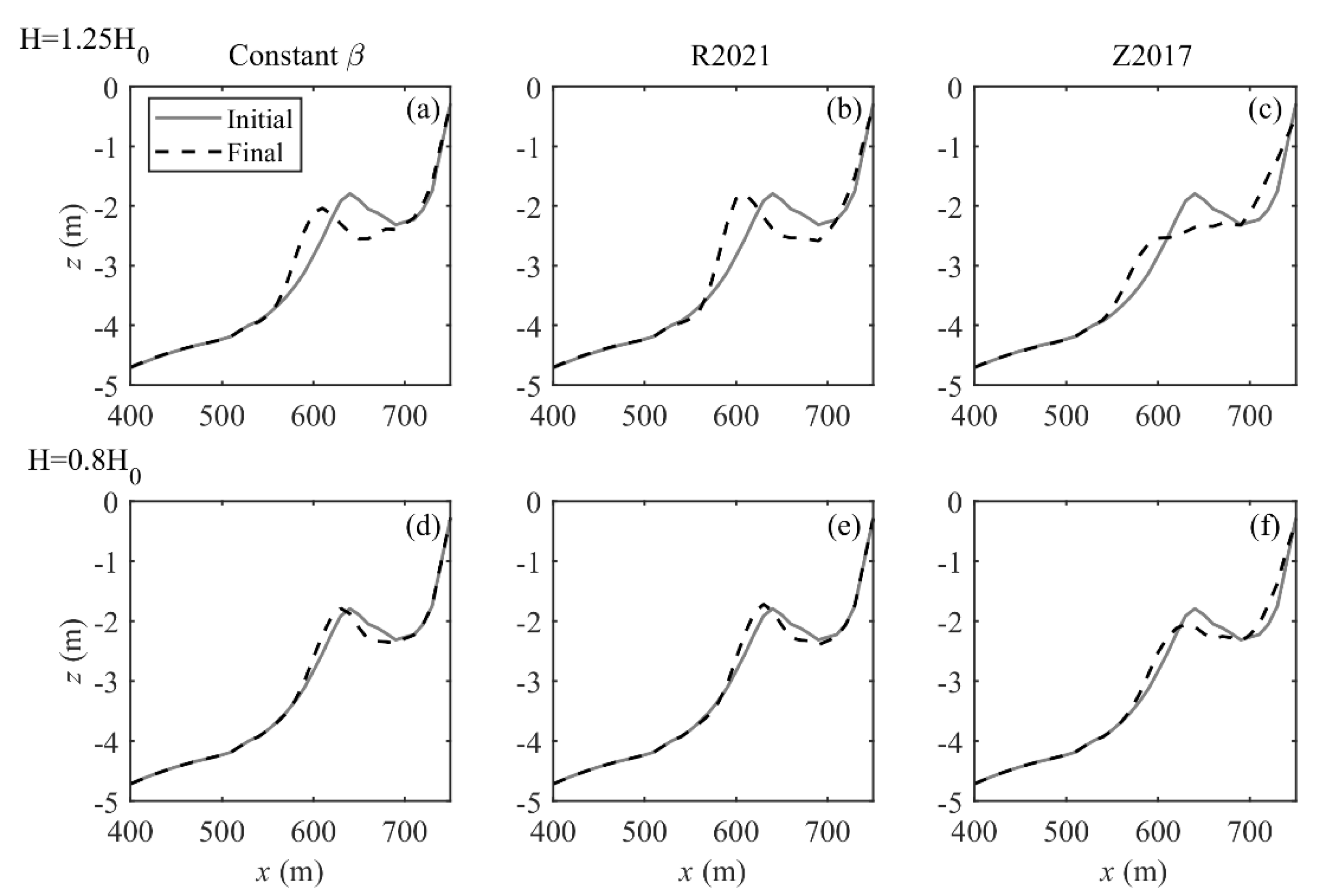
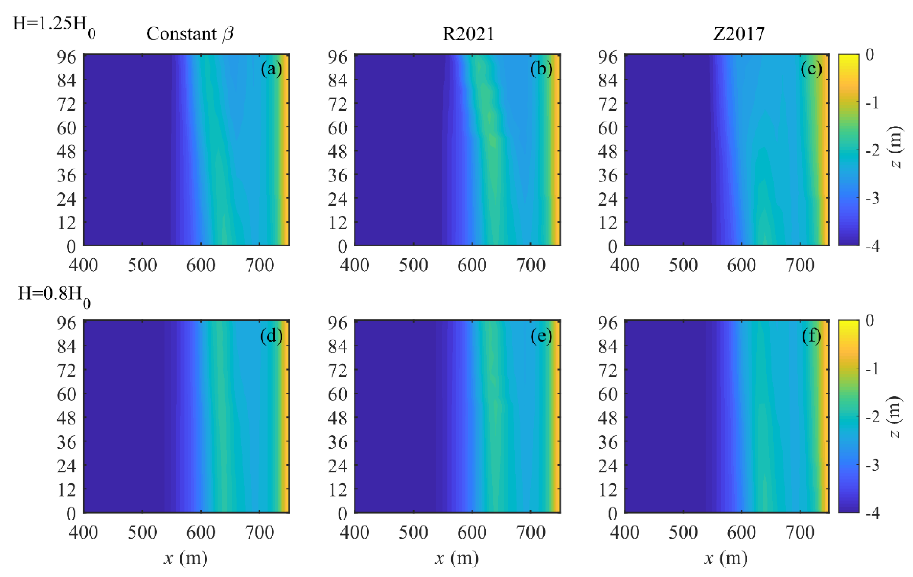
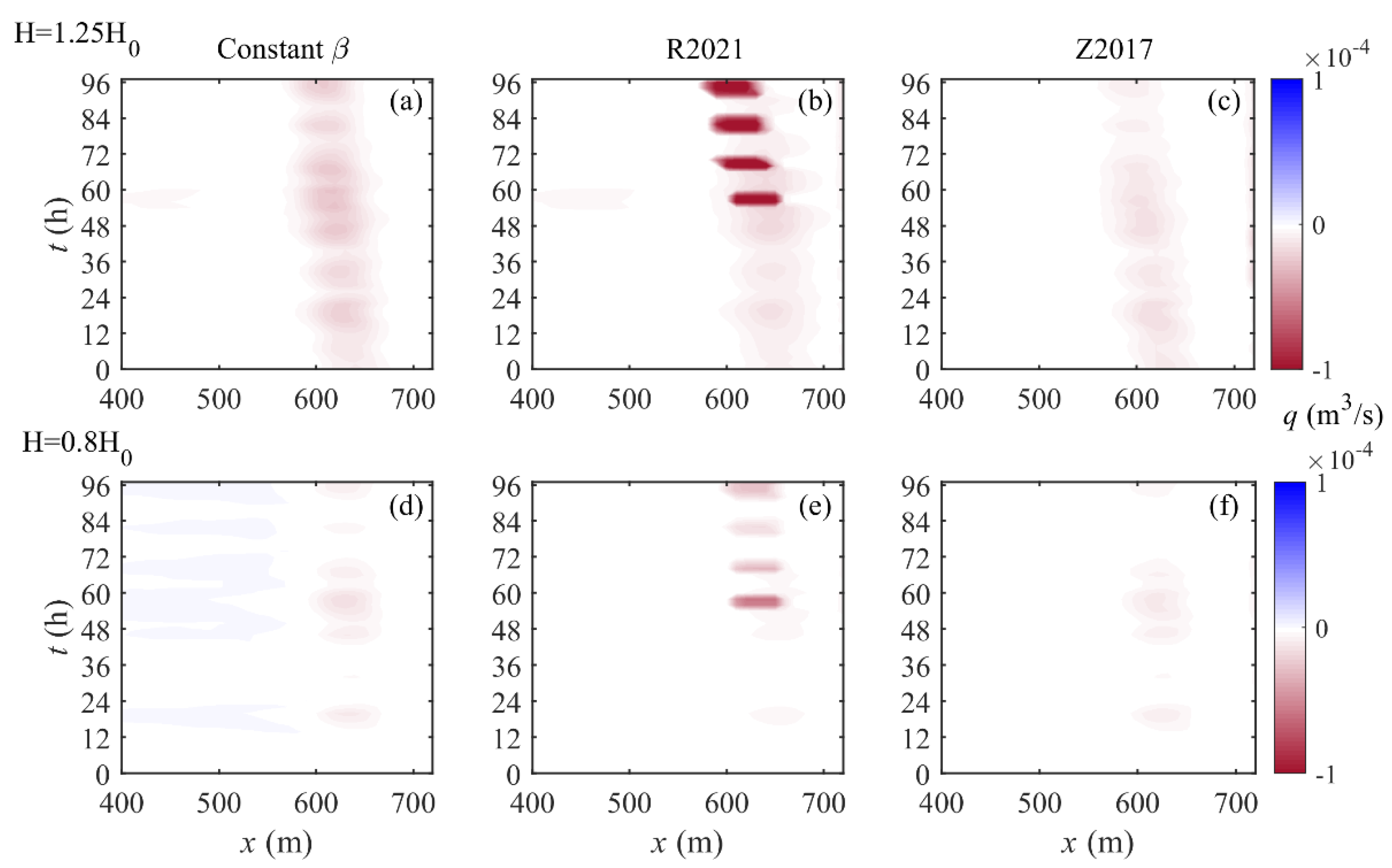
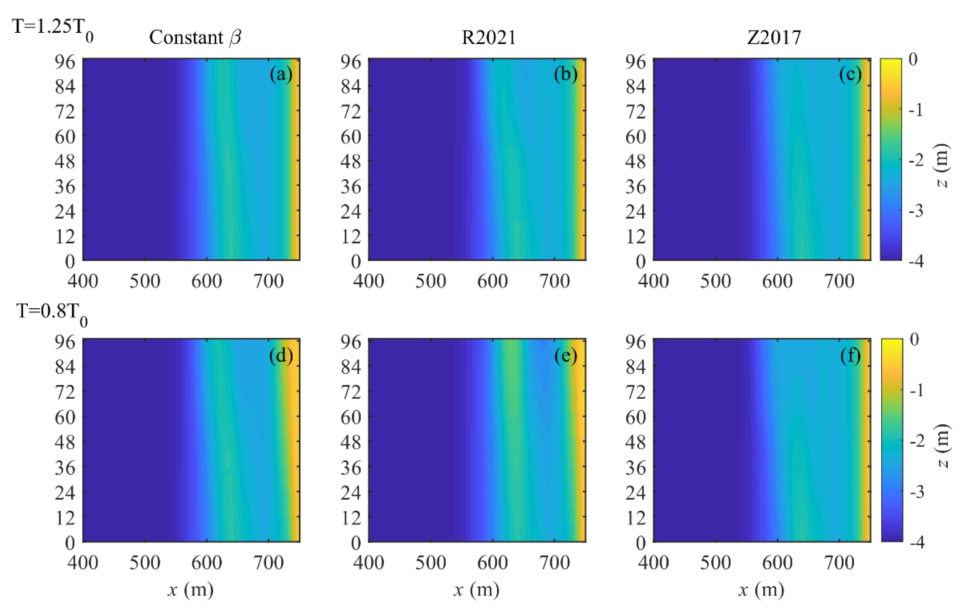
3.3. Effect of Wave Height on Sandbar Evolution

As can be seen in Figure 5, sandbar offshore migration is enhanced when the wave is increased by a factor of 1.25. This is expected because large waves can promote a strong undertow and high sediment concentration in the water column, both of which would facilitate offshore sediment transport and offshore sandbar migration [8,10,11]. However, the CROSPE model implemented with different types of wave roller slopes exhibited varying performance. Using the constant roller slope, as can be seen in Figure 5a,d, the sandbar migrated 40 m offshore and the bar crest elevation decreased by 0.32 m for the larger wave height 1.25H₀, while the sandbar only migrated 10 m offshore and the bar crest elevation remained almost unchanged for the smaller wave height 0.8H₀. By comparing Figure 5a and Figure 5b, using the roller slope formula of R2021 can lead to a more pronounced sandbar. The bar crest elevation either remained unchanged or even increased by 0.07 m, as shown in Figure 5b,c, respectively. When using the roller slope formula of Z2017, the sandbar was found to be more flattened and decaying during its offshore migration. As can be seen in Figure 5c,f, the bar crest elevation decreased by 0.83 m and 0.33 m for Case 1 and 2, respectively. The differences in sandbar migration using R2021 and Z2017 were mainly because R2021 predicted a smaller roller slope shoreward of the sandbar than Z2017 (as provided in Figure 4a and, thus, a larger undertow carrying the sediment offshore to reinforce the sandbar, i.e., to promote a more pronounced sandbar). A large undertow plays an important role in maintaining the shape of the sandbar; this finding has also been discussed [21,42].

Figure 6 provides the spatial–temporal evolution of the sandbar. Using the constant roller slope, the predicted sandbar migrated offshore linearly with time. The offshore migration rates were 10 m/d and 2.5 m/d under wave heights of 1.25H₀ and 0.8H₀, respectively. Using the roller slope formula of R2021 under wave heights of 1.25H₀, the sandbar migrated offshore with a rate of 5 m/d for the first two days, and the migration rate increased to 15 m/d in the following two days, as can be seen in Figure 6b. By comparing Figure 6d and Figure 6c, the predicted sandbar spatial–temporal evolutions under smaller wave height using the constant roller slope and R2021 were similar, although the latter had a more significant bar shape. While using the roller slope formula of Z2017, the bar shape began to decay, and the span of the sandbar increased in the last two days under the larger wave height of 1.25H₀, as can be seen in Figure 6c.

Previous studies show that the main cause of sandbar offshore migration is suspended sediment transport [3,11]. Suspended sediment transport can be further divided into a wave-related component and a current-related component, and the latter is always offshore-directed and mainly controlled by the intensity of the undertow. The depth-integrated and time-averaged suspended sediment transport rate is provided in Figure 7. Under the larger wave height of 1.25H₀, the suspended sediment transport was offshore-directed in the sandbar area and tended to 0 seaward of the sandbar. While under the smaller wave height of 0.8H₀, the magnitude of the suspended sediment transport decreased in the sandbar area and even became positive (i.e., onshore-directed) seaward of the sandbar, as can be seen in Figure 7d. This implies that the current-related component of suspended sediment transport dominates in the sandbar area while the wave-related component dominates seaward of the sandbar. Using the roller slope of R2021 predicts a larger offshore-directed suspended sediment transport rate, i.e., a larger current-related component. It corresponds well with the finding that R2021 predicts a smaller roller slope in the sandbar area and thus a more intense undertow, as can be observed in Figure 7b,e.

Therefore, it can be partly concluded that an increase in wave height can lead to a more rapid and further-offshore migration of the sandbar. Using the roller slope formula of R2021 would predict a larger suspended sediment transport rate in sandbar area, resulting in more sediments being carried to the sandbar to maintain its bar shape. While using the roller slope formula of Z2017 could lead to a weak undertow in sandbar area, resulting in a flattened and decaying bar shape during its offshore migration.

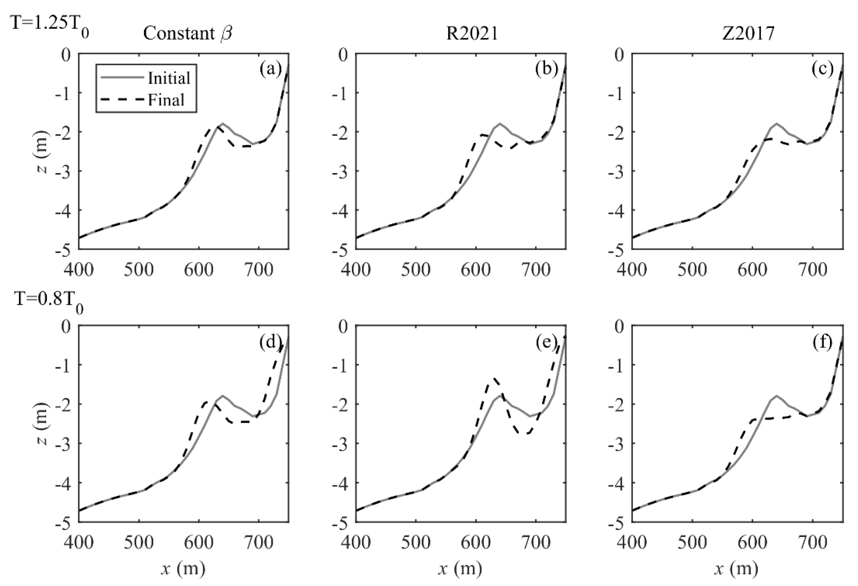
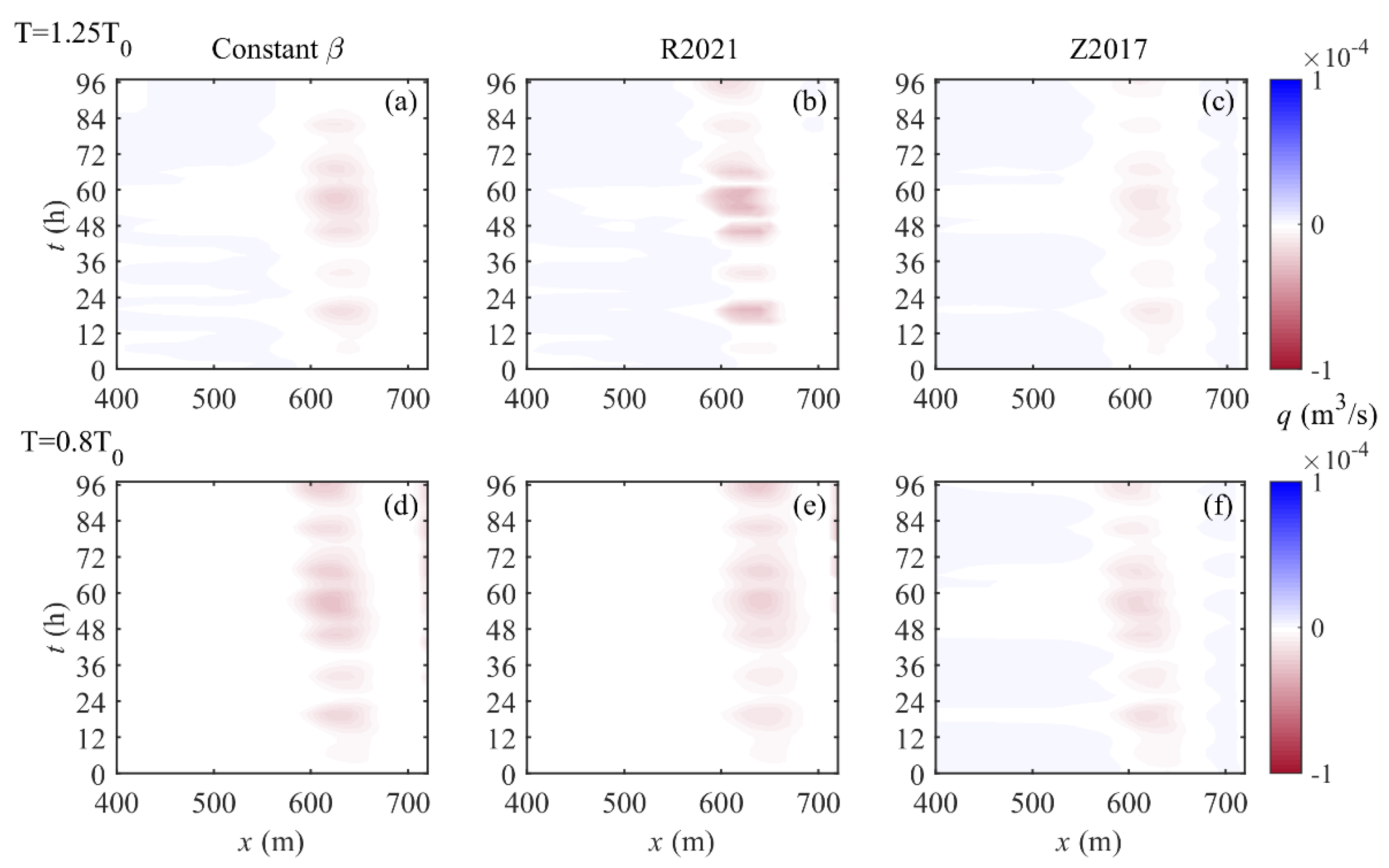
3.4. Effect of Wave Period on Sandbar Migration

As can be seen in Figure 8a,d, the sandbar migrated 20 m and 30 m offshore under the wave period of 1.25T₀ and 0.8T₀, respectively. A decrease in the wave period tends to promote offshore sandbar migration when using the constant roller slope in the model. Although the sandbar was more flattened, the prediction was similar using the roller slope formula of Z2017, the sandbar migrated 30 m and 40 m offshore under the wave period of 1.25T₀ and 0.8T₀, respectively. However, the prediction using R2021 was different. When the wave period decreased, the sandbar became more pronounced, with the bar position remaining almost unchanged.

Similarly, the spatial–temporal evolution of the sandbar under two periods is depicted in Figure 9. As can be seen in Figure 9a,d, the sandbar also migrated offshore linearly with time. The migration rates were 5 m/d and 7.5 m/d, respectively. When using Z2017, the sandbar offshore migration rates increased to 7.5 m/d and 8 m/d under the wave periods of 1.25T₀ and 0.8T₀, respectively. Comparing Figure 9b,c, it can be found that the bar positions were similar when using R2021 and Z2017, but the latter always predicted a more flattened and decaying bar shape.

The sediment transport rates for these two cases are provided in Figure 10. Under the larger wave period 1.25T₀, onshore sediment transport could be observed seaward of the bar crest while the offshore sediment transport occurred shoreward of the bar crest. This is because the wave breaking was weak shoreward of the sandbar because, as can be observed in Figure 3a, the wave height changed insignificantly in this area. Therefore, the undertow was weak, and the wave-related component (caused by the wave nonlinearity) dominated in the area. When the wave period decreased to 0.8T₀, the onshore sediment transport seaward of the sandbar became 0, implying that the quasi-equilibrium was achieved by the wave-related component (onshore) and the undertow-related component (offshore), as can be seen in Figure 10d,e. However, using Z2017 would also predict an onshore sediment transport rate seaward of the sandbar, as can be observed in Figure 10f; it is because Z2017 predicts a larger roller slope and thus a weak undertow, which cannot balance the onshore-directed, wave-related component. It can also be interestingly observed that the position of the offshore sediment transport rate is more shoreward in Figure 10e, i.e., more sediments can be carried from the shore to reinforce the sandbar. Therefore, the sandbar morphology will be more pronounced when using R2021 under the smaller wave period 0.8T₀, as can be seen in Figure 8e and Figure 9e.

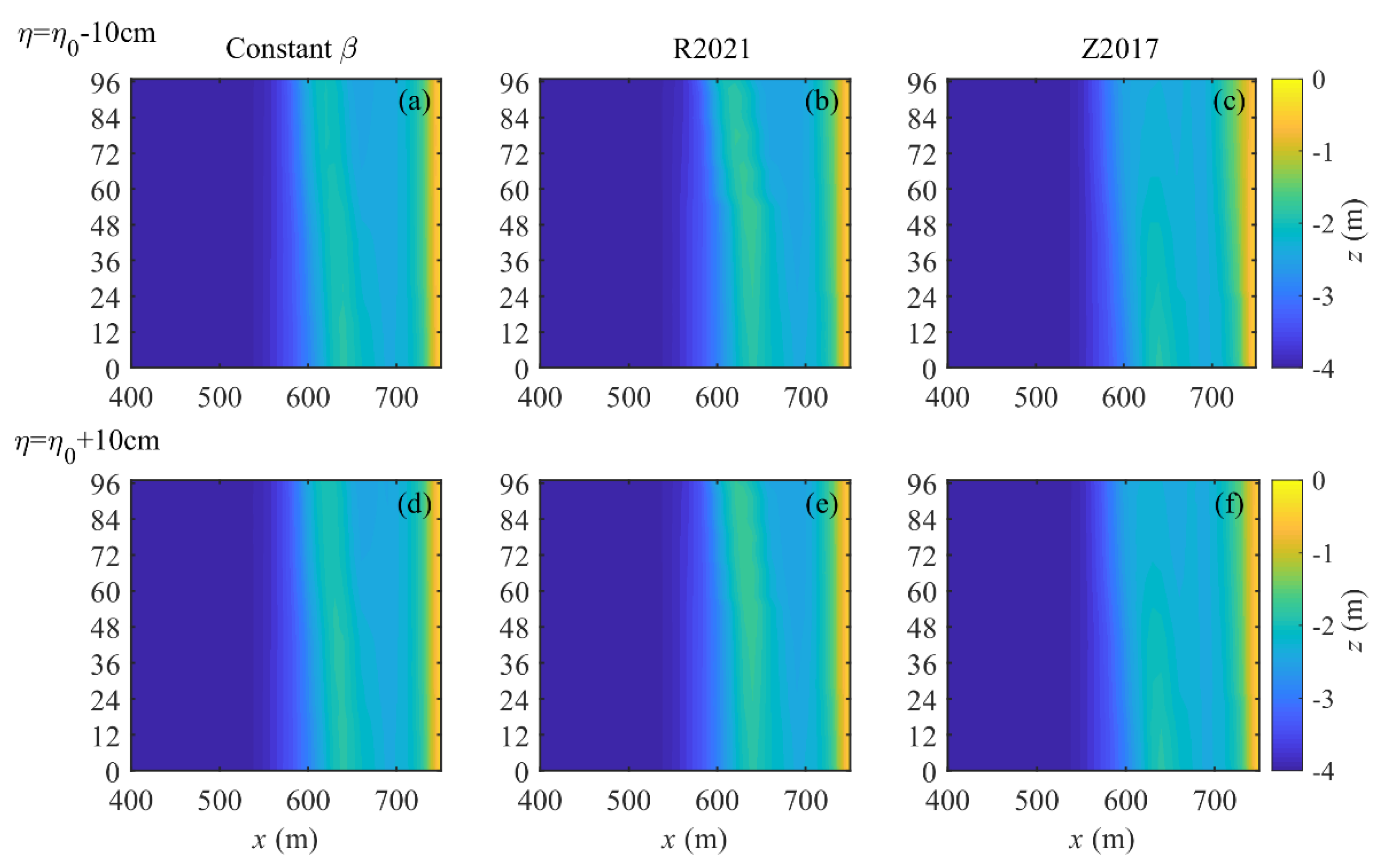
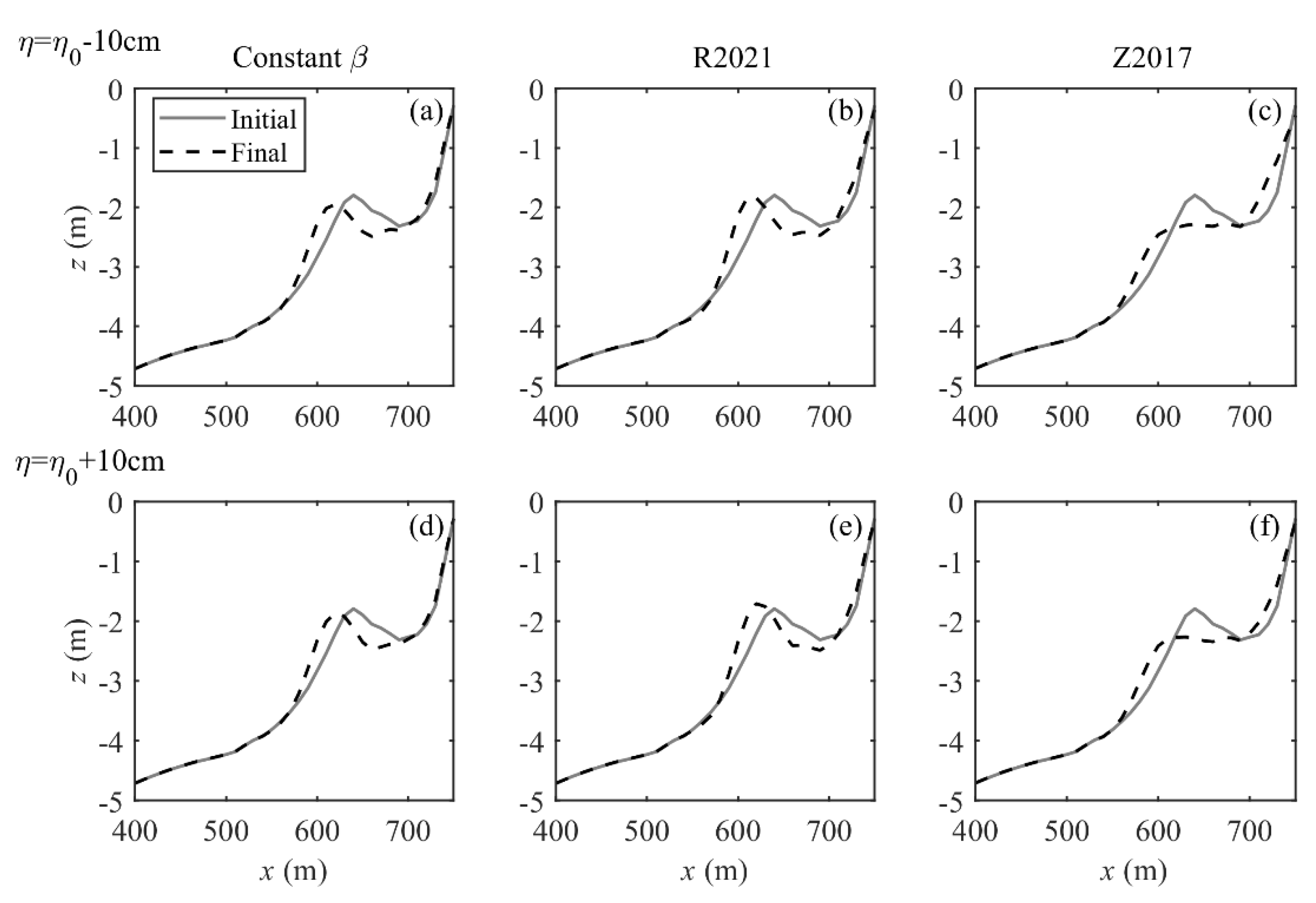
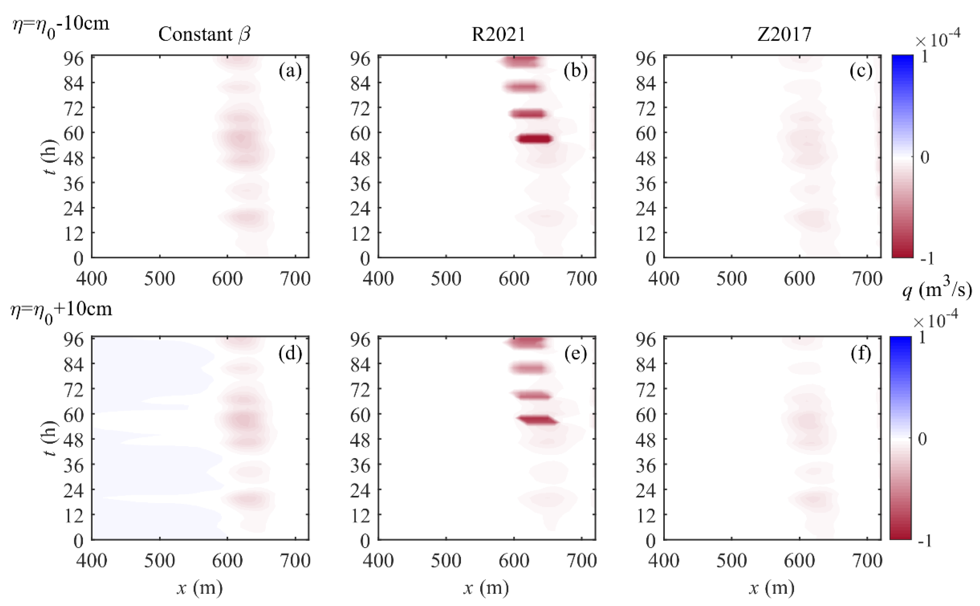
3.5. Effect of Sea Level on Sandbar Migration

As can be seen in Figure 11a,d, the sandbar migration does not show significant variances as the sea level changes. When using the constant roller slope, the bar positions were the same, but the decaying of the bar shape was more obvious for the lower sea level. Except for the insignificant difference in sandbar morphology, the evolutions of the beach face were also different under the two sea levels using the roller slope formulas of R2021 and Z2017. By comparing Figure 11c and Figure 11f, it can be found that the erosion of the beach face increased as the sea level decreased.

Furthermore, the spatial–temporal evolution of the barred beach profile and the suspended sediment transport are provided in Figure 12 and Figure 13, respectively. The sandbar migration rates and suspended sediment transports in the sandbar area were similar under two different sea levels. Although the magnitude of the sediment transport rates was slightly larger under the low sea level than under the high sea level, their trends and positions were similar. This is mainly because the change in sea level was much smaller than the water depth over the sandbar, corresponding to the magnitude of sea level rise on a real-world coast. It can be assumed that the difference in sandbar migration will be enhanced if the sea level variations increase. Future studies will further consider anthropogenic activities that affect sandbar migration, such as beach nourishments, reclamations and harbor constructions [46,47,48].

This study revisited the performance of the roller slope in the beach morphodynamic model. Although Rafati et al. [13] embedded the cross-shore varying roller slope formula in a similar model, XBeach, and proved that the cross-shore varying roller slope worked better than the constant slope in predicting sandbar evolution, we evaluated two different cross-shore varying roller slope formulas that showed different trends that evolve toward the shoreline in this study. Specifically, Z2017 increased to the breaking point (i.e., over the sandbar) and then decreased, implying an unsaturated surf with an obvious wave shoaling process. R2021 generally decreased in the cross-shore direction, indicating a saturated surf. Both the trends of these two formulas are reasonable, and their differences are mainly because they use different calibration datasets. Evaluating these two formulas under changing wave conditions and sea levels in this study can preliminarily illustrate how coastal submerged sandbars will respond to different surf zone conditions (i.e., unsaturated surf zone and saturate surf zone) in future scenarios. Furthermore, the results also have implications on model calibration for predicting the morphological evolution of natural sandbars or shoreface nourishments for future coastal engineering applications [49,50,51].

4. Conclusions

In this study, a process-based numerical model was used to reproduce the barred beach profile evolution in the Duck94 field experiment. The importance of wave roller slope was revisited. Two recent formulas of the roller slope were implemented in the model, and the model results were compared with that using the constant roller slope. Furthermore, six idealized numerical experiments were set to investigate the effect of wave height, wave period and sea level on sandbar migration. The main conclusions are provided below.

By tuning the model parameter, the model using the constant roller slope achieved an excellent performance. Despite this, the model also achieved fair-to-good performances when two recent roller slope formulas were implemented. Under the given circumstances, the varying model parameters clearly make more physical sense, and there is no need to retune the water roller slope parameter.

The roller slope calculated by using R2021 generally decreased with the water depth and usually achieved its minimum at the bar crest. The roller slope calculated by using R2021 increased up to the sandbar crest and then decreased shoreward. Shoreward of the sandbar, the roller slope calculated by using R2021 was smaller than that for Z2017; thus, the predicted sandbar shape was more significant when the model was implemented with R2021. This is because a larger undertow is prone to carry the sediment offshore to reinforce the sandbar.

An increase in the wave height or a decrease in the wave period would lead to a more rapid and further-offshore migration of the sandbar. The offshore-directed, current-related component of suspended sediment transport dominates in the sandbar area, while the onshore-directed, wave-related component is more likely to occur seaward of the sandbar. When the sea level variations are much smaller than the water depth over the sandbar, the effect of sea level change on sandbar migration is negligible; however, a low sea level would cause more erosion on the beach face.

The two roller slope formulas revisited in this study exhibit different trends when evolving to the shoreline. The study is the first to notice and model submerged sandbar evolution using these two roller slope formulas, which represent different surf zone conditions. Based on this study, preliminary insights into the evolution of sandbars in future changing environments are obtained. Future works need to further analyze and optimize model parameters based on measured datasets on near-bottom flow velocity and suspended sediment concentration.

References

1. Cai, F.; Cao, C.; Qi, H.; Su, X.; Lei, G.; Liu, J.; Zhao, S.; Liu, G.; Zhu, K. Rapid Migration of Mainland China’s Coastal Erosion Vulnerability Due to Anthropogenic Changes. J. Environ. Manag. 2022, 319, 115632. [Google Scholar] [CrossRef] [PubMed]
2. Zhang, C.; Zhang, J.; Zheng, J. Coastal Hydrodynamics and Morphodynamics, 2nd ed.; China Communications Press: Beijing, China, 2022. [Google Scholar]
3. Li, Y.; Zhang, C.; Chen, D.; Zheng, J.; Sun, J.; Wang, P. Barred Beach Profile Equilibrium Investigated with a Process-Based Numerical Model. Cont. Shelf Res. 2021, 222, 104432. [Google Scholar] [CrossRef]
4. Wang, P.; Davis, R.A. A Beach Profile Model for a Barred Coast: Case Study from Sand Key, West-Central Florida. J. Coast. Res. 1998, 14, 981–991. [Google Scholar]
5. Jacobsen, N.G.; Fredsøe, J. Cross-Shore Redistribution of Nourished Sand near a Breaker Bar. J. Waterw. Port Coast. Ocean Eng. 2014, 140, 125–134. [Google Scholar] [CrossRef]
6. Lesser, G.; Roelvink, J.; van Kester, J.; Stelling, G. Development and validation of a three-dimensional morphological model. Coast. Eng. 2004, 51, 883–915. [Google Scholar] [CrossRef]
7. Roelvink, D.; Reniers, A.; Van Dongeren, A.; van Thiel De Vries, J.; McCall, R.; Lescinski, J. Modelling storm impacts on beaches, dunes and barrier islands. Coast. Eng. 2009, 56, 1133–1152. [Google Scholar] [CrossRef]
8. Ruessink, G.; Kuriyama, Y.; Reniers, A.; Roelvink, J.A.; Walstra, D.J.R. Modeling cross-shore sandbar behavior on the timescale of weeks. J. Geophys. Res. Atmos. 2007, 112, 1–15. [Google Scholar] [CrossRef] [Green Version]
9. Tong, L.; Liu, P.L.F. Transient Wave-Induced Pore-Water-Pressure and Soil Responses in a Shallow Unsaturated Poroelastic Seabed. J. Fluid Mech. 2022, 938, A36. [Google Scholar] [CrossRef]
10. Zhang, J.; Larson, M. A Numerical Model for Offshore Mound Evolution. J. Mar. Sci. Eng. 2020, 8, 160. [Google Scholar] [CrossRef] [Green Version]
11. Zheng, J.; Zhang, C.; Demirbilek, Z.; Lin, L. Numerical Study of Sandbar Migration under Wave-Undertow Interaction. J. Waterw. Port Coast. Ocean Eng. 2014, 140, 146–159. [Google Scholar] [CrossRef] [Green Version]
12. Reniers, A.; Thornton, E.; Stanton, T.; Roelvink, J. Vertical flow structure during Sandy Duck: Observations and modeling. Coast. Eng. 2004, 51, 237–260. [Google Scholar] [CrossRef]
13. Rafati, Y.; Hsu, T.-J.; Elgar, S.; Raubenheimer, B.; Quataert, E.; van Dongeren, A. Modeling the hydrodynamics and morphodynamics of sandbar migration events. Coast. Eng. 2021, 166, 103885. [Google Scholar] [CrossRef]
14. Walstra, D.J.R.; Mocke, G.P.; Smit, F. Roller Contributions as Inferred from Inverse Modelling Techniques. In Coastal Engineering Proceedings; Amer Society of Civil Engineers: Orlando, FL, USA, 1996; pp. 1205–1218. [Google Scholar]
15. Wang, A.; Wu, X.; Bi, N.; Ralston, D.K.; Wang, C.; Wang, H. Combined Effects of Waves and Tides on Bottom Sediment Resuspension in the Southern Yellow Sea. Mar. Geol. 2022, 452, 106892. [Google Scholar] [CrossRef]
16. Zhang, Y.; Hong, X.; Qiu, T.; Liu, X.; Sun, Y.; Xu, G. Tidal and wave modulation of rip current dynamics. Cont. Shelf Res. 2022, 243, 104764. [Google Scholar] [CrossRef]
17. Chi, S.-H.; Zhang, C.; Sui, T.-T.; Cao, Z.-B.; Zheng, J.-H.; Fan, J.-S. Field observation of wave overtopping at sea dike using shore-based video images. J. Hydrodyn. 2021, 33, 657–672. [Google Scholar] [CrossRef]
18. Zhang, J.; Larson, M.; Ge, Z.P. Numerical Model of Beach Profile Evolution in the Nearshore. J. Coast. Res. 2020, 36, 506. [Google Scholar] [CrossRef]
19. Pan, Y.; Yin, S.; Chen, Y.P.; Yang, Y.B.; Xu, C.Y.; Xu, Z.S. An experimental study on the evolution of a submerged berm under the effects of regular waves in low-energy conditions. Coast. Eng. 2022, 176, 104169. [Google Scholar] [CrossRef]
20. Li, Y.; Zhang, C.; Cai, Y.; Xie, M.; Qi, H.; Wang, Y. Wave Dissipation and Sediment Transport Patterns during Shoreface Nourishment towards Equilibrium. J. Mar. Sci. Eng. 2021, 9, 535. [Google Scholar] [CrossRef]
21. Li, Y.; Zhang, C.; Dai, W.; Chen, D.; Sui, T.; Xie, M.; Chen, S. Laboratory investigation on morphology response of submerged artificial sandbar and its impact on beach evolution under storm wave condition. Mar. Geol. 2021, 443, 106668. [Google Scholar] [CrossRef]
22. Zhang, C.; Zhang, Q.; Zheng, J.; Demirbilek, Z. Parameterization of nearshore wave front slope. Coast. Eng. 2017, 127, 80–87. [Google Scholar] [CrossRef]
23. Zhang, C.; Li, Y.; Zheng, J.; Xie, M.; Shi, J.; Wang, G. Parametric modelling of nearshore wave reflection. Coast. Eng. 2021, 169, 103978. [Google Scholar] [CrossRef]
24. Baldock, T.E.; Holmes, P.; Bunker, S.; Van Weert, P. Cross-Shore Hydrodynamics within an Unsaturated Surf Zone. Coast. Eng. 1998, 34, 173–196. [Google Scholar] [CrossRef]
25. Thornton, E.B.; Guza, R.T. Transformation of Wave Height Distribution. J. Geophys. Res. 1983, 88, 5925–5938. [Google Scholar] [CrossRef] [Green Version]
26. Janssen, T.T.; Battjes, J.A. A Note on Wave Energy Dissipation over Steep Beaches. Coast. Eng. 2007, 54, 711–716. [Google Scholar] [CrossRef]
27. Zhang, C.; Li, Y.; Cai, Y.; Shi, J.; Zheng, J.; Cai, F.; Qi, H. Parameterization of Nearshore Wave Breaker Index. Coast. Eng. 2021, 168, 103914. [Google Scholar] [CrossRef]
28. Apotsos, A.; Raubenheimer, B.; Elgar, S.; Guza, R.T.; Smith, J.A. Effects of wave rollers and bottom stress on wave setup. J. Geophys. Res. 2007, 112, C02003. [Google Scholar] [CrossRef] [Green Version]
29. Dally, W.R.; Brown, C.A. A modelling investigation of the breaking wave roller with application to cross-shore currents. J. Geophys. Res. 1995, 100, 24873–24883. [Google Scholar] [CrossRef]
30. Dong, G.; Chen, H.; Ma, Y. Parameterization of Nonlinear Shallow Water Waves over Sloping Bottoms. Coast. Eng. 2014, 94, 23–32. [Google Scholar] [CrossRef]
31. Li, Y.; Zhang, C.; Chen, S.; Sui, T.; Chen, D.; Qi, H. Influence of Artificial Sandbar on Nonlinear Wave Transformation: Experimental Investigation and Parameterizations. Ocean Eng. 2022, 257, 111540. [Google Scholar] [CrossRef]
32. Zheng, J.; Yao, Y.; Chen, S.; Chen, S.; Zhang, Q. Laboratory study on wave-induced setup and wave-driven current in a 2DH reef-lagoon-channel system. Coast. Eng. 2020, 162, 103772. [Google Scholar] [CrossRef]
33. Feddersen, F.; Guza, R.T.; Elgar, S.; Herbers, T.H.C. Alongshore momentum balances in the nearshore. J. Geophys. Res. Ocean. 1998, 103, 15667–15676. [Google Scholar] [CrossRef]
34. Gallagher, E.L.; Elgar, S.; Guza, R.T. Observations of Sand Bar Evolution on a Natural Beach. J. Geophys. Res. Ocean. 1998, 103, 3203–3215. [Google Scholar] [CrossRef] [Green Version]
35. Long, C.E. Index and Bulk Parameters for Frequency-Direction Spectra Measured at CERC Field Research Facility, June 1994 to August 1995. Misc. Pap. CERC-96-6. 1996. Available online: https://onlinebooks.library.upenn.edu/webbin/book/lookupid?key=ha102348778 (accessed on 10 November 2021).
36. Zhang, J.; Larson, M. Decadal-Scale Subaerial Beach and Dune Evolution at Duck, North Carolina. Mar. Geol. 2021, 440, 106576. [Google Scholar] [CrossRef]
37. Li, Y.; Zhang, C.; Chi, S.-H.; Yang, Y.-H.; Shi, J.; Sui, T.-T. Numerical test of scale relations for modelling coastal sandbar migration and inspiration to physical model design. J. Hydrodyn. 2022, 34, 700–711. [Google Scholar] [CrossRef]
38. Zhao, S.H.; Cai, F.; Qi, H.S.; Zhu, J.; Zhou, X.; Lei, G.; Zheng, J.X. Contrasting sand-mud transition migrations of estuarine and bay beaches and their potential morphological responses. Geomorphology 2020, 365, 107243. [Google Scholar] [CrossRef]
39. Zhao, S.H.; Qi, H.S.; Cai, F.; Zhu, J.; Zhou, X.; Lei, G. Morphological and sedimentary features of sandy-muddy transitional beaches in estuaries and bays along mesotidal to macrotidal coasts. Earth Surf. Process. Landf. 2020, 45, 1660–1676. [Google Scholar] [CrossRef]
40. van Rijn, L.C.; Walstra, D.J.R.; Grasmeijer, B.; Sutherland, J.; Pan, S.; Sierra, J. The predictability of cross-shore bed evolution of sandy beaches at the time scale of storms and seasons using process-based profile models. Coast. Eng. 2003, 47, 295–327. [Google Scholar] [CrossRef]
41. Roelvink, J.A.; Stive, M.J.F. Bar-Generating Cross-Shore Flow Mechanisms on a Beach. J. Geophys. Res. Ocean. 1989, 94, 4785–4800. [Google Scholar] [CrossRef]
42. Sanchez-Arcilla, A.; Caceres, I. An Analysis of Nearshore Profile and Bar Development under Large Scale Erosive and Accretive Waves. J. Hydraul. Res. 2017, 56, 231–244. [Google Scholar] [CrossRef]
43. Kuang, C.; Mao, X.; Gu, J.; Niu, H.; Ma, Y.; Yang, Y.; Qiu, R.; Zhang, J. Morphological processes of two artificial submerged shore-parallel sandbars for beach nourishment in a nearshore zone. Ocean Coast. Manag. 2019, 179, 104870. [Google Scholar] [CrossRef]
44. Kuang, C.; Ma, Y.; Han, X.; Pan, S.; Zhu, L. Experimental Observation on Beach Evolution Process with Presence of Artificial Submerged Sand Bar and Reef. J. Mar. Sci. Eng. 2020, 8, 1019. [Google Scholar] [CrossRef]
45. Kuang, C.; Han, X.; Zhang, J.; Zou, Q.; Dong, B. Morphodynamic Evolution of a Nourished Beach with Artificial Sandbars: Field Observations and Numerical Modeling. J. Mar. Sci. Eng. 2021, 9, 245. [Google Scholar] [CrossRef]
46. Gao, J.; Ma, X.; Zang, J.; Dong, G.; Ma, X.; Zhu, Y.; Zhou, L. Numerical investigation of harbor oscillations induced by focused transient wave groups. Coast. Eng. 2020, 158, 103670. [Google Scholar] [CrossRef]
47. Gao, J.; Ma, X.; Dong, G.; Chen, H.; Liu, Q.; Zang, J. Investigation on the effects of Bragg reflection on harbor oscillations. Coast. Eng. 2021, 170, 103977. [Google Scholar] [CrossRef]
48. Zhao, S.; Cai, F.; Liu, Z.; Cao, C.; Qi, H. Disturbed Climate Changes Preserved in Terrigenous Sediments Associated with Anthropogenic Activities During the Last Century in the Taiwan Strait, East Asia. Mar. Geol. 2021, 437, 106499. [Google Scholar] [CrossRef]
49. Shafiei, H.; Chauchat, J.; Bonamy, C.; Marchesiello, P. Adaptation of the Santoss Transport Formula for 3d Nearshore Models: Application to Cross-Shore Sandbar Migration. Ocean Model. 2022, 181, 102138. [Google Scholar] [CrossRef]
50. Marchesiello, P.; Chauchat, J.; Shafiei, H.; Almar, R.; Benshila, R.; Dumas, F.; Debreu, L. 3D wave-resolving simulation of sandbar migration. Ocean Model. 2022, 180, 102127. [Google Scholar] [CrossRef]
51. Fang, K.; Yi, F.; Liu, J.; Sun, J. Laboratory study on the effect of an artificial sandbar on nourished beach profile evolution. Int. J. Offshore Polar Eng. 2022, 32, 218–226. [Google Scholar] [CrossRef]
Figure 1. Research area and the location of the Field Research Facility.
Water 15 00923 g001
Figure 2. Time series of (a) RMS wave height; (b) wave peak period; (c) wave angle; (d) water level; (e) measured initial and final profiles.
Water 15 00923 g002
Figure 3. Comparison of (a) RMS wave height and (b) beach profile using a constant roller slope of 0.08.
Water 15 00923 g003
Figure 4. Comparisons of (a) roller slope and (b) beach profile evolution by using Z2017 and R2021.
Water 15 00923 g004
Figure 5. Comparisons of beach profile predicted by constant roller slope (a,d), roller slope of R2021 (b,e) and Z2017 (c,f) under two different wave heights. Figure 5a–c are calculated with H = 1.25H0, and Figure 5d–f are calculated with H = 0.8H0.
Water 15 00923 g005
Figure 6. Spatial–temporal evolution of the sandbar predicted by constant roller slope (a,d) and the roller slope of R2021 (b,e) and Z2017 (c,f) under two different wave heights. Figure 6a–c are calculated with H = 1.25H0, and Figure 6d–f are calculated with H = 0.8H0.
Water 15 00923 g006
Figure 7. Spatial–temporal evolution of the suspended sediment transport rate predicted by constant roller slope (a,d) and the roller slope of R2021 (b,e) and Z2017 (c,f) under two different wave heights. Figure 7a–c are calculated with H = 1.25H0, and Figure 7d–f are calculated with H = 0.8H0.
Water 15 00923 g007
Figure 8. Comparisons of beach profile predicted by constant roller slope (a,d) and the roller slope of R2021 (b,e) and Z2017 (c,f) under two different wave periods. Figure 8a–c are calculated with T = 1.25T0, and Figure 8d–f are calculated with T = 0.8T0.
Water 15 00923 g008
Figure 9. Spatial–temporal evolution of the sandbar predicted by constant roller slope (a,d) and the roller slope of R2021 (b,e) and Z2017 (c,f) under two different wave periods. Figure 9a–c are calculated with T = 1.25T0, and Figure 9d–f are calculated with T = 0.8T0.
Water 15 00923 g009
Figure 10. Spatial–temporal evolution of the suspended sediment transport rate predicted by constant roller slope (a,d) and the roller slope of R2021 (b,e) and Z2017 (c,f) under two different wave periods. Figure 10a–c are calculated with T = 1.25T0, and Figure 10d–f are calculated with T = 0.8T0.
Water 15 00923 g010
Figure 11. Comparisons of beach profile predicted by constant roller slope (a,d) and the roller slope of R2021 (b,e) and Z2017 (c,f) under two different sea levels. Figure 11a–c are calculated with η0 − 10 cm, and Figure 11d–f are calculated with η0 + 10 cm.
Water 15 00923 g011
Figure 12. Spatial–temporal evolution of the sandbar predicted by constant roller slope (a,d) and the roller slope of R2021 (b,e) and Z2017 (c,f) under two different sea levels. Figure 12a–c are calculated with η0 − 10 cm, and Figure 12d–f are calculated with η0 + 10 cm.
Water 15 00923 g012
Figure 13. Spatial–temporal evolution of the suspended sediment transport rate predicted by constant roller slope (a,d) and the roller slope of R2021 (b,e) and Z2017 (c,f) under two different sea levels. Figure 13a–c are calculated with η0 − 10 cm, and Figure 13d–f are calculated with η0 + 10 cm.
Water 15 00923 g013