Research on Sustainable Scheduling of Cascade Reservoirs Based on Improved Crow Search Algorithm

Abstract

As an important tool for the development and utilization of river water conservancy and hydropower resources, cascade reservoirs will directly affect human life and ecological environment. Therefore, how to sustainably and rationally dispatch the water resources of cascade reservoirs is of great importance to human society and ecological environment. In order to solve this problem, this paper constructs the objective function by considering the three goals of reservoir power generation target, social benefit and ecological benefit. On this basis, a mathematical model of cascade reservoir scheduling is established considering multi-dimensional constraints such as water transmission and water supply capacity constraints, water level constraints and flow constraints. In addition, we consider the fact that the crow search algorithm (CSA) is easy to fall into as the local optimal solution due to the influence of its flight distance parameters on the search ability when solving large-scale optimization problems. Therefore, a crow search algorithm based on particle swarm optimization (PSO-CSA) is designed to solve the multi-objective scheduling model of cascade reservoir established in this paper. Finally, this paper compares the PSO-CSA algorithm, PSO algorithm, CSA algorithm and genetic algorithm (GA) which is widely used in reservoir water resource dispatch, through a simulation example. The simulation results show the superiority of the algorithm designed in this paper in solving the water resource control problem of cascade reservoirs.

1. Introduction

Water is very important to the entire human society, and how to rationally use water resources has always been the focus of relevant researchers [1]. A cascade reservoir uses the cascade development method to develop the river, and build the reservoir along the river section by section, so as to make more reasonable use of the river’s water resources. This method leads to a cascade arrangement of a series of reservoirs along the river from upstream to downstream, which is why it is named cascade reservoir [2]. Figure 1 shows the major cascade reservoirs of the State Water Project (SWP) in California, USA. SWP collects water from rivers in Northern California and distributes the collected water resources to the water supply areas in Southern California and San Francisco Bay Area through the cascade reservoir system [3].

The water resource dispatch of cascade reservoirs, as an important means of river water runoff regulation, directly affects the water shortage of the regional water supply system and the power generation of the reservoir [4]. In addition, the lack of water in the water supply system will have an impact on the surrounding ecological environment and residential water use. Therefore, the goal of using only a single objective function for the water resource dispatch of cascade reservoirs is no longer applicable, and it is urgent to propose a multi-objective scheduling method for cascade reservoirs to meet the needs of cascade reservoir scheduling [5].

At this stage, reservoir optimization scheduling and cascade reservoir scheduling are mostly carried out in the background of flood control [5,6,7,8]. Ahmad, A. et al. [9] establish a single-objective mathematical model based on the water resource scheduling for agricultural irrigation, and studied single reservoir scheduling based on meta-heuristic algorithms to reduce the agricultural water supply deficit of the reservoir. Similarly, Bashiri-Atrabi, H. et al. [10] designed a single-objective mathematical model for the scheduling of a single reservoir. On this basis, the optimization of a multi-reservoir hydropower system is studied. This study establishes a single-objective mathematical model to maximize the generation of cascade reservoirs [11]. Bozorg-Haddad, O. et al. [12] study the multi-objective optimization of cascade reservoirs, focusing on reducing pollution and water supply deficit. In addition, a two-objective mathematical model focusing on the maximization of energy production and the minimization of water supply deficit has been established [13].

When dealing with multi-objective optimization problems, with the development of swarm intelligence technology, a large number of algorithms have emerged in recent years [14,15]. An improved genetic algorithm is designed to solve multi-objective optimization problems [16]. Similarly, Recio et al. designed a particle-swarm-based genetic algorithm based on genetic algorithms to solve reservoir multi-objective scheduling problems. It can be seen that algorithms including differential evolution algorithms and genetic algorithms are widely used in multi-objective optimization problems [17]. As a novel bio-inspired algorithm, the CSA algorithm has the advantages of simple structure and fewer parameters, and has been gradually applied to multi-objective optimization problems [18].

As for the relevant algorithms of reservoir scheduling, genetic algorithm (GA), as a representative technology in the field of evolutionary computing, has been widely used in reservoir scheduling problems [1,8]. Rashid et al. [19] and Babamiri, O. et al. [20] both designed genetic algorithms to solve the reservoir scheduling problem. In addition, an improved sine–cosine algorithm is designed to solve the reservoir scheduling problem [21]. The simulation results show that the algorithm has excellent performance in solving the reservoir scheduling problem. Seifollahi-Aghmiuni, S. et al. [22] apply the improved evolutionary algorithm to the reservoir scheduling problem, and achieve good results, providing a certain reference for the improvement of the heuristic algorithm. Based on the theory of swarm intelligence, an improved heuristic algorithm was designed for the scheduling model of hydropower stations [23]. Chen et al. designed an improved PSO algorithm for reservoir flood control scheduling tasks. Experimental results show that compared with the GA algorithm, the improved PSO algorithm has a better effect in dealing with reservoir scheduling problems [24].

In addition, the issue of reservoir dispatch in the context of hydropower generation has also received extensive attention from relevant researchers. According to the characteristics of the reservoir power generation system, Ford et al. established a multi-reservoir-based co-generation model. Experimental results show that this scheme plays an important role in reducing costs and improving efficiency in hydropower generation [25]. Sakthivel et al. [26] optimized power generation by optimizing water flow. Acuña et al. [27] designed corresponding models and algorithms to improve the capacity of hydropower plants. Zhang et al. [28] considered the ecological indicators on the basis of considering the power generation indicators, so as to establish the corresponding mathematical model and carry out the research of reservoir scheduling, which has a certain reference significance for this paper.

It can be seen from the above studies that cascade reservoir dispatch research for flood control and power generation purposes has been widely available. However, there are certain gaps in the research on sustainable cascade reservoir scheduling for daily use, industrial water and ecological water. In view of this problem, in order to make reasonable use of the water resources of cascade reservoirs, the ecological water demand objective is introduced into the mathematical model, and the corresponding constraints are improved. This paper establishes a multi-objective function model with the smallest industrial, agricultural, ecological and living water shortage rates with the largest power generation capacity of the reservoirs. Further, according to the multi-objective function model, the corresponding solution algorithm is designed to form a sustainable cascade reservoir scheduling scheme. This scheme enables the reservoir to solve the contradiction of the water resource demands of industry, agriculture and domestic use, and avoid harm to the ecological environment around the reservoir while ensuring the goal of reservoir power generation.

The rest of this paper is structured as follows: The second part of the article reviews the relevant research on optimal reservoir scheduling at this stage. The third part of the paper establishes a multi-objective mathematical model of cascade reservoirs. In the fourth part of the article, an algorithm is proposed. The fifth part of the article conducts simulation experiments. Finally, the conclusions are given in the sixth part.

2. Multi-Objective Sustainable Scheduling Model of Cascade Reservoirs

2.1. Problem Description

Figure 2 shows the topology of cascade reservoirs in the Oroville–Thermalito Complex. The Oroville–Thermalito Complex belongs to the California State Water Project, which is composed of a cascade reservoir system and is the source of SWP. The maximum capacity of the Oroville–Thermalito Complex is 4.47 Km³. Lake Oroville reservoir (hereafter referred to as reservoir A) is the upstream reservoir of the cascade reservoir system; Thermolito Forebay reservoir (hereafter referred to as reservoir B) is a downstream reservoir; Thermolito Afterbay reservoir (hereafter referred to as reservoir C) is located at the end of reservoir B, and the length of the canal connecting reservoir B and reservoir C is only 2.8 km. Reservoir A, reservoir B and reservoir C jointly form the Oroville–Thermalito Complex.

It can be seen from Figure 2 that during the scheduling of the cascade reservoir system, reservoir A has inflow runoff to supply water; reservoir A carries water by gravity to reservoir B; reservoir B can carry water by gravity to reservoir C, and reservoir C can also carry water from reservoir A through the lifting water station. During the scheduling of the cascade reservoir system, reservoir A is responsible for replenishing water to reservoir B and reservoir C, and supplying water to water supply area I. The water in water supply area I can be divided into four parts: industrial water, agricultural water, ecological water and domestic water. Reservoir B is responsible for replenishing water to reservoir C and supplying water to water supply area II. Taking one year as a decision-making cycle and one month as a time period, the joint sustainable scheduling of the A-B-C cascade is to determine the discharge flow of each reservoir during the month based on the inflow of reservoir A and the power generation index, water supply index, etc., of reservoir A, reservoir B and reservoir C.

It is worth pointing out that when solving a multi-objective mathematical model, whether it is a Pareto solution or other solution, and then making a decision, it is inevitable that it will be influenced by expert experience. Therefore, the mathematical model established in this paper is as follows.

2.2. Model Establishment

Before establishing the model, this paper first gives some symbolic descriptions, as shown in

Table 1. Symbol Description.

Symbol	Illustrate
$\Delta t$	The duration of the unit period
$T$	scheduling period set, $T=\left\{1,2,\cdot \cdot \cdot ,t\right\}$
$N$	Reservoir set, $N=\left\{1,2,\cdot \cdot \cdot ,n\right\}$
$L_{n,t,U}$	The upstream water level $n$ of the reservoir during the time period $t$
$L_{n,t,D}$	The downstream level $n$ of the reservoir during the time period $t$
$L_{n,t,L}$	Loss of head $n$ of reservoirs within time $t$
$Q_{t,n,G}$	The flow rate of generators in reservoir $n$ within the time period $t$
$Q_{t,n,G\max }$	The maximum flow rate of generators in reservoir $n$ in the time period $t$
$Q_{t,P}^n$	The discharge rate of the reservoir $n$
$Q_{t,I}^n$	The flow rate of the reservoir $n$
${\overline{Q}}_{n-1,n}$	The three-year average runoff within the $n-1\to n$ river section
$Q_{t,R,I}^{n-1,n}$	The water demand of industry within the time period $t$ of the $n-1\to n$ river section
$Q_{t,R,A}^{n-1,n}$	The water demand of agriculture within the time period $t$ of the $n-1\to n$ river section
$Q_{t,R,D}^{n-1,n}$	The water demand of residents during the time period $t$ of the $n-1\to n$ river section
$Q_{t,R,E}^{n-1,n}$	The water demand of the ecological environment during the time period $t$ of the $n-1\to n$ river section
$Q_{t,P,I}^{n-1,n}$	The amount of water provided by industry in the river section during the time period $t$ of the $n-1\to n$ river section
$Q_{t,P,A}^{n-1,n}$	The amount of water provided by agriculture in the river section during the time period $t$ of the $n-1\to n$ river section
$Q_{t,P,D}^{n-1,n}$	The amount of water provided by residents in the river section during the time period $t$ of the $n-1\to n$ river section
$Q_{t,P,E}^{n-1,n}$	The amount of water provided of the ecological environment during the time period $t$ in the $n-1\to n$ river section
${\xi }_{t,L}^{n-1,n}$	Water scarcity indicator function during the time period $t$ within a river section $n-1\to n$
${\xi }_{t,L,E}^{n-1,n}$	Water shortage index function of ecological environment during the time period $t$ in the river section $n-1\to n$
${\delta }_n$	The output coefficient of the generator of the reservoir $n$

.

According to the goal of sustainable operation of cascade reservoirs in this paper, the multi-objective functions of maximizing power generation, minimizing water shortage in agriculture, industry and domestic, and minimizing water shortage in ecological environment are established as follows.

$$\min f={\displaystyle \sum _{n\in N}{\displaystyle \sum _{t\in T}{\xi }_{t,L}^{n-1,n}}}\times {\displaystyle \sum _{n\in N}{\displaystyle \sum _{t\in T}{\xi }_{t,L,E}^{n-1,n}}}\times \frac{1}{{\displaystyle \sum _{t\in T}{\displaystyle \sum _{n\in N}\left(Q_{t,n,G}\times {\delta }_n\times \Delta H_n\times \Delta t\right)}}}$$

(1)

Among them, the calculation formula of the reservoir power generation is $Q_{t,n,G}\times {\delta }_n\times \Delta H_n\times \Delta t$. That is, the product of the passing flow, power generation time, head and generator output coefficient. The calculation method of the water shortage index function ${\xi }_{t,L}^{n-1,n}$ and ${\xi }_{t,L,E}^{n-1,n}$ the water shortage index function of the ecological environment in the time period $t$ of the river section $n-1\to n$ is shown in Formulas (2) and (3). The head $\Delta H_n$ of the reservoir $n$ is calculated as shown in Equation (4).

$${\xi }_{t,L}^{n-1,n}={\omega }_i\times \frac{\left(Q_{t,R,I}^{n-1,n}-Q_{t,P,I}^{n-1,n}\right)}{Q_{t,R,I}^{n-1,n}}+{\omega }_a\times \frac{\left(Q_{t,R,A}^{n-1,n}-Q_{t,P,A}^{n-1,n}\right)}{Q_{t,R,A}^{n-1,n}}+{\omega }_d\frac{\left(Q_{t,R,D}^{n-1,n}-Q_{t,P,D}^{n-1,n}\right)}{Q_{t,R,D}^{n-1,n}}$$

(2)

Among them, ${\omega }_i$ is the weight coefficient of industrial water shortage rate, ${\omega }_a$ is the weight coefficient of the agricultural water shortage rate, ${\omega }_d$ is the weight coefficient of the water shortage rate of residents. The three coefficients are determined based on expert experience, and the specific relationship is shown in Equation (5).

$${\xi }_{t,L,E}^{n-1,n}=\frac{\left(Q_{t,R,E}^{n-1,n}-Q_{t,P,E}^{n-1,n}\right)}{Q_{t,R,E}^{n-1,n}}$$

(3)

$$\Delta H_n=L_{n,t,U}-L_{n,t,D}-L_{n,t,L}$$

(4)

The specific calculation method of $\Delta H_n$ is the water level in the upstream section of reservoir $n$ minus the water level in the downstream section of reservoir $n$, minus the head loss of reservoir $n$.

$${\omega }_i+{\omega }_a+{\omega }_d=1$$

(5)

On this basis, the following constraints are established according to the structure of the reservoir and the relevant performance indicators.

Minimum ecological water constraints

$$Q_{t,R,E}^{n-1,n}\ge \zeta \times {\overline{Q}}_{n-1,n}$$

(6)

Constraint (6) guarantees a minimum limit for ecological water use, where $\zeta$ is the ecological water use coefficient. Generally, 10% of the average runoff of the river within the time period $t$ is taken. This constraint further ensures the sustainability of water dispatch in cascade reservoirs.

Reservoir maximum and minimum water level constraints

$$L_{n\min }\le L_{n,t}\le L_{n\max }$$

(7)

$$L_{n,t}=\frac{Q_{t,I}^n-Q_{t,P}^n}{S_n}+L_{n,t-1}$$

(8)

Constraints (7) and (8) constrain the highest and lowest water levels of reservoir $n$ in the time period $t$. Among them, the actual water level of the reservoir $n$ in the $L_{n,t}$ period $t$; $L_{n\min },L_{n\max }$ are the highest and lowest water levels of the reservoir $n$ in the time period $t$, respectively. Equation (8) is how $n$ is calculated. Where $S_n$ is the cross-sectional area of the reservoir.

Reservoir water balance constraints

$$Vo{l}_{t,n}=Vo{l}_{t-1,n}+\left(Q_{t,I}^n-Q_{t,P}^n\right)\times \Delta t-Q_{t,n,L}$$

(9)

Constraint (9) ensures the balance of the number of reservoirs, that is, the amount of water entering the reservoir minus the amount of water out minus the loss of water and the original water volume of the reservoir is equal to the existing quantity of the reservoir. Where $Q_{t,n,L}$ is the water loss of the reservoir $n$ in the time period $t$, including the number of infiltration, the amount of evaporation, etc.

Constraints of maximum flow through the turbine of reservoir power station

$$Q_{t,n,G}\le Q_{t,n,G\max }$$

(10)

Formula (10) ensures that the flow through the turbine of the reservoir power station does not exceed its maximum flow rate.

The above constraints ensure the timing constraints such as the stagnant water level, the highest water level and the maximum outflow of the reservoir, which provides a basis for the practical application of the model established in this paper.

3. PSO-CSA Algorithm Design

3.1. Introduction to the Algorithm

As a novel bio-inspired algorithm, CSA algorithm has been widely used in the field of optimization. LIU et al. [18] and Razavi et al. [29] both explore the application of a CSA algorithm to multi-objective optimization problems, and the study of the above problems provides theoretical support for the application of CSA algorithm in reservoir scheduling problems.

The CSA algorithm was proposed by Askarzadeh et al. in 2016 inspired by the foraging behavior of crows in nature. During the foraging process, crows will hide excess food in a hidden location and choose a suitable time to remove it. An interesting phenomenon is that in the crow population, each individual crow is very greedy and will follow each other, and once crow A gets the location of the food hidden by another crow, crow A will steal from him at the right time. In addition, when the tracked crow finds itself being followed, the tracked crow will try to run to another place as a way to confuse the stalker. Therefore, the CSA algorithm follows the following principles:

• Multiple crow individuals form crow populations and live as populations.
• Each individual crow can remember where he or she hides their food.
• The crows in the crow population will find and steal each other’s food by tracking.
• When an individual crow being followed discovers that it is being followed, it takes steps to confuse the other party.
• Specifically, the specific process of the CSA algorithm is as follows:

Step 1. Initialize the problem parameters. Initialization parameters include the population capacity $P$ of the crow population; maximum number of iterations ${\lambda }_{\max }$; raven flight length $\psi$; crow perception probability $\varphi$; the dimension of the problem $D$.

Step 2. Initialize the location and memory of crows in the crow population.

$$C_{rp}=\left[\begin{array}{cccc}{c}_1^1& c_2^1& \cdots & c_d^1\\ c_1^2& c_2^2& \cdots & c_d^2\\ ⋮& ⋮& ⋮& ⋮\\ c_1^P& c_2^P& \cdots & c_d^P\end{array}\right]$$

(11)

$$c^{p,\lambda }=\left[c_1^{p,\lambda },c_2^{p,\lambda },\cdot \cdot \cdot ,c_d^{p,\lambda }\right],p\in P$$

(12)

Among them, Equation (11) is the initialization formula for the position of individual crows in the crow population; in Equation (12), $c^{p,\lambda }$ is the position vector of crow $p$ during the $\lambda$ iteration.

$$Mc=\left[\begin{array}{cccc}{m}_1^1& m_2^1& \cdots & m_d^1\\ m_1^2& m_2^2& \cdots & m_d^2\\ ⋮& ⋮& ⋮& ⋮\\ m_1^P& m_2^P& \cdots & m_d^P\end{array}\right]$$

(13)

Among them, Equation (13) is the memory initialization formula of individual crows in the crow population.

Step 3. Calculate the fitness function. According to the objective function formula, the fitness function value of each crow’s position is calculated from the position vector of that crow.

Step 4. Update the position of crows in the crow population as shown in Equation (14).

$$c^{p,\lambda +1}=\{\begin{array}{c}{c}^{p,\lambda }+ran{d}_1\left(h\right)\times {\psi }^{p,\lambda }\times \left(m^{h,\lambda }-c^{p,\lambda }\right),\hspace{1em}ran{d}_1\left(h\right)\ge {\varphi }^{h,\lambda }\\ Random Position,\hspace{1em}Others\end{array}$$

(14)

Among them, the crow $p$ updates its position by tracking the crow $h$, and if the crow $h$ does not know that it is being tracked, the position of the crow $p$ is updated according to the $ran{d}_1\left(h\right)\ge {\varphi }^{h,\lambda }$ time in Formula (14). Where $ran{d}_1\left(h\right)$ is a random number in the interval (0, 1); ${\varphi }^{h,\lambda }$ is the perceived probability of crow $h$ during the $\lambda$ iteration. If Raven $h$ knows that he is being tracked, the position of raven $p$ is updated as “Others” in Equation (14).

Step 5. Detect the feasibility of a new location for crow $p$. If the crow’s new position satisfies the constraints of the problem, the crow updates the position; if the crow’s new location does not meet the constraints of the question, the location update is not made. Calculate the new fitness function value based on the updated position of the crow $p$.

Step 6. Update the memory of the crow, and determine whether to update the memory of the crow through the fitness function value of the crow’s new position, the specific formula is as follows.

$$m^{p,\lambda +1}=\{\begin{array}{c}{c}^{p,\lambda +1},\hspace{1em}f\left(c^{p,\lambda +1}\right)\le f\left(m^{p,\lambda +1}\right)\\ m^{p,\lambda +1},\hspace{1em}Others\end{array}$$

(15)

Step 7. Determine whether the maximum number of iterations ${\lambda }_{\max }$ has been reached, and output the result if so, otherwise return Step 4 to repeat the operation.

3.2. Improvement Strategy

Because the CSA algorithm is in the solution process, when the crow finds that there are other crows tracking it, the update randomness of the crow position is too high, which is conducive to the algorithm jumping out of the local optimal solution, but it also causes the convergence accuracy of the algorithm to be low. In addition, the update of the crow’s memory, because the update formula is too simple, is not conducive to algorithm optimization. Therefore, the CSA algorithm is not ideal for dealing with large-scale problems such as reservoir scheduling, so the PSO algorithm is combined with the CSA algorithm, and the feeding strategy of whales is introduced, and a new hybrid algorithm is designed to solve the problem.

3.2.1. The Crow Flies at Variable Speed

Since the crow search algorithm performs position updates, the flight speed is a fixed value. Therefore, the crow variable speed flight strategy is designed to imitate the update method of particle velocity in the particle swarm, as shown in Equation (16).

$${\psi }^{p,\lambda +1}={\psi }^{p,\lambda }+\beta \times ran{d}_2\times \left(\min \left(c^{p^{\prime },\lambda }\right)-c^{p,\lambda }\right)$$

(16)

where $\beta$ is the learning factor; $ran{d}_2$ is a random number in the interval (0, 1); $\min \left(c^{p^{\prime },\lambda }\right)$ is the position of the individual with the best fitness function produced by the individual crow in the current number of iterations.

3.2.2. Raven Spiral Update Location Strategy

In order to increase the choice of crow position update, the crow spiral update position strategy is designed. The position of the crow is updated based on the distance between the stalker and the tracked individual in the crow population. Raven $p$ updates its position by tracking raven $h$, and if raven $h$ does not know that it is being tracked, raven $p$‘s position is updated according to $ran{d}_1\left(h\right)\ge {\varphi }^{h,\lambda }$ in Equation (17). If raven $h$ knows that they are being followed, the position of raven $p$ is updated as in the case of $ran{d}_1\left(h\right)<{\varphi }^{h,\lambda }$ in Equation (18).

$$c^{p,\lambda +1}=\{\begin{array}{c}{c}^{p,\lambda }+ran{d}_1\left(h\right)\times {\psi }^{p,\lambda }\times \left(m^{h,\lambda }-c^{p,\lambda }\right),\hspace{1em}ran{d}_1\left(h\right)\ge {\varphi }^{h,\lambda }\\ c^{p,\lambda +1}\ast ,\hspace{1em}ran{d}_1\left(h\right)<{\varphi }^{h,\lambda }\end{array}$$

(17)

$$c^{p,\lambda +1}\ast =\{\begin{array}{c}{l}^{\rightharpoonup }\times e^{b\times ran{d}_3}\times \cos \left(2\pi ran{d}_3\right)+c^{p,\lambda },\hspace{1em}ran{d}_3\le 0.5\\ Random Position,\hspace{1em}ran{d}_3>0.5\end{array}$$

(18)

In Equation (19), $l^{\rightharpoonup }$ is the distance between crow $h$ and crow $p$, and the specific calculation formula is shown in Equation (19). $b$ is a helical shape constant; $ran{d}_3$ is a random number in the interval (0, 1).

$$l^{\rightharpoonup }=\left|c^{p,\lambda }-c^{h,\lambda }\right|$$

(19)

3.2.3. Crow Memory Contraction Update Strategy

In order to increase the choice of crow memory update, this paper designs a crow memory contraction update strategy according to the whale’s contraction encirclement strategy. The fitness function value of the crow’s new position is used to determine whether to update the crow’s memory. There are three main update methods, as shown in Formulas (20) and (21).

$$m^{p,\lambda +1}=\{\begin{array}{cc}{c}^{p,\lambda +1},& f\left(c^{p,\lambda +1}\right)\le f\left(m^{p,\lambda +1}\right)\\ m^{p,\lambda +1}\ast ,& f\left(c^{p,\lambda +1}\right)>f\left(m^{p,\lambda +1}\right)\end{array}$$

(20)

$$m^{p,\lambda +1}\ast =\{\begin{array}{c}{c}^{p,\lambda +1}-ran{d}_4\times \mu \times l^{\rightharpoonup },\hspace{1em}ran{d}_4\le 0.5\\ m^{p,\lambda },\hspace{1em}ran{d}_4>0.5\end{array}$$

(21)

where $ran{d}_4$ is a random number in the interval (0, 1), $\mu$ is the memory contraction coefficient. When the fitness function relationship is $f\left(c^{p,\lambda +1}\right)\le f\left(m^{p,\lambda +1}\right)$, the $\lambda +1$ memory $m^{p,\lambda +1}$ of the generation of crow $p$ is updated to the position of the $\lambda +1$ generation of crow $p$. When the fitness function relationship is $f\left(c^{p,\lambda +1}\right)>f\left(m^{p,\lambda +1}\right)$, the memory $m^{p,\lambda +1}$ of the $\lambda +1$ generation of crow $p$ is updated according to the Formula (21) update. First, a random number $ran{d}_4$ is generated, and when $ran{d}_4\le 0.5$, the memory $m^{p,\lambda +1}$ of the $\lambda +1$ generation of crow $p$ is updated according to the crow memory contraction update strategy; when $ran{d}_4>0.5$, the memory $m^{p,\lambda +1}$ of the $\lambda +1$ generation of the crow $p$ keeps the memory of the previous generation unchanged.

3.3. Improve the Specific Solution Steps of the Algorithm

Step 1. Initialize problem parameters such as decision variables in the reservoir scheduling model. Initialization parameters include the population capacity $P$ of the crow population; maximum number of iterations ${\lambda }_{\max }$; crow flight length $\psi$; crow perception probability $\varphi$; the dimension of the problem $D$; memory contraction coefficient $\mu$; helical shape constant $b$; learning factor $\beta$.

Step 2. Initialize the location and memory of crows in the crow population.

Step 3. The fitness function is calculated according to Equation (1).

Step 4. Update the crow’s flight length according to the crow’s variable speed flight strategy. This is shown in Equation (17).

Step 5. Update crow positions in the crow population according to the spiral update location strategy. This is shown in Equations (18) and (19).

Among them, the crow $p$ updates its position by tracking the crow $h$, and if the crow $h$ does not know that it is being tracked, the position of the crow $p$ is updated according to the $ran{d}_1\left(h\right)\ge {\varphi }^{h,\lambda }$ in Formula (18). If raven $h$ knows that it is being tracked, the position of raven $p$ is updated as $ran{d}_1\left(h\right)<{\varphi }^{h,\lambda }$ case in Equation (19).

Step 6. Detect the feasibility of a new location for a crow. If the crow’s new position satisfies the constraints of the problem, the crow updates the position; if the crow’s new location does not meet the constraints of the question, the location update is not made. Calculate the new fitness function value based on the updated position of the crow $p$.

Step 7. Update the crow’s memory, and determine whether to update the crow’s memory by the fitness function value of the crow’s new position, as shown in Formulas (21) and (22).

Among them, the memory $m^{p,\lambda +1}$ update strategy of the $\lambda +1$ generation of crow $p$ is: when the fitness function relationship is $f\left(c^{p,\lambda +1}\right)\le f\left(m^{p,\lambda +1}\right)$, update to the position of the $\lambda +1$ generation of crow $p$. When $ran{d}_4\le 0.5\wedge f\left(c^{p,\lambda +1}\right)>f\left(m^{p,\lambda +1}\right)$, update according to the crow memory contraction update strategy; when $ran{d}_4>0.5\wedge f\left(c^{p,\lambda +1}\right)>f\left(m^{p,\lambda +1}\right)$, the crow’s memory remains unchanged from the previous generation.

Step 8. Determine whether the maximum number of iterations ${\lambda }_{\max }$ is reached, and if so, output the scheduling result of cascade reservoir water resources, otherwise return to Step 4 to repeat the operation.

4. Results and Discussion

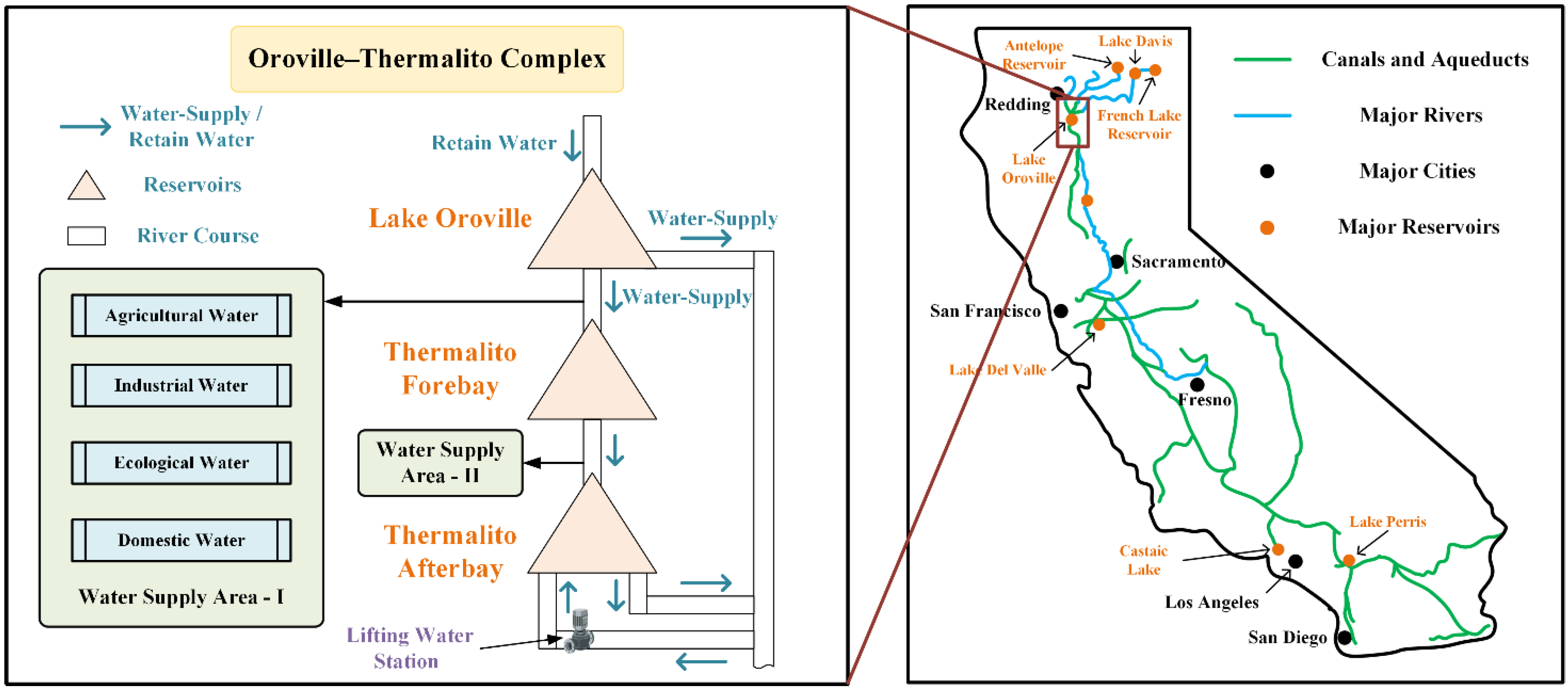
4.1. Overview of Engineering Background

In order to further demonstrate the effect of the model established in this paper and the algorithm in the sustainable scheduling problem of cascade reservoirs, this paper selects the Lake Oroville Reservoir (reservoir A) and its adjacent downstream reservoir, the Thermalito Forebay Reservoir (reservoir B), which belong to the Oroville-Thermalito Complex, for dispatch when the incoming flow is known. Lake Oroville Reservoir is a large reservoir located in the California waterways, the main source of water in the California waterways, and is a reservoir for water storage, power generation, flood control, tourism, and comprehensive utilization of fish and wildlife, with an installed capacity of 644,000 kW and six generator sets, three of which are pumped storage units for power generation and pumping, with a reservoir capacity of 4.36$\times {10}^8$ m³.

The water demand of industry, agriculture, residents’ living and ecological environment in the unit period of reservoir A and reservoir B in December in a certain year are shown in

Table 2. Water demand from reservoir A and reservoir B over different periods of time.

Month		1	2	3	4	5	6	Total
Reservoir	Purpose	$\mathbf{Water} \mathbf{Demand} (\mathbf{Unit}:\times {\mathbf{10}}^{\mathbf{4}}{\mathbf{m}}^{\mathbf{3}})$
A	Industry	1000	1012	1224	1200	1200	1500
	Agriculture	509	500	2400	3972	4675	5825
	Domestic	85	90	90	100	115	115
	Ecology	75	88	90	115	167	199
B	Industry	750	780	795	795	740	800
	Agriculture	240	250	709	771	895	950
	Domestic	600	590	580	625	707	794
	Ecology	133	135	139	180	188	195
Month		7	8	9	10	11	12
Reservoir	Purpose	Water Demand (Unit:$\mathbf{\times }{\mathbf{10}}^{\mathbf{4}}$m3)
A	Industry	1400	1500	1224	1200	1000	1344	14,804
	Agriculture	5990	4614	1200	1150	504	300	31,641
	Domestic	120	140	140	122	95	95	1307
	Ecology	204	207	200	188	152	107	1792
B	Industry	820	950	890	825	825	755	9725
	Agriculture	945	900	864	752	400	295	7972
	Domestic	790	787	746	690	605	610	8124
	Ecology	199	195	180	172	150	145	2011

.

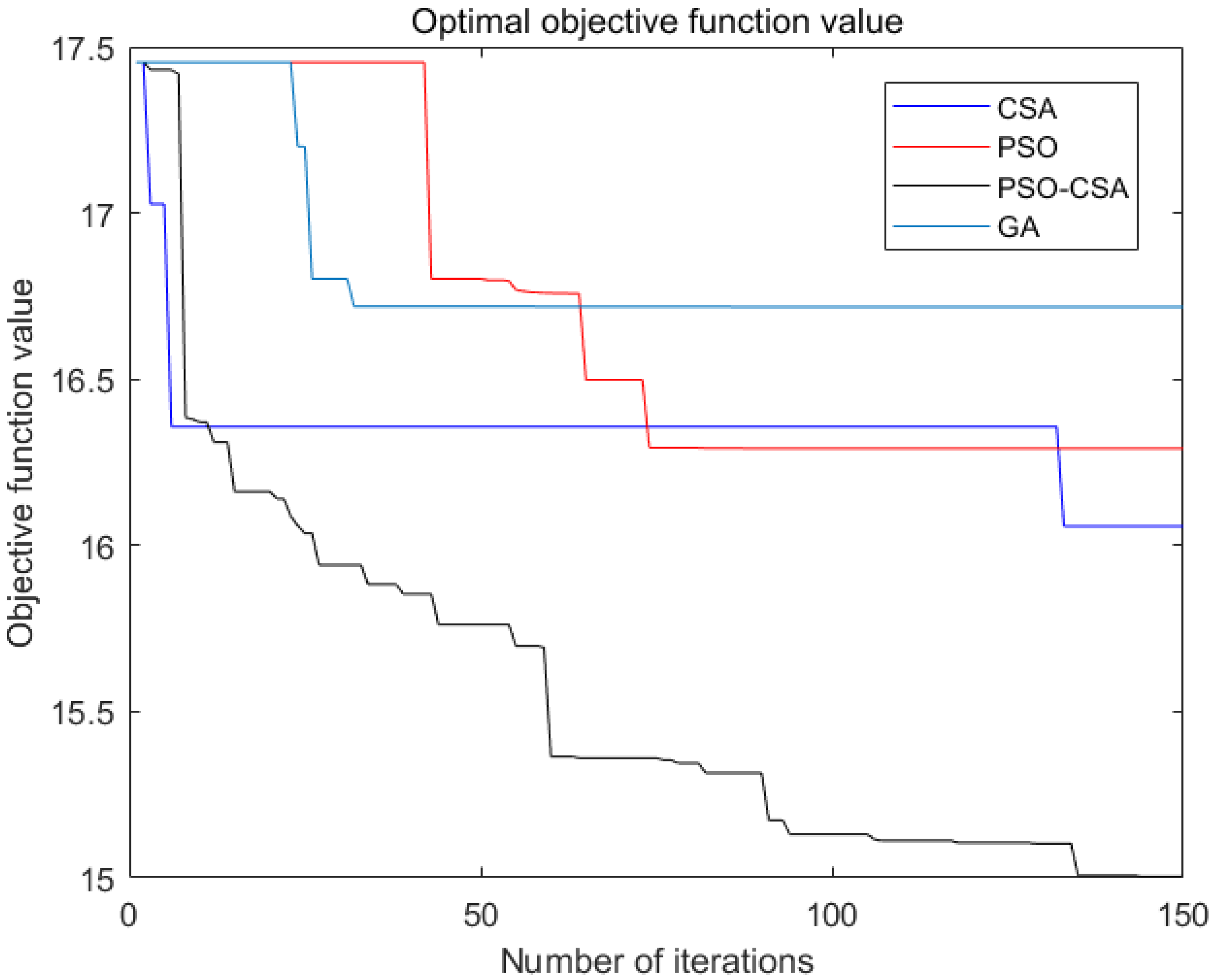
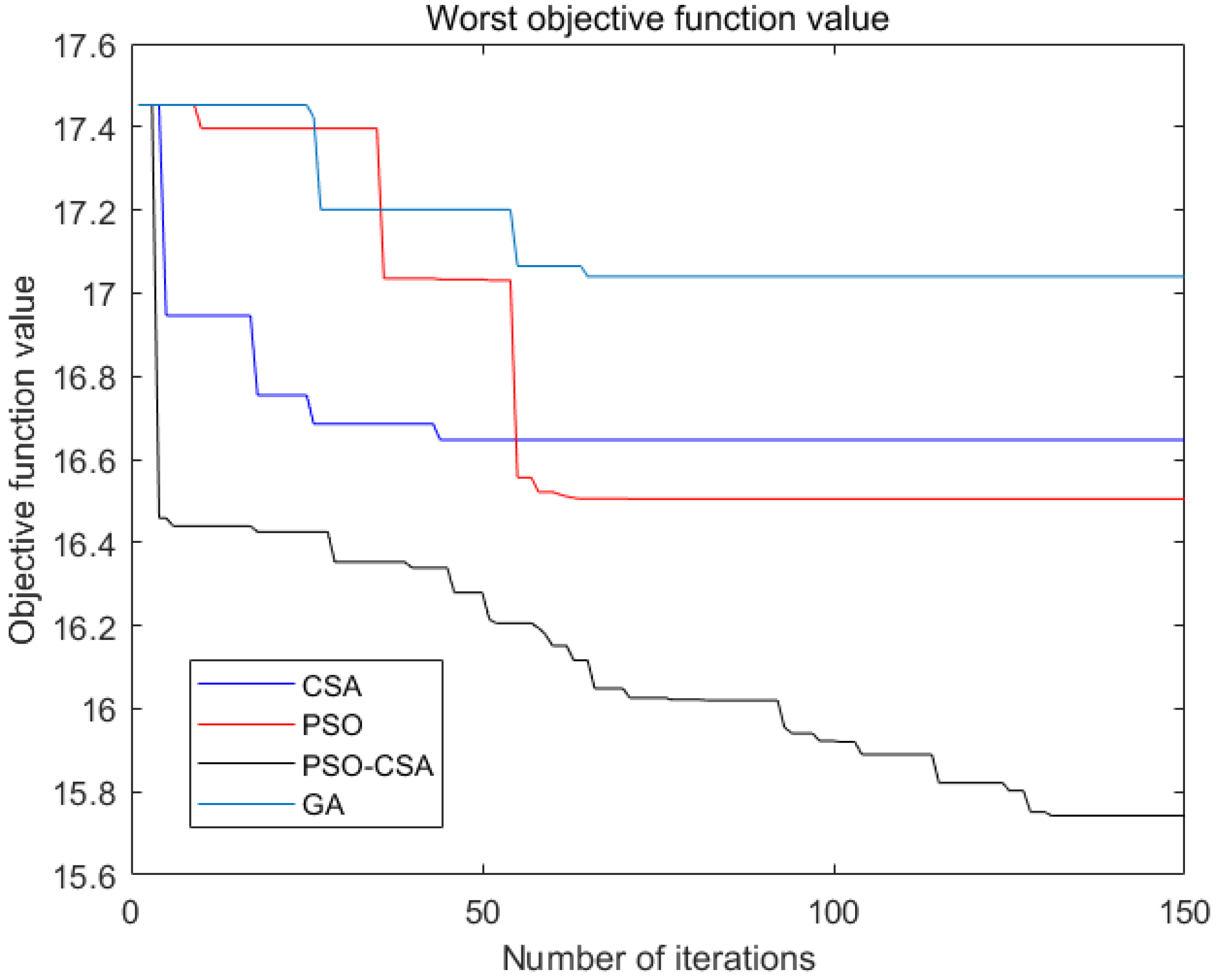
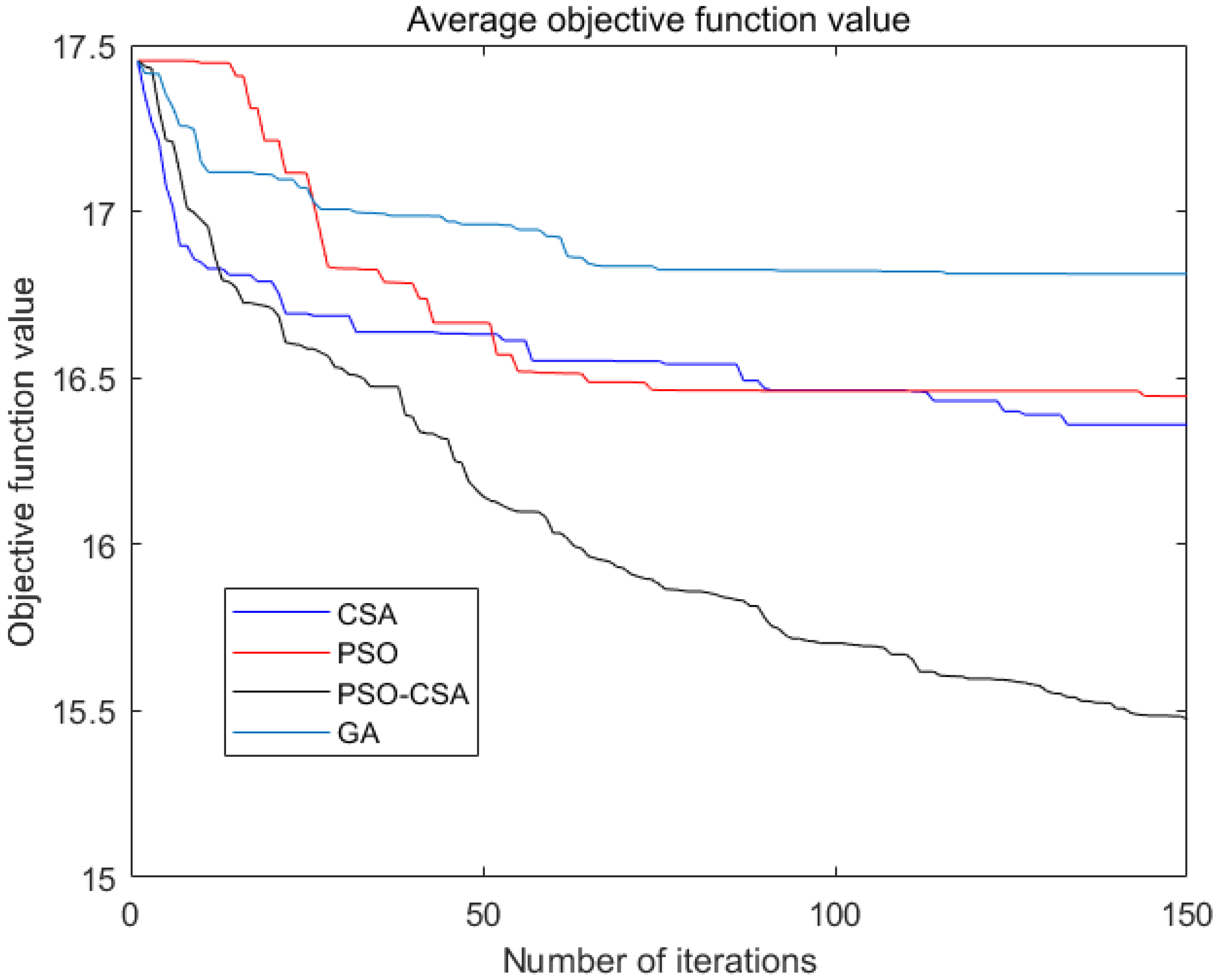
4.2. Display of Simulation Results

According to Figure 2 and Table 2, the industrial, agricultural, domestic and ecological water in the two water supply areas of water supply area I and II are provided by scheduling reservoir A and reservoir B. The CSA algorithm, the PSO algorithm, the GA algorithm and the PSO-CSA algorithm proposed in this paper are run 30 times, and the total convergence curve of the running process is shown in Figure 3, Figure 4 and Figure 5. Among them, Figure 3 shows the optimal convergence curves of the four algorithms during the 30 runs. Figure 4 shows the worst convergence curves of the four algorithms during the 30 runs of the four algorithms. Figure 5 shows the average convergence curve over the course of 30 runs of the four algorithms.

Further,

Table 3. The optimal value, the worst value and the average value of the fitness function of the four algorithms in the process of running 30 times.

Algorithm	CSA	PSO	GA	PSO-CSA
Index	Numerical Value
The optimal value	16.06	16.29	16.72	15.00
The worst value	16.55	16.50	17.04	15.74
The average value	16.36	16.45	16.81	15.48

shows the specific values of the optimal value, the worst value and the average value of the fitness function of the CSA algorithm, the PSO algorithm, the GA algorithm and the PSO-CSA algorithm during 30 runs.

In addition, the PSO-CSA algorithm proposed in this paper has been operated 30 times, and the water supply volume of reservoir A and reservoir B to the two water supply areas in each month (including the water supply volume provided by reservoir A/B to the industry, agriculture, domestic and ecology in water supply area I and II) are given under the optimal fitness function value, as shown in

Table 4. Outflow volumes of A and B reservoirs solved by PSO-CSA algorithm.

Month	1	2	3	4	5	6
Reservoir	$\mathbf{Water} \mathbf{Demand} (\mathbf{Unit}:\times {10}^4{\mathbf{m}}^3)$
A	1522.7	1613.4	3559.4	5216.5	6014.5	7534.7
B	1591.5	1733.2	2172.0	2208.1	2420.8	2505.0
Month	7	8	9	10	11	12
Reservoir	Water Demand (Unit:$\times {\mathbf{10}}^{\mathbf{4}}$m3)
A	7063.2	6110.1	2643.3	2621.8	1732.8	1769.7
B	2640.0	2791.45	2614.7	2386.9	1972.3	1723.1

.

4.3. Discussion

From Figure 3, Figure 4 and Figure 5, it can be seen that the results of the PSO-CSA algorithm are the best results, whether from the optimal convergence curve of the algorithm or from the worst convergence curve and average convergence curve of the algorithm. It can be seen from Table 3 that during the process of running the four algorithms 30 times, the optimal value of PSO-CSA algorithm is 15.00, 7.06–11.46% lower than that of the other three algorithms; the worst value of PSO-CSA algorithm is 15.74, 4.83–8.26% lower than that of the other three algorithms; the average value of PSO-CSA algorithm is 15.48, 5.68–8.59% lower than that of the other three algorithms. Therefore, it can be concluded that compared with the PSO algorithm, CSA algorithm and GA algorithm, the scheme presented in this paper has the best effect in the sustainable scheduling of reservoirs.

Within a scheduling period (one year), the water supplied by reservoir A to water supply area I is 47,402.1 $\times {10}^4$ m³, the demand of water supply area I is 49,724 $\times {10}^4$ m³, the average water supply guarantee rate is 95.33%, and the water deficit within one year is 2321.9 $\times {10}^4$ m³; reservoir B to water supply area II is 26,759.05 $\times {10}^4$ m³, the demand of water supply area I is 27,832 $\times {10}^4$ m³, the average water supply guarantee rate is 96.15%, and the water deficit within one year is 1072.95 $\times {10}^4$ m³. In addition, it is worth pointing out that the annual power generation of the PSO-CSA algorithm designed in this paper is 7.84–12.17% higher than that of the other three algorithms.

5. Conclusions

Considering the environmental demand for reservoir water resource dispatch, this paper establishes a multi-objective function from the benefit objectives, water supply objectives and environmental objectives of cascade reservoir scheduling. The real conditions such as the minimum ecological water limit, the maximum water level and the minimum water level limit of the reservoir were considered. In addition, in order to improve the convergence accuracy of the CSA algorithm, a PSO-CSA algorithm is designed to solve the problem. Experimental results show that the proposed algorithm has high superiority in solving the water resource scheduling of cascade reservoirs, and the annual power generation of the PSO-CSA algorithm designed in this paper is 7.84–12.17% higher than that of the other three algorithms. It should be pointed out that this paper does not consider the flood control objectives of cascade reservoirs, and in the process of further research, this paper will add flood control targets to the cascade reservoir scheduling model, so as to improve the model.

References

1. Ren, M.; Zhang, Q.; Yang, Y.; Wang, G.; Xu, W.; Zhao, L. Research and Application of Reservoir Flood Control Optimal Operation Based on Improved Genetic Algorithm. Water 2022, 14, 1272. [Google Scholar] [CrossRef]
2. Shang, L.; Li, X.; Shi, H.; Kong, F.; Wang, Y.; Shang, Y. Long-, Medium-, and Short-Term Nested Optimized-Scheduling Model for Cascade Hydropower Plants: Development and Practical Application. Water 2022, 14, 1586. [Google Scholar] [CrossRef]
3. Grigg, N.S. Large-scale water development in the United States: TVA and the California State Water Project. Int. J. Water Resour. Dev. 2021, 39, 70–88. [Google Scholar] [CrossRef]
4. Yao, H.; Dong, Z.; Li, D.; Ni, X.; Chen, T.; Chen, M.; Jia, W.; Huang, X. Long-term optimal reservoir operation with tuning on large-scale multi-objective optimization: Case study of cascade reservoirs in the Upper Yellow River Basin. J. Hydrol. Reg. Stud. 2022, 40, 101000. [Google Scholar] [CrossRef]
5. Dobson, B.; Wagener, T.; Pianosi, F. An argument-driven classification and comparison of reservoir operation optimization methods. Adv. Water Resour. 2019, 128, 74–86. [Google Scholar] [CrossRef]
6. Seibert, S.; Skublics, D.; Ehret, U. The potential of coordinated reservoir operation for flood mitigation in large basins—A case study on the Bavarian Danube using coupled hydrological–hydrodynamic models. J. Hydrol. 2014, 517, 1128–1144. [Google Scholar] [CrossRef]
7. Pan, Z.; Chen, L.; Teng, X. Research on joint flood control operation rule of parallel reservoir group based on aggregation–decomposition method. J. Hydrol. 2020, 590, 125479. [Google Scholar] [CrossRef]
8. Jiao, H.; Wei, H.; Yang, Q.; Li, M. Application Research of CFD-MOEA/D Optimization Algorithm in Large-Scale Reservoir Flood Control Scheduling. Processes 2022, 10, 2318. [Google Scholar] [CrossRef]
9. Ahmad, A.; Razali, S.F.M.; Mohamed, Z.S.; El-Shafie, A. The Application of Artificial Bee Colony and Gravitational Search Algorithm in Reservoir Optimization. Water Resour. Manag. 2016, 30, 2497–2516. [Google Scholar] [CrossRef]
10. Bashiri, H.; Qaderi, K.; Rheinheimer, D.; Sharifi, E. Application of Harmony Search Algorithm to Reservoir Operation Optimization. Water Resour. Manag. 2015, 29, 5729–5748. [Google Scholar] [CrossRef]
11. Fang, Y.; Ahmadianfar, I.; Samadi-Koucheksaraee, A.; Azarsa, R.; Scholz, M.; Yaseen, Z.M. An accelerated gradient-based optimization development for multi-reservoir hydropower systems optimization. Energy Rep. 2021, 7, 7854–7877. [Google Scholar] [CrossRef]
12. Bozorg-Haddad, O.; Janbaz, M.; Loáiciga, H.A. Application of the gravity search algorithm to multi-reservoir operation optimization. Adv. Water Resour. 2016, 98, 173–185. [Google Scholar] [CrossRef]
13. Bakanos, P.I.; Katsifarakis, K.L. Optimizing Current and Future Hydroelectric Energy Production and Water Uses of the Complex Multi-Reservoir System in the Aliakmon River, Greece. Energies 2020, 13, 6499. [Google Scholar] [CrossRef]
14. Ehteram, M.; Allawi, M.F.; Karami, H.; Mousavi, S.-F.; Emami, M.; El-Shafie, A.; Farzin, S. Optimization of Chain-Reservoirs’ Operation with a New Approach in Artificial Intelligence. Water Resour. Manag. 2017, 31, 2085–2104. [Google Scholar] [CrossRef]
15. Moravej, M.; Hosseini-Moghari, S.-M. Large Scale Reservoirs System Operation Optimization: The Interior Search Algorithm (ISA) Approach. Water Resour. Manag. 2016, 30, 3389–3407. [Google Scholar] [CrossRef]
16. Li, Y.-B.; Liu, Y.; Nie, W.-B.; Ma, X.-Y. Inverse Modeling of Soil Hydraulic Parameters Based on a Hybrid of Vector-Evaluated Genetic Algorithm and Particle Swarm Optimization. Water 2018, 10, 84. [Google Scholar] [CrossRef]
17. Recio Villa, I.; Martínez Rodríguez, J.B.; Molina, J.L.; Pino Tarragó, J.C. Multiobjective Optimization Modeling Approach for Multipurpose Single Reservoir Operation. Water 2018, 10, 427. [Google Scholar] [CrossRef]
18. Liu, H.; Sun, Y.; Cao, J.; Chen, S.; Pan, N.; Dai, Y.; Pan, D. Study on UAV Parallel Planning System for Transmission Line Project Acceptance Under the Background of Industry 5.0. IEEE Trans. Ind. Inform. 2022, 18, 5537–5546. [Google Scholar] [CrossRef]
19. Rashid, M.U.; Abid, I.; Latif, A. Optimization of hydropower and related benefits through Cascade Reservoirs for sustainable economic growth. Renew. Energy 2021, 185, 241–254. [Google Scholar] [CrossRef]
20. Babamiri, O.; Marofi, S. A multi-objective simulation–optimization approach for water resource planning of reservoir–river systems based on a coupled quantity–quality model. Environ. Earth Sci. 2021, 80, 389. [Google Scholar] [CrossRef]
21. Feng, Z.-K.; Liu, S.; Niu, W.-J.; Li, B.-J.; Wang, W.-C.; Luo, B.; Miao, S.-M. A modified sine cosine algorithm for accurate global optimization of numerical functions and multiple hydropower reservoirs operation. Knowledge-Based Syst. 2020, 208, 106461. [Google Scholar] [CrossRef]
22. Seifollahi-Aghmiuni, S.; Bozorg-Haddad, O. Simulation–Optimization Tool for Multiattribute Reservoir Systems. J. Hydrol. Eng. 2019, 24, 04019028. [Google Scholar] [CrossRef]
23. Feng, Z.-K.; Niu, W.-J.; Zhang, R.; Wang, S.; Cheng, C.-T. Operation rule derivation of hydropower reservoir by k-means clustering method and extreme learning machine based on particle swarm optimization. J. Hydrol. 2019, 576, 229–238. [Google Scholar] [CrossRef]
24. Chen, H.-T.; Wang, W.-C.; Chen, X.-N.; Qiu, L. Multi-objective reservoir operation using particle swarm optimization with adaptive random inertia weights. Water Sci. Eng. 2020, 13, 136–144. [Google Scholar] [CrossRef]
25. Ford, L.; de Queiroz, A.; DeCarolis, J.; Sankarasubramanian, A. Co-Optimization of Reservoir and Power Systems (COREGS) for seasonal planning and operation. Energy Rep. 2022, 8, 8061–8078. [Google Scholar] [CrossRef]
26. Sakthivel, V.; Thirumal, K.; Sathya, P. Short term scheduling of hydrothermal power systems with photovoltaic and pumped storage plants using quasi-oppositional turbulent water flow optimization. Renew. Energy 2022, 191, 459–492. [Google Scholar] [CrossRef]
27. Acuña, G.; Domínguez, R.; Arganis, M.L.; Fuentes, O. Optimal Schedule the Operation Policy of a Pumped Energy Storage Plant Case Study Zimapán, México. Electronics 2022, 11, 4139. [Google Scholar] [CrossRef]
28. Zhang, X.; Deng, L.; Wu, B.; Gao, S.; Xiao, Y. Low-Impact Optimal Operation of a Cascade Sluice-Reservoir System for Water-Society-Ecology Trade-Offs. Water Resour. Manag. 2022, 36, 6131–6148. [Google Scholar] [CrossRef]
29. Razavi, S.-M.; Momeni, H.-R.; Haghifam, M.-R.; Bolouki, S. Multi-Objective Optimization of Distribution Networks via Daily Reconfiguration. IEEE Trans. Power Deliv. 2021, 37, 775–785. [Google Scholar] [CrossRef]
Figure 1. Major cascade reservoirs of the California State Water Project (SWP).
Water 15 00578 g001
Figure 2. Topological structure diagram of cascade reservoir system in the Oroville–Thermalito Complex.
Water 15 00578 g002
Figure 3. Optimal convergence curves for the four algorithms.
Water 15 00578 g003
Figure 4. Worst convergence curves for the four algorithms.
Water 15 00578 g004
Figure 5. Average convergence curves for the four algorithms.
Water 15 00578 g005