Article

Hybridizing Artificial Intelligence Algorithms for Forecasting of Sediment Load with Multi-Objective Optimization

1
Department of CSE, Koneru Lakshmaiah Education Foundation, Vaddeswaram 522302, India
2
Department of Computer Science, Umm Al-Qura University, Mecca P.O. Box 715, Saudi Arabia
3
Department of Computer Science and Engineering, Chaitanya Bharathi Institute of Technology, Hyderabad 500075, India
4
Department of Project Management, Universidad Internacional Iberoamericana, Campeche 24560, Mexico
5
Higher Polytechnic School, Universidad Europea del Atlántico, 39011 Santander, Spain
6
Uttaranchal Institute of Technology, Uttaranchal University, Dehradun 248007, India
7
Faculty of Education, Curriculums and Teaching Department, Umm Al-Qura University, Makkah P.O. Box 734, Saudi Arabia
8
Department of CSE, Amrita Sai Institute of Science & Technology, Paritala 521180, India
9
Department of Project Management, Universidad Internacional Iberoamericana, Arecibo, PR 00613, USA
*
Author to whom correspondence should be addressed.
Water 2023, 15(3), 522; https://doi.org/10.3390/w15030522
Submission received: 25 November 2022 / Revised: 5 January 2023 / Accepted: 16 January 2023 / Published: 28 January 2023
(This article belongs to the Section Water Erosion and Sediment Transport)

Abstract

:
Forecasting of sediment load (SL) is essential for reservoir operations, design of water resource structures, risk management, water resource planning and for preventing natural disasters in the river basin systems. Direct measurement of SL is difficult, labour intensive, and expensive. The development of an accurate and reliable model for forecasting the SL is required. Sediment transport is highly non-linear and is influenced by a variety of factors. Forecasting of the SL using various conventional methods is not highly accurate because of the association of various complex phenomena. In this study, major key factors such as rock type (RT), relief (R), rainfall (RF), water discharge (WD), temperature (T), catchment area (CA), and SL are recognized in developing the one-step-ahead SL forecasting model in the Mahanadi River (MR), which is among India’s largest rivers. Artificial neural networks (ANN) in conjunction with multi-objective genetic algorithm (ANN-MOGA)-based forecasting models were developed for forecasting the SL in the MR. The ANN-MOGA model was employed to optimize the two competing objective functions (bias and error variance) with simultaneous optimization of all associated ANN parameters. The performances of the proposed novel model were finally compared to other existing methods to verify the forecasting capability of the model. The ANN-MOGA model improved the performance by 12.81% and 10.19% compared to traditional AR and MAR regression models, respectively. The results suggested that hybrid ANN-MOGA models outperform traditional autoregressive and multivariate autoregressive forecasting models. Overall, hybrid ANN-MOGA intelligent techniques are recommended for the forecasting of SL in rivers because of their relatively better performance as compared to other existing models and simplicity of application.

1. Introduction

Hydrology deals with the efficient utilization of water resources and their management through the use of hydrological forecasting. Forecasting sediment load (SL) is an important concern in water resource management, and it is essential to know information about reservoir operations, water resource planning, flooding, water pollution control, reservoir design in rivers, and risk management as well as for preventing natural disasters [1,2]. Moreover, SL forecasts are required for decision making and policy formulation in a variety of sectors such as hydropower, flood control, reservoir sedimentation, and reservoir operations [3]. Knowledge of the amount of SL in a river at a particular time can lead to better knowledge of flood potential and consequently help control over-bane flooding. The amount of accumulated sediment in a reservoir is a crucial factor in determining the reservoir’s service life [4]. As a result, it is becoming increasingly important to measure SL, but it is challenging due to the complexity and non-linearity of the interactions of the various controlling factors with SL.
Jansson [5] demonstrated the effect of river basin features such as geology, storage capacity, soil, and relief (R) on SL. Syvitski et al. [6] revealed that long-term sediment discharge is associated with basin area and basin R, which was employed to examine the effects of climate change globally on the flux of sediment of the world’s rivers. The SL in the river is caused by the physical as well as chemical weathering of the soil and rock within the basin. The catchment area (CA) affects SL due to variations in the properties of the catchment such as the capacity of storage and gradient [7]. In most of the world’s major rivers, a good non-linear association between SL and water discharge (WD) has been found [8,9]. River sediment transportation and generation are significantly influenced by climatic variables such as temperature (T) and rainfall (RF) [10]. To design the numerous SL forecasting models based on prior research, temporal data such as WD, RF, SL, and T, as well as spatial data such as rock type (RT), R, and CA were taken into consideration.
The data-driven and physically based models are used for forecasting water resources [11]. The physically based models require a lot of data and use complicated mathematical equations to incorporate the physical process. Traditional time series regression models such as Autoregressive (AR), Autoregressive Moving Averages (ARMA), and Autoregressive Integrated Moving Averages (ARIMA) have been extensively used for hydrological time series forecasting [12]. These models have a lot of required input parameters, and most traditional modeling techniques suppose the data are linear and stationary, which makes them incapable of handling non-stationary and non-linearity processes associated with hydrology [13]. There are various non-linear forecasting methods that are also used for forecasting SL but those are also not capable of forecasting the SL accurately and efficiently [13]. Artificial intelligence (AI) data-driven methods have shown promise in modeling and forecasting non-stationary and non-linear processes in water resources, as well as in dealing with huge amounts of dynamicity and noise hidden in datasets. The drawbacks of linear AR, ARMA, and ARIMA and non-linear autoregressive networks with exogenous inputs forecasting models of SL can be overcome by using an AI-based non-linear system [13,14]. Long- and short-term forecasts are critical in reservoir operational processes, which are typically planned every month. Many researchers developed AI-based SL forecasting models using various controlling factors based on monthly data [15,16,17].
The goal of this research is not to describe the superiority of one technique over others, but rather to demonstrate that different modeling parameters must be chosen judiciously to generate a generalized, accurate, and reliable model. The ANN is chosen as a non-linear approach amongst AI techniques because it is currently among the most popular known AI techniques. The ANN works on the principle of the biological brain and the nervous system that goes along with it. Through proper learning, the ANN is capable of identifying the complex non-linear or linear relationship between outputs and inputs data without detailed knowledge of the character of the internal structure of physical processes. The ANN can establish non-linear links among outputs and inputs and makes them flexible and useful techniques for modeling the phenomena of hydrology [18]. It is useful for modeling when the physical presence of a process is unsure, there is no mathematical form for a description of the process, and reasonable experimental data are available [18,19]. The ANN is widely used in hydrology for forecasting the RF, runoff, flood, river discharge, and sediment yield modeling, which provide better results than the traditional regression-based forecasting models [14,20,21,22]. Nevertheless, the ANN models possess some drawbacks such as overfitting and underfitting and local minima problems due to inaccurately choosing the ANN model’s parameters (hidden node size, network topologies, number of hidden layers, nodes in hidden layers, initial weights, etc.) using greed search or trial-and-error approaches [23,24]. These ANN parameter selection approaches require a huge amount of computing time to calculate the parameter value and do not guarantee to provide an optimum solution [24]. It is possible to implement the genetic algorithm (GA) to solve the issues with ANN. The GA algorithm is a population-based global optimization algorithm that is based on Darwin’s theory of evolution and is used to find the best parameters for ANN models. It generates diversity in a population of individuals (chromosomes) by employing various genetic operators such as mutation, selection, and crossover, and then provides the best solutions. Nowadays, the GA is among the most popular algorithms for global search optimization which is hybridized with ANN to overcome ANN’s drawbacks [24,25]. The concurrent optimization of related parameters in ANN models using GA has been used to overcome the shortcomings of trial-and-error procedures as shown by a variety of applications of AI models. Numerous studies demonstrate that this strategy not only reduces the amount of computation required but also yields better results [26,27,28].
The ANN model parameters are optimized using GA by optimizing a single objective, namely Mean Square Error (MSE), as a criterion for the evaluation of performance, which is found in various studies [29,30]. Furthermore, the performance of feed-forward back-propagation ANN is also determined by achieving the lowest possible MSE [31]. The drawbacks of using a single objective (MSE) for the optimization of parameters of ANN have been well documented in past research [31,32]. The MSE is a summation of error variance and squared mean error (bias). MSE minimization does not guarantee that both error variance and bias are minimized. There is a conflict between bias (mean error) and variance, both of which affect ANN performance (MSE) [32]. In influencing MSE of estimation or forecasting, bias and variance contradict each other, resulting in significant uncertainty in evaluation. If one of them is reduced, then the other is increased [33]. Thus, the model selection issue can be viewed as a multi-objective optimization issue. As a result, minimizing both components is critical for attending generalization to avoid overfitting or underfitting with greater accuracy. Underfitting is caused by bias, whereas overfitting is caused by variance, which limits the model’s generalization ability and contributes to its poor performance [31]. The optimization and compromise of bias and variance multi-objectives result in a reliable and accurate model [34,35]. The GA is a well-suited population-based search method for problems involving multiple objectives [19,36]. The Non-Dominated Sorting GA (NSGA), Controlled Elitist GA (CEGA), and Elitist Non-Dominated Sorting GA (NSGA-II) are more familiar with GA-based multi-objective algorithms [37]. Controlled Elitist Gas are more capable of maintaining population diversity for getting to the best Pareto front by controlling the number of elites than NSGA-II and NSGA [35]. Therefore, the Controlled Elitist MOGA-based ANN model has been used to optimize these two contradicting responses (variance and bias). Recently, many works of literature are available in various fields for prediction and forecasting using multi-objective optimization for ANN and it was found that the system’s accuracy could be increased using this hybrid approach [38,39,40]. Rosales-Pérez [33] applied multi-objective GA for the optimization of AI models such as Support Vector Machine (SVM) parameters by optimizing bias and variance. Recently, there are few studies that have been conducted on the multi-objective optimization-based model to estimate the sediment load or suspended sediment concentration [41,42].
In this study, forecasting is a term that is used when inputs are past monthly time series of temporal data such as Q, RF, and T, as well as spatial data such as RT, R, and CA, and output data are the SL. Thus, this paper deals with the forecasting of the SL using the past observed SL data and other observed variables (RF, WD, and T) with spatial data (RT, CA, and R). This study was conducted in the MR system. Various researchers have used monthly one-step-ahead forecasting studies in hydrology [43,44,45]. In this study, multi-objective genetic-based ANN forecasting models are developed for one-step-ahead of forecasting the SL in the MR basin with optimization of all ANN parameters (hidden layer neurons, combination coefficient, transfer function, inputs, bias weights, and connection weights) simultaneously.
Flood forecasting in the MR is studied by Kant et al. [46] with the use of a multi-objective evolutionary Neural Network (NN) and bootstrap NN. As per the author’s knowledge, no researcher has yet attempted to develop a fully automatic, highly generalized, globally single hybrid AI-based forecasting model. In this study, a fully automated parameter tuning and highly generalized AI forecasting model is developed for forecasting of SL in the Mahanadi River, which reduced the need for human intervention. The proposed model would replace the use of multiple models to predict the SL, which stands for suspended sediment load. This single model was applied at each gauging station to forecast the SL in the MR Basin. In this study, a single hybrid ANN-MOGA model was developed for effectively forecasting the SL at individual stations in the MR using a huge number of combinations of temporal (SL, T, RF, and WD) and spatial (RT, CA and R) data of 11 gauge stations. All parameters for the ANN model were optimized concurrently using the multi-objective GA, which included bias and variance objectives. These approaches d not only improve the model’s performance, but also significantly reduce computational time by eliminating grid searches and trial-and-error exercises. The forecasting capability of hybrid models was tested by comparing their performances to traditional Multivariate Autoregressive (MAR) and Autoregressive (AR) methods. It was revealed that the best accuracy was provided by the multi-objective GA-based ANN model with more generalization and it is the most suitable substituent among other comparative methods for forecasting the SL. If SL measurement is not possible, then approaches for multi-objective GA-based ANN modeling can be recommended for forecasting SL due to their ease of implementation and relatively better performance than other existing methods.

2. Study Area

To make the SL forecast, the MR basin was chosen. Flowing to the east, this river is a major waterway in the Indian peninsula (Figure 1). It is the fourth largest river in India and drains an area of 141,589 km2 or approximately 4.3% of India’s total land area [46]. Odisha receives 53% of the river’s basin area, while Chhattisgarh receives 46% and Maharashtra, Madhya Pradesh, and Jharkhand share the remaining 1% [46]. Until it enters the Bay of Bengal, the river flows for a total of 851 km. Thr MR was located between 19°20′ and 23°35′ north, and 80°30′ and 86°50′ east. The MR contains the Hirakud dam which is the world’s largest earthen dam. In terms of current sediment load, the MR is second among Indian peninsular rivers. Figure 1 shows the MR basin elevation map and the locations of all 11 hydro-climatological sites. The average annual RF was between 1200 and 1400 mm [47]. Approximately 90% of the yearly RF that the MR basin receives occurs during the monsoons. The MR basin has a dispersed pattern of RF strength. In the MR basin, the warmest months are April and May, with summer temperatures of 39 to 45 °C, and the coldest months are December and January, with winter temperatures of 4 to 12 °C [47]. The two largest bodies of water in the MR are Lake Chilka and the Hirakud Dam.

3. Methodology and Data

The preliminary processing includes data normalization that was proposed before developing the models. To maintain uniqueness while developing a model, data normalization is used to remove the ranges between the datasets. It revealed convergence and fast processing throughout training and minimized forecasting errors [49].
Data standardization is another name for the process of normalizing numerical data, which results in much more highly accurate network training. The range of all variables is fixed at 0 to 1 by the normalization process which is described briefly in different literature [24,48].
Data normalization’s primary goal is to remove the various ranges and dimensions of the variables included in the dataset. The normalization process of the data in the range of a   and b is performed using Equation (1):
C n o r m = a + C i C m i n C m a x C m i n × ( b a )
where C i is the ith actual value, C n o r m is the normalized value of C i , C m a x is the highest value, and C m i n is the lowest value of the dataset. In this case, “a” represents the lowest value, and “b” represents the highest value of normalized data.
The used data consist of monthly RF, T, WD, and SL during the years 1990–2010 and spatial variables such as R, CA, and RT of eleven gauging stations in the MR for developing the proposed models. Figure 1 depicts the locations of all these stations. The dataset from the individual station is partitioned: training data (70%) are used to develop the models; validation data (15%) are used to avoid model overfitting, while testing data (15%) are used to evaluate the model’s performance in a testing phase. Data from tests are regarded as “unseen” and “not used” in the process of modeling. Single testing, training, and validation for the MR basin were eventually produced by combining the data from all 11 stations. In this study, the forecasting of SL is performed using an ANN with a Multi-Layer perceptron (MLP) feed-forward using a Levenberg–Marquardt (LM) backpropagation algorithm. A wide variety of weight optimization strategies can be utilized during the training process of the MLP-based ANN; however, the LM training algorithm trains more quickly than the gradient descent training algorithm and achieves convergence more quickly [50]. The weight updating rule of ANN is presented as [24,50]:
W k + 1 = W k ( J T J ) + µ I ) 1 J T e
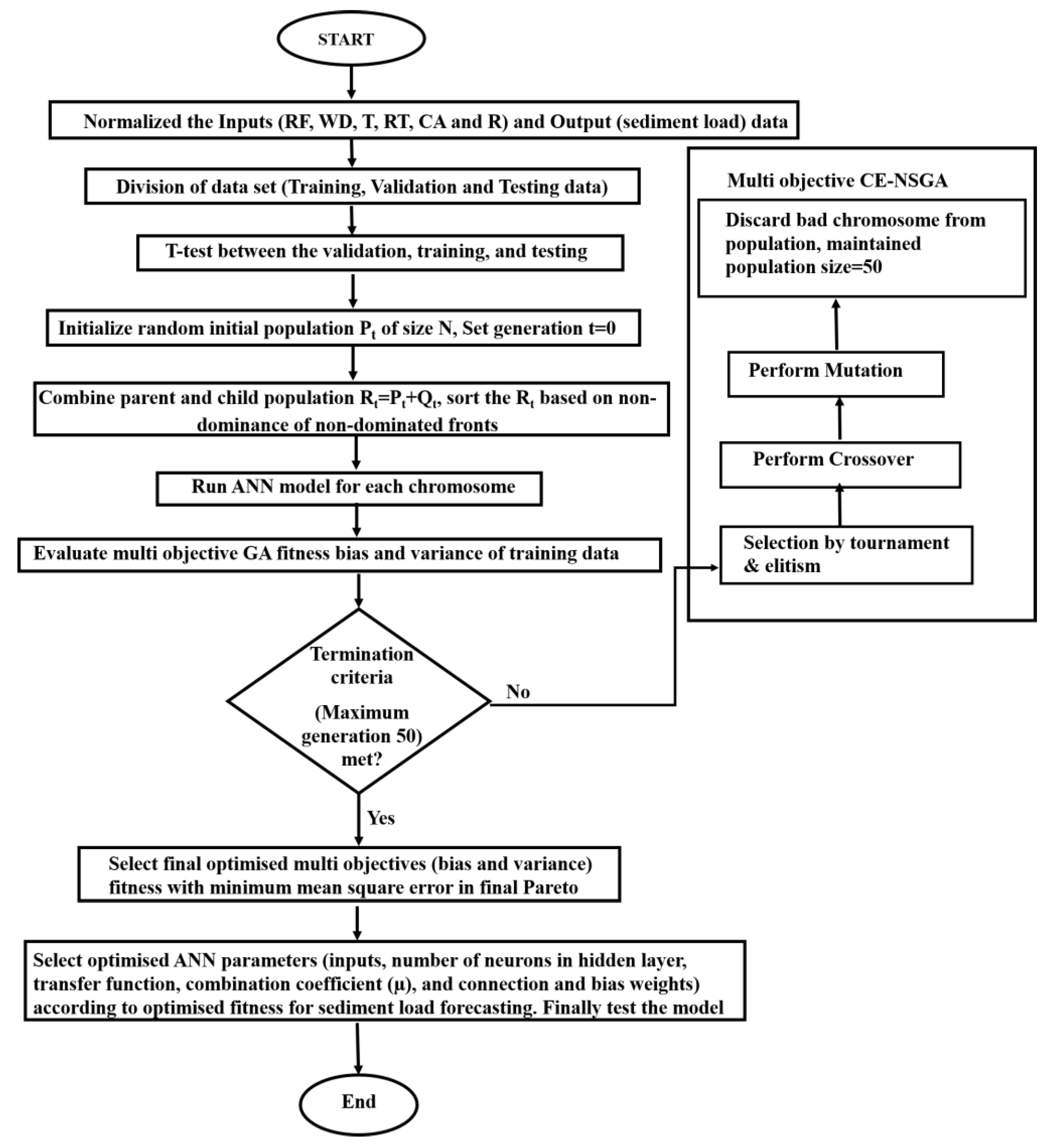
in which J is a Jacobian matrix, e is an error matrix, I represents an identity matrix, W is the weight of the ANN, and µ represents the combinational coefficient of LM, which plays an important role in the learning process of LM in an ANN. The flow chart of the ANN-MOGA method that has been proposed is shown in Figure 2.
Numerous artificial intelligence models have been successfully applied by various researchers for the prediction and forecasting in water resources [51,52,53,54,55]. The details description of MLP and LM training algorithms of ANN are discussed by various researchers [48,56]. Numerous factors affect the effectiveness of MLP-based ANN models, including the transfer function and number of nodes in the hidden layer, and the initial weights. If any of these factors is chosen incorrectly, the ANN will be poor, and the likelihood of the solution reaching the global optimum will be low. The GA has proven to be effective in resolving the issues of the ANN [27,57]. So, this research demonstrates the use of GA in ANN to overcome the drawbacks of ANN for forecasting SL with a selection of all ANN model parameters optimally. In this study, the output demonstrates the value at time frame t in the time series models of SL forecasting if the forecasting model’s inputs cover values corresponding to points of time t 1, t 2, t 3,..., t     n . In this study, the GA is used to choose the transfer function, inputs, neurons, combinational coefficient of LM ( µ ), bias, and connection weights. These are the five most important ANN parameters for SL forecasting. These ANN model parameters can be found in the chromosome, which is a binary string. The input parameters are found in the first part of the chromosome.
In the second part of the chromosome, a 3-bit binary number shows the transfer function for the hidden and output layers. In this section, the transfer functions in the output layer and the hidden layer are shown. Transfer functions are available in three different types: linear, log sigmoidal and tan sigmoidal. There are nine different ways to use transfer functions for the hidden and output layers. In the third part of the chromosome, 5 bits stand for the neurons in the hidden layer. During modeling, this binary number is turned into a decimal number. This is performed to make the hidden layer neurons. Due to the complexity and cost of processing the model, hidden neurons are limited to 32. All of the decimal numbers from 1 to 32 can be shown with 5-bit chromosomes. The 4th part of the chromosome denotes the µ, which is an 8-bit binary number. The µ showed decimal values from 0 to 255, which is normalized between 0.0010 and 9×10⁹ [24]. In the fifth section, the biases and weights of the connections of ANN models are shown. The length of the chromosome changes because the number of hidden neurons and the number of inputs change. The ANN-MOGA forecasting models are designed with GA parameters such as the number of generations, the size of the population, the rate of mutation, and the probability of a crossover. In this study, a uniform crossover with a high probability value (0.6) and a low probability of constant mutation (0.05) was used. The values of each chromosome’s fitness are estimated using the fitness function (RMSE) of the training dataset. The maximum generations (50) were considered as stopping criteria.
Both objective functions assessed the fitness values of each chromosome for the initial population. The chromosomes were sorted using a controlled non-dominating sorting strategy. In non-dominating sorting, the population was arranged according to the non-dominance level on various fronts (referred to as levels) [36]. To determine whether the solution does not predominate in the population, the following guidelines are used:
Bias [i] > Bias [j] and Variance [i] ≥ Variance [j]
or
Bias   [ i ]     Bias   [ j ]   and   Variance   [ i ]   > Variance   [ j ] ,   i j
where the chromosome numbers i and j are used. The solutions of the same non-dominated front are compared to establish the solution’s overall ranking after the non-dominated fronts are obtained. To compare solutions from the same non-dominated front, a crowding distance is used [36]. The final step was to obtain the solutions’ overall rank using the crowded-comparison operator, which combines the crowding distance and the measure of non-dominated rank. The multi-objective GA framework iteratively improves the beginning chromosomes according to their overall rank through various genetic operational processes, such as mutation, crossover, and selection. The tournament selection approach was used to make the decision [58]. The chosen chromosomes were subjected to crossover and mutation operations. Every generation also known as an iteration was followed by the crossover operation, which involved swapping out a portion of the binary strings of the available solutions to produce better individual solutions. According to the user selected mutation rate, the mutation operation is carried out by randomly flipping bits (0–1 or 1–0) of the chromosomes in order to diversify the existing solutions and avoid trapping at local minima. A child population Q0 of size N is produced by the mutation, selection, and crossover operators at iteration 0. The overall number of chromosomal solutions for any iteration t following the genetic operations is Rt = Pt ∪ Qt becomes twice (2N). P and Q represent the parent and child populations, respectively. R represents the total number of chromosomal solutions after the genetic operations. The objective functions of each solution (Rt) were determined by calculating, and the solutions have been ranked using the previously discussed Non-Dominated Sorting criteria and crowding distance. The rest solutions were eliminated from the solution space, and the top N solutions determined by their whole rank were chosen (referred to as elitism) for the following generation. The maximum number of individuals permitted from the ith non-dominated front as shown in Equation (5) is provided diversity in the new population, based on the geometric distribution [36].
N × ( 1 r 1 r K ) × r i 1
where K indicates the number of undominated fronts and r represents the reduction rate, which has a value lower than 1.
The proposed study combined the Controlled Elitist NSGA (CE-NSGA) and ANN models. The CE-NSGA is a more familiar GA-based multi-objective algorithm. The CE-NSGA has more capability to maintain the diversity of population for convergence to an optimal Pareto front by controlling elite numbers. The ANN model was used to find the two objectives such as error variance and mean error in CE-NSGA for ranking of non-dominated. The ideal parameters for the ANN model were chosen based on the most optimal solution from the final CE-NSGA generation. With these best ANN parameters, the ANN model can be applied to forecast the river system’s SL with given known input parameters. Figure 2 shows the flow chart for the multi-objective GA-based ANN model. In this study, AR forecasting models are designed by the linear combination of previous data of the variable (SL). The AR model is a fundamental class of time series model.
The AR model’s equation is presented below [12]:
SL t + 1 = a 0 SL t + a 1 SL t 1 + a 2 SL t 2 + + a n SL t n      
where n is the number of orders for the AR model, and ai ( i = 0, 1, 2,....., n ) represents the regression model’s coefficients. The MAR was designed using training datasets and the linear combination of the Autoregressive of multiple variables (WD, T, RF, and SL and spatial variables (R, CA, and RT). The MAR formula is shown below
SL t + 1 = a 1 WD t + b 1 RF t + c 1 T t + d 1 SL t , + a 2 WD t 1 + b 2 RF t 1 + c 2 T t 1 + d 2 SL t 1 + + a n WD t n + b n RF t n + c n T t n + d n SL t n   + e RT + f R + g CA
The linear MAR forecasting model is represented by this equation up to n lags. The ai, bi, ci, di, e, f, and g (i = 1,2, 3,…, n) represent the coefficients of the MAR model. The ai, bi, ci, and di represent the coefficients of WD, RF, T and SL, respectively. The coefficients of the RT, R, and CA are represented by the values e, f, and g, respectively. The maximum lag (n) in AR and MAR model for the SL forecasting is 12, after which the cyclicity begins due to seasonal behaviour of the data. There are four temporal variables: WD, SL, RF, and T. The RT, CA and R are the spatial variables.

4. Results and Discussion

4.1. Data Analysis

The non-linear comparison between different parameters is found using Spearman rank correlation coefficients which are presented in Table 1. The Spearman rank correlation of T and SL, RF and SL, and WD and SL are represented by r3, r2, and r1, respectively. The WD and SL have a significant and high Spearman rank correlation coefficient value which is represented by r1. It is found that SL has comparatively smallest and greatest values of the Spearman rank correlation with the WD at the Kntanmal and Rajim, respectively among all gauging stations (Table 1). The Pearson rank correlation coefficient between RF and SL has a significant value (greater than 0.5 at all eleven gauging stations) which is represented by r2. It shows that RF is significantly correlated with the SL.
Furthermore, it is observed from Table 1 that the Spearman rank correlation coefficient between T and SL is small and insignificant which is represented by r3. This indicates that T has an indirect effect on SL and did not directly contribute significantly to SL. It is found that the SL data have the greatest coefficient of variation value, maximum/mean, skewness, and Kurtosis among all hydro-climatic data (WD, RF, T, and SL) in the MR which indicates that the SL is more dispersed than the other parameters (WD, RF, and T), as well as extremely erratic and complicated, with a non-normal distribution in the MR basin [24]. Thus, forecasting SL by the model is very difficult as compared to the other variables.
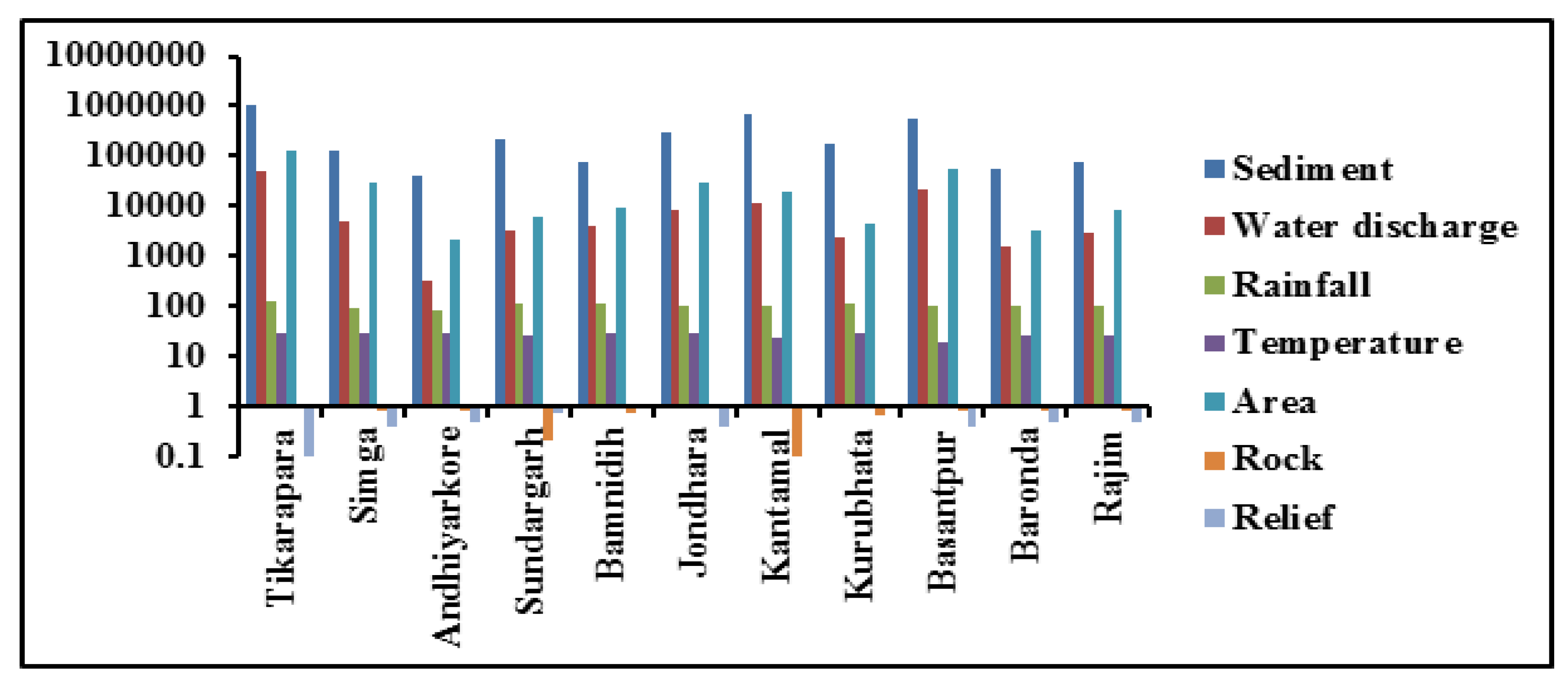
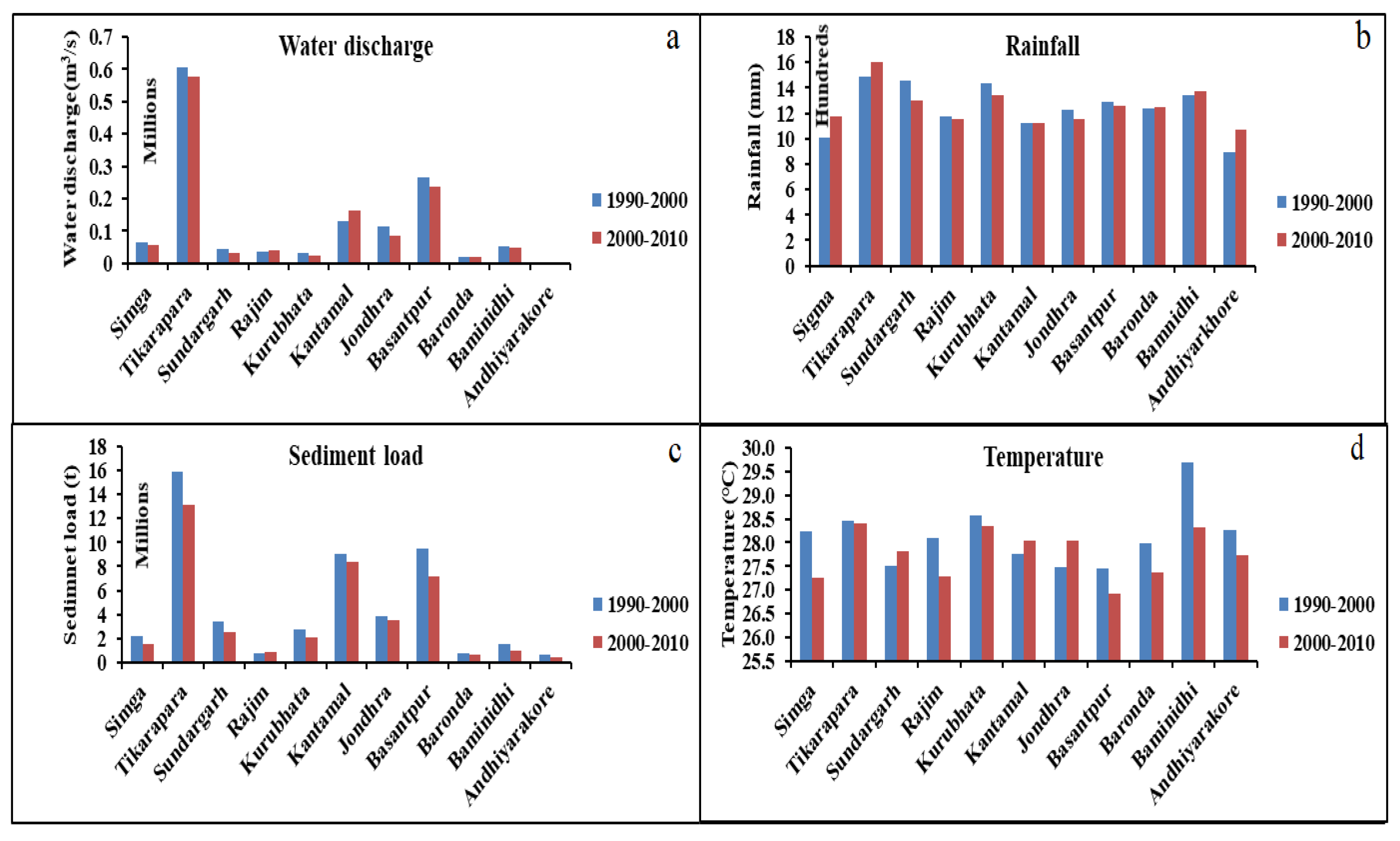
There were significant temporal as well as spatial variations in the SL. Variations of monthly average WD, RF, T, and SL data over 20 years with spatial variation (R, RT, and CA) of each gauge station in the logarithm scale are shown in Figure 3. Due to huge variations in the dataset, we have followed the logarithm scale so that maximum data values are shown in Figure 3. It is seen in Figure 3 that the pattern of decrease in WDs and corresponding sediment load is the same sediment load, except for Kantamal station. Further, Tikarapara station indicates the highest WD, CA, R, RF, and SL, whereas Andhiyarakore station shows the lowest values of it. Furthermore, it has been noted that SL changes proportionally with WD, with the Tikarapara gauge station recording the highest values due to the highest WD amongst all gauge stations. The highest CA is also observed at this gauge station. Lowest R is found at the Bamnidih. The lowest rock value is found at Kantamal. Variations in RF, WD, T, and SL during the decades of 1990–2000 and 2000–2010 at different locations such as upstream, midstream, and downstream in the MR are given in Figure 4. The highest decrement in sediment yield is found at Tikarapara station among all stations. This may have been caused by the SL trap at the Hirakud dam, which is upstream of the Tikarapara. Higher amount of SL is also decreased at Basantpur gauging, which may be due to traping of SL at large Minimata Bango dam nearest to this station.
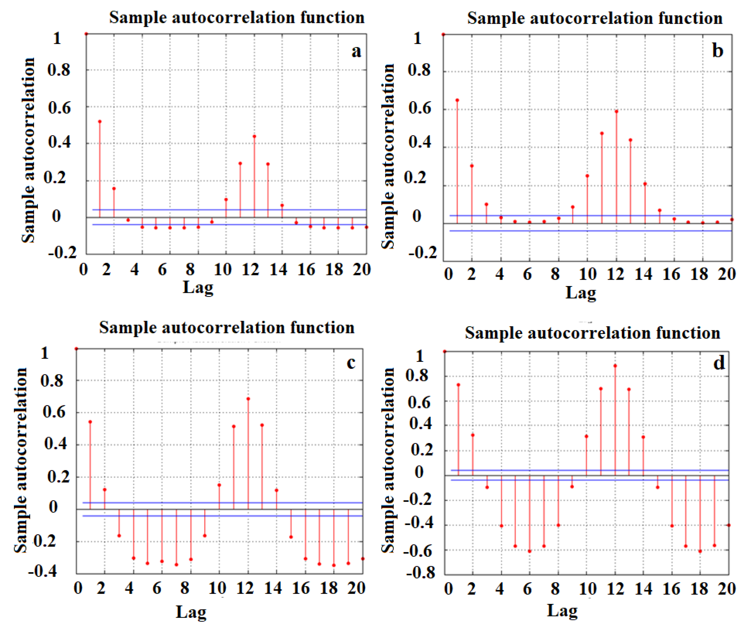
Since the SL, WD, RF, and T data are seasonal and available monthly, they are influenced by the data from the previous month. The maximum lag for the forecasting model must be selected. To evaluate the temporal correlations of SL, WD, RF, and T, an Autocorrelation Function (ACF) is employed. Figure 5 depicts the ACF of the SL with different time lags. The highest correlation was found at lag 1, and it decreases as the time lag increases (Figure 5). Additionally, it was noticed that ACF exhibited the next highest peak value at lag 12, supporting the seasonality of the SL dataset. The ACF plot illustrates that the highest lag is 12, after which seasonal data behavior indiciate cyclicity.

4.2. ANN-MOGA Forecasting Model

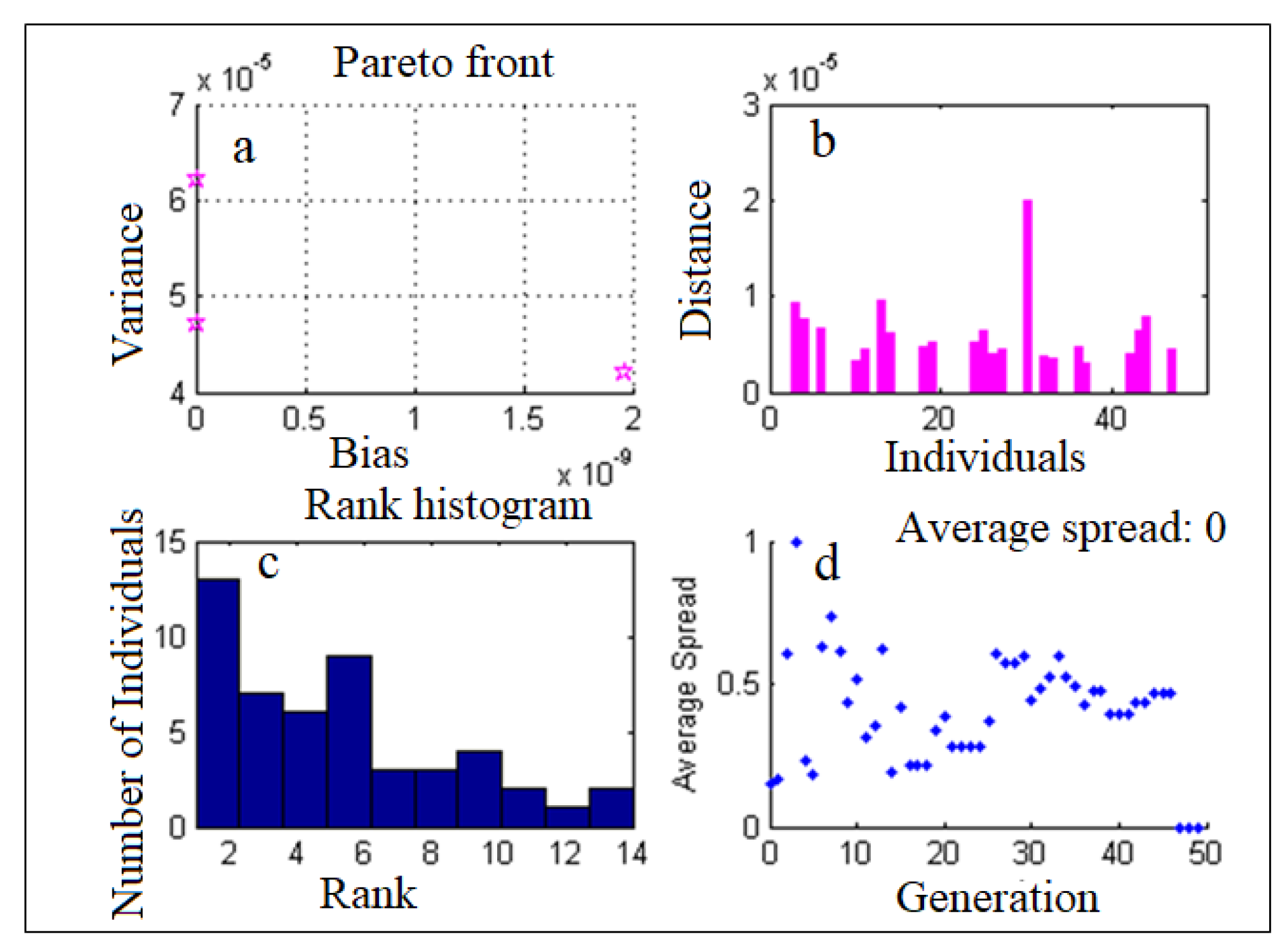
A set of final solutions in the form of Pareto solutions have been provided by the model at predetermined stopping criteria that correspond to the highest number of generations (50). Figure 6a depicts the variation in bias and variance during the training stage. In the training stage, MSE (0.00352) and its subsequent variance value (0.000651) and bias (0.00424) were found to be the best Pareto solution. Figure 6b shows the variation in crowding distance among individuals. Figure 6c displays the rankings of the individual. Figure 6d illustrates the Pareto average spread variation with generation.
Table 2 lists the various types of models with lag input variables. The ANN-MOGA-51 models are built using previous time series of temporal variables (WD, R, SL, and T) with 12 lags for each variable and 3 spatial variables (CA, RT, and R). The ANN-MOGA-48 models are built on prior time series temporal data (WD, R, SL, and T) with 12 lag for each variable and without considering the spatial data. The ANN-MOGA-15 model is developed by 15 input variables (12 lag time series inputs of SL and 3 spatial factors) for forecasting one-step-ahead of SL.
The ANN-MOGA-12 models are established using previous time series SL only data with 12 lags. The lag for each temporal data (RF, T, WD, and SL) is twelve. All of these models’ performances are compared to assess the forecasting capability of models as per statistical error analysis. The statistical error is used as an evaluation metric, and the performances of the different models are compared to one another to determine which model performs the best. Validation, training, and testing dataset are assessed to evaluate error statistics such as the Mean Square Error (MSE), the correlation coefficient (r), the Root Mean Square Error (RMSE), the Mean Absolute Error (MAE), and the error variance (VAR) for the forecasting models.
RMSE = ( i = 1 N ( O i F i ) N ) 2
MSE = ( i = 1 N ( O i F i ) N ) 2
MAE = i = 1 N | O i F i | N
r = i = 1 N ( O i O ¯ i ) ( F F ¯ i ) i = 1 N ( O i O ¯ i ) i = 1 N ( F i F ¯ i )
VAR = i = 1 N ( E E ¯ ) 2 N
where, O i , O i ¯ , F i and F i ¯ are measured, measured mean, forecasted and forecasted mean values, respectively. The N value represents the number of samples. The E ¯ and E represent the mean error and error values.
All hybrid multi-objective GA-based ANN hybrid forecasting models use statistical errors obtained from testing, validation, and training datasets for one-step-ahead forecasting of the SL value, which is presented in Table 3. The statistics of all errors of testing, validation, and training data for the ANN-MOGA-12, ANN-MOGA-48, ANN-MOGA-15, and ANN-MOGA-51 models reveal that r is relatively high, while error variance, RMSE, MAE, and MSE are all low. It can be implied that these models are highly accurate at predicting SL. High levels of consistency across the three datasets show that generalized forecasting models were produced and that neither overfitting nor underfitting occurred. Among all comparative models, the ANN-MOGA-51 model stands out as the best. Table 4 lists the GA-optimized parameters chosen for the designed ANN-MOGA models. Two and twenty-nine are the optimum combinational coefficient (µ) and neurons, respectively. Pure linear and log sigmoidal transfer functions are optimally selected at the output layer and hidden layer, respectively, in the ANN-MOGA-51 model. Twenty-nine neurons are the best number for an ANN model’s hidden layer. After the evolution run, the best-fit chromosomes were used to determine the best solution for the ANN- MOGA-51 model.
Table 5 displays the error statistics for the 11 gauge stations determined with the best ANN-MOGA-51 model. It is also clear from Table 5 that there is a wide range of performance between the stations, with some stations providing good performance and others showing poor performance. The unpredictable and complex non-linear nature of SL delivers the forecasting model incapable of providing accurate forecasts of SL at the Andhiyarakhore and Baronda stations. The forecasting model’s inaccuracy is a direct result of the low CA and the flat land. Located in the Raipur district of Chhattisgarh, India, Simga is the first gauging station of the MR after its origin near Nagri town and Pharsiya village. Both WD and SL are low at this station. At the Simga station, the forecasting model is providing worse results. Due to the high coefficient of variation (COV), max/mean ratio, skewness, and kurtosis value of influential parameters, many AI models were not performing well at some MR stations [36]. Forecasted and actual SL have a high degree of correlation at the Tikarapara, Kurubhata, and Jondhra gauging stations (r values greater than 0.7). This reveals the proposed model’s high performance at these locations. The r value of 0.4780 for the Basantpur gauge station is not significant. Poor correlation between the WD and SL, caused by the large Minimata Bango dam upstream of this station, contributes to the proposed model’s bad performance at this location. The remaining gauging stations have a significant r value between 0.5 and 0.7, indicating a moderate correlation [59].
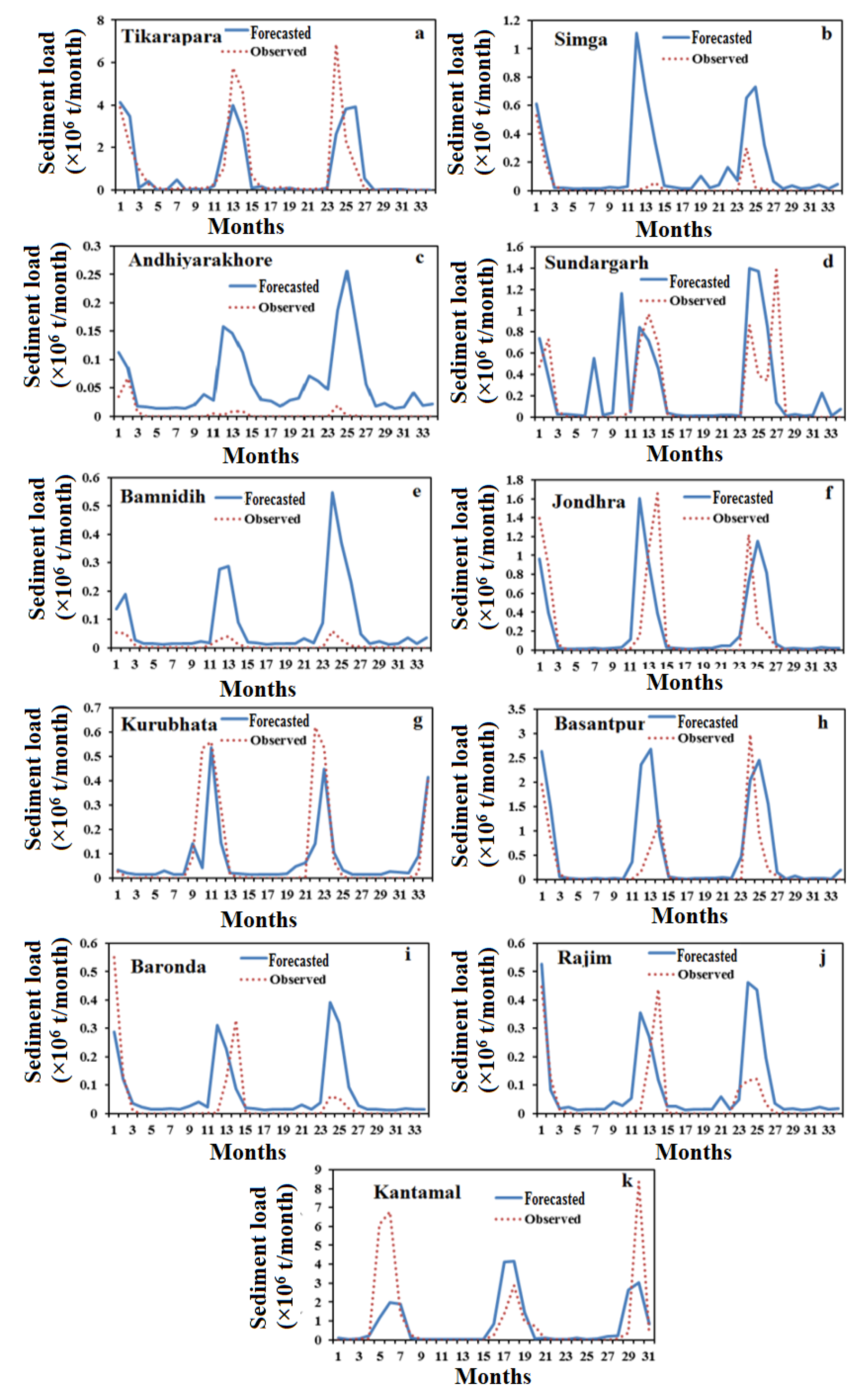
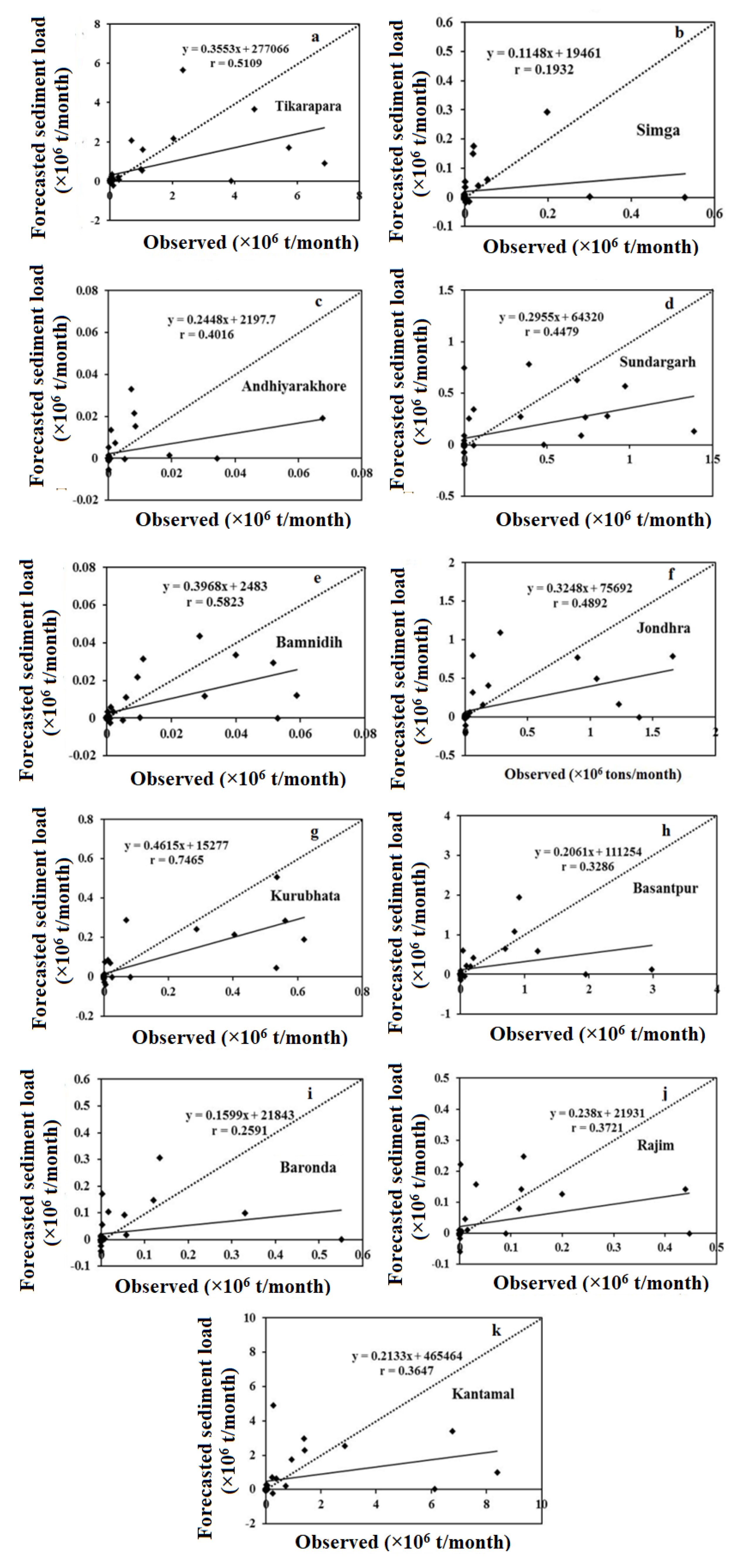
Figure 7 and Figure 8 illustrate the ANN-MOGA-51 model’s hydrologic graph and scatter plot, respectively. The hydrologic graph revealed that, except for the Kantamal, Andhiyarakore, Simga, and Bamnidih stations, the predicted SL corresponds to the observed SL data’s variability. Andhiyarakhore is a small tributary that has a relatively small CA; however, despite its size, it carries a relatively small SL. The reason for this is that relatively small CA basins are unable to store SL and allow for the complete removal of all material that has been eroded. The presence of a large dam named Minimata Bango at Bamnidih is the primary factor that contributes to the modeled output not being accurate. Although Simga has a topography that is almost entirely composed of limestone and a relatively large catchment area, the area is relatively flat. Because of this, the sediment yield and water discharge are relatively low in comparison to those of other tributaries, such as Seonath and Tel, which have a smaller catchment area. Further, its complex non-linear erosion and transportation process of sedimentation resulted in the poor performance of the proposed model at some gauging stations. The high skewness, Kurtosis, coefficient of variation (COV) and maximum/mean value of suspended sediment load indicate its complex and highly erratic behaviours as compared to other variables (water discharge, rainfall and temperature). Thus, estimation of suspended sediment load through mathematical models is very difficult comparative to other variables [24]. The highest coefficient of variation of rainfall is found at Kantamal. This could also explain the corresponding water discharge and the SL dataset’s wide variation and non-normal distribution. Similarly, the ANN-MOGA-51 results are nearer to the bisector line which is also known as the 45 ° line, except for the four gauging stations that were mentioned earlier (Figure 8). The scatter plots and hydrographs show that the magnitudes and medium, high, and low SL forecasted values generated by the best ANN-MOGA-51 forecasting model are also fairly close to the corresponding actual SL values. The ANN-MOGA-51 model displayed a positive value SL at each of the 11 gauge stations, although the SL output was either 0 or very near zero (Figure 7 and Figure 8). Based on these findings, it was determined that the application of ANN in conjunction with GA is the method that yields the most accurate results for calculating SL in the MR basin system. The forecasting model provides the highest level of accuracy at the Tikarapara gauging station compared to any other station gauging station. This may be due to the location of Tikarapara, which is at the most downstream portion of the MR basin and possesses the highest WD, CA, RF, and SL of any of the gauging stations [24,47].

4.3. AR Forecasting Model

In an autoregression model, the SL forecast is generated through a linear combination of the SL time series data. In this study, AR models are developed by the linear combination of previous data of the variable (sediment yield). The AR model is a fundamental class of time series model. It predicts future values by adding up the weighted sums of lagged past data. Various AR models were developed by different input parameter selections with different autoregression of the variable and compared the performances of each other. In this method, the maximum lag selection is considered 12 due to seasonal variation of data and using ACF.
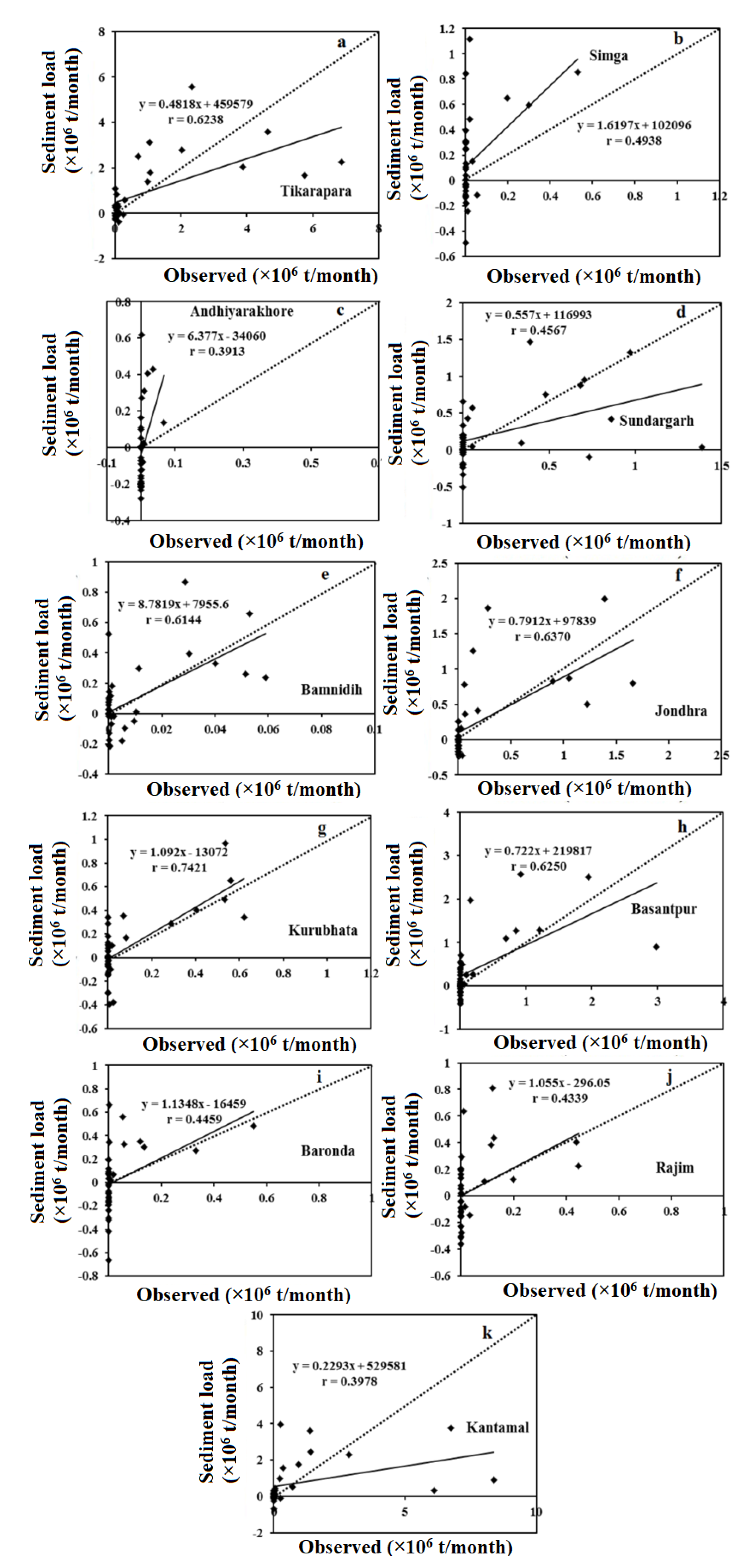
The error statistics of the AR model are given in Table 6. The test dataset’s low MAE and RMSE, as well as its high r value, revealed that the AR forecasting model could justifiably fit the data. The training dataset revealed a similar pattern of behavior, which is not surprising given that the linear model will never be overfitted to the training data. It reveals that the RMSE, MSE, and MAE of training and testing data are trending in the same direction because these are related to one another in a direct proportion, as expected for the linear model. It is observed that this model does not provide satisfactory performance at various gauging stations. The r values are not significant at various gauging stations. Poor correlation is found in all gauging stations except Tikarapara, Kurubhata, and Bamnidih. It is seen in the hydrograph (Figure 9) and scatters plot (Figure 10) that the AR model generates a greater percentage of negative SL values at low SL values as compared to other models. The AR provided the best result at Tikarapara similar to MAR and ANN-MOGA-51 models.

4.4. The Multivariate Autoregressive (MAR) Forecasting Model

The MAR model was designed using training datasets and the combination of the autoregression of multiple factors (WD, RF, SL, and T) as well as spatial variables (CA, RT, and R). The MAR model forecasted a one-step-ahead of the SL value using 51 input parameters (12 from each of the 4 temporal parameters and 3 from the spatial parameters). There is no need for a validation dataset because the linear model does not overfit.
For testing, the same testing data that were applied to the ANN models were used. Table 7 displays the MAR model’s error statistics. During the phases of training and testing, it was observed that the RMSE and MAE are very low, and r is high, demonstrating that the MAR forecasting model can reasonably fit the data. It is observed that Tikarapara shows the highest coefficient of correlation between the actual and forecasted SL values, and Andhiyarakhore station has the lowest correlation coefficient. The proposed model offered the best level of accuracy at the Tikarapara site and the lowest accuracy at Andhiyarakhore.
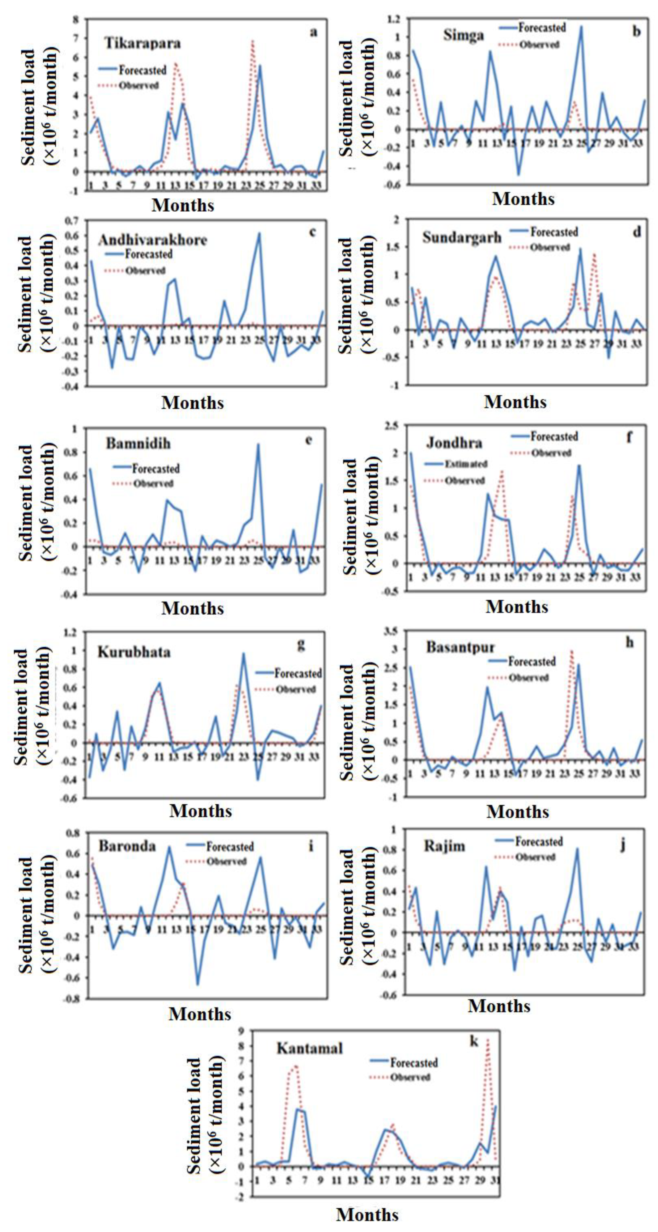
Figure 11 and Figure 12 show the MAR model’s hydrograph and scatter plot. The figure clearly shows that the MAR model presented a negative number where the SL is zero or near zero. It was also realized that the model could not capture low SL as evidenced by the scatter plot, which predicts a negative value in the case of low SL data including all stations. The modeled SL at Bamnidih and Andhiyarakore varies greatly at all peaks and during small SL. However, SL cannot be negative in actuality.
In the scatter plot, it is found that the MAR results are not closer to the bisector line at the Andhiyarakhore and Bamnidih gauging stations. It was noticed that the linear MAR model is unable to handle non-linearity behavior and, as a result, some negative forecasted values of SL are obtained.

4.5. Comparison Results of Forecasting Models

The best hybrid model (ANN-MOGA-51), traditional MAR, and AR models were compared using the same test data. Table 8 shows that the ANN-MOGA-51 model has the least RMSE, variance, MSE, and highest r score when compared to all other comparative models (MAR and AR). This statistical study indicates that the ANN-MOGA-51 model is the best. As a result, when the optimized input variables and associated elements are taken into account, the ANN-MOGA-51 model outperforms both the AR and MAR models. This advantage is due to the selection of optimal of all ANN parameters using the GA. The good performance of the ANN-MOGA-51 model may be attributed to the utilization of time series lag data of SL, RF, T, and WD with spatial data (CA, R and RT), which are more informative by ANN in conjunction with multi-objective GA method and lagged input variable selection using multi-objective GA.
Table 8 demonstrates that the AR model performs the worst due to the highest RMSE, MSE, variance, and lowest r as compared to other models. This worst performance in the AR model is also caused due to the consideration of only SL as the lag time input variable and the exclusion of temporal (WD, T, and RF) and spatial (R, RT, and CA) data. The ANN-MOGA-51 model improved the performance by 12.81% and 10.19% from traditional AR and MAR regression models, respectively. It is also observed from Table 3 and Table 8 that all hybrid intelligence-based models (ANN-MOGA-12, ANN-MOGA-15, ANN-MOGA-48 and ANN-MOGA-51) are providing better results than the traditional regression models (MAR and AR) models on the basis of RMSE and r as performance evaluation criteria.

5. Conclusions

This study revealed the forecasting of SL by the ANN-MOGA-51, MAR, and AR models with a time lag at eleven stations in the MR using various inputs of hydro-climatic factors (RT, RF, T, WD, R, and CA). The input parameters of the SL in the MR were found to be the primary governing factors. The results showed that the ANN-MOGA-51 models performed well and had a higher generalization capability, which was obtained by concurrently optimizing all ANN parameters using the MOGA. As a result, simultaneously optimizing all ANN parameters and input subsets with the MOGA is a better method with satisfactory performance and less computation cost than the traditional grid search and trial-and-error methods. The hydrograph and scatter plots of the ANN-MOGA-51 model also show that the magnitude of the proposed model’s medium, low, and high SL forecasting was closer to the observed values. The best ANN-MOGA-51 model forecasted a positive sediment value even when SL was zero or near zero at all 11 sites in the MR, which is an interesting finding from the hydrograph and scatter plots. On the other hand, MAR and AR models provided negative SL values where SL is low or close to zero. This demonstrated that the data, particularly small, valued samples, exhibit significant non-linear behavior which is not captured by traditional MAR and AR forecasting models.
The results revealed that the hybrid ANN-MOGA model performed significantly better than other traditional MAR and AR models in terms of performance. This is the most appropriate approach because of the relatively better performance and ease of implementation. Thus, the proposed forecasting models are of great assistance to water resource planners and managers because they allow for a better understanding of the problems caused by sedimentation and allow for the finding of alternative solutions to manage the issues in the future by utilizing prior knowledge of forecasting SL. The RF intensity is also an important factor of the SL that is not incorporated in this research due to its unavailability for the improvement of modeling performance but will be considered in future research.

Author Contributions

Conceptualization, A.Y., P.C. and G.V.K.; methodology, A.Y., P.C., A.S. and A.A.; software, G.V.K., P.C. and M.A.A.; validation, A.Y., P.C. and Y.M.; analysis, A.Y., P.C., A.S. and A.A.; investigation, Y.M.; resources, A.S. and M.A.A.; writing—original draft preparation, A.Y., P.C. and A.A.; writing—review and editing, G.V.K., P.C., A.S. and M.A.A.; supervision, A.S., A.A. and Y.M.; project administration, Y.M. All authors have read and agreed to the published version of the manuscript.

Funding

The authors would like to thank the Deanship of Scientific Research at Umm Al-Qura University for supporting this work by Grant Code: (22UQU4330898DSR02).

Institutional Review Board Statement

Not applicable.

Informed Consent Statement

Not applicable.

Data Availability Statement

This study’s data were obtained after a non-disclosure agreement had been signed with the Central Water Commission. The author also thanks the National Institute of Technology, Rourkela, India, for providing the necessary facilities for this study.

Conflicts of Interest

The authors declare no conflict of interest.

References

  1. Frémion, F.; Bordas, F.; Mourier, B.; Lenain, J.; Kestens, T.; Courtin-Nomade, A. Influence of dams on sediment continuity: A study case of a natural metallic contamination. Sci. Total Environ. 2016, 547, 282–294. [Google Scholar] [CrossRef] [PubMed]
  2. Xia, X.; Dong, J.; Wang, M.; Xie, H.; Xia, N.; Li, H.; Zhang, X.; Mou, X.; Wen, J.; Bao, Y. Effect of water-sediment regulation of the Xiaolangdi reservoir on the concentrations, characteristics, and fluxes of suspended sediment and organic carbon in the Yellow River. Sci. Total Environ. 2016, 571, 487–497. [Google Scholar] [CrossRef] [PubMed] [Green Version]
  3. Honorato, A.G.D.S.M.; Silva, G.B.L.D.; Guimarães Santos, C.A. Monthly streamflow forecasting using neuro-wavelet techniques and input analysis. Hydrol. Sci. J. 2018, 63, 2060–2075. [Google Scholar] [CrossRef] [Green Version]
  4. Dutta, S. Soil erosion, sediment yield and sedimentation of reservoir: A review. Model. Earth Syst. Environ. 2016, 2, 123. [Google Scholar] [CrossRef] [Green Version]
  5. Jansson, M.B. Land Erosion by Water in Different Climates; UNGI Report No. 57; Department of Physical Geography, University of Uppsala: Uppsala, Sweden, 1982. [Google Scholar]
  6. Syvitski, J.P.M.; Peckham, S.D.; Hilberman, R.; Mulder, T. Predicting the Terrestrial Flux of Sediment to the Global Ocean: A Planetary Perspective. Sediment. Geol. 2003, 162, 5–24. [Google Scholar] [CrossRef]
  7. Gupta, H.; Chakrapani, G.J. Temporal and spatial variations in water flow and sediment load in Narmada River Basin, India: Natural and man-made factors. Environ. Geol. 2005, 48, 579–589. [Google Scholar] [CrossRef]
  8. Ramesh, R.; Subramanian, V. Temporal, spatial and size variation in the sediment transport in the Krishna River basin, India. J. Hydrol. 1988, 98, 53–65. [Google Scholar] [CrossRef]
  9. Bastia, F.; Equeenuddin, S.M. Spatio-temporal variation of water flow and sediment discharge in the Mahanadi River, India. Glob. Planet. Chang. 2016, 144, 51–66. [Google Scholar] [CrossRef]
  10. Thodsen, H.; Hasholt, B.; Kjarsgaard, J.H. The influence of climate change on suspended sediment transport in Danish rivers. Hydrol. Process. 2008, 22, 764–774. [Google Scholar] [CrossRef]
  11. Merritt, W.S.; Letcher, R.A.; Jakeman, A.J. A review of erosion and sediment transport models. Environ. Model. Softw. 2003, 18, 761–799. [Google Scholar] [CrossRef]
  12. Salas, J.D.; Delleur, J.W.; Yevjevich, V.; Lane, W.L. Applied Modeling of Hydrologic Time Series; Water Resources Publications: Littleton, CO, USA, 1980; 484p. [Google Scholar]
  13. Adamowski, J.; Chan, H.F.; Prasher, S.O.; Ozga-Zielinski, B.; Sliusarieva, A. Comparison of multiple linear and nonlinear regression, autoregressive integrated moving average, artificial neural network, and wavelet artificial neural network methods for urban water demand forecasting in Montreal, Canada. Wat. Resour. Res. 2012, 48, W01528. [Google Scholar] [CrossRef]
  14. Pektas, A.O.; Cigizoglu, H.K. Long-range forecasting of suspended sediment. Hydrol. Sci. J. 2017, 62, 2415–2425. [Google Scholar] [CrossRef]
  15. Partal, T.; Cigizoglu, H.K. Estimation and forecasting of daily suspended sediment data using wavelet-neural networks. J. Hydrol. 2008, 358, 317–331. [Google Scholar] [CrossRef]
  16. Nourani, V.; Alizadeh, F.; Roushangar, K. Evaluation of a two-stage SVM and spatial statistics methods for modeling monthly river suspended sediment load. Water Resour. Manag. 2016, 30, 393–407. [Google Scholar] [CrossRef]
  17. Meshram, S.G.; Ghorbani, M.A.; Deo, R.C.; Kashani, M.H.; Meshram, C.; Karimi, V. New approach for sediment yield forecasting with a two-phase feedforward neuron network-particle swarm optimization model integrated with the gravitational search algorithm. Water Resour. Manag. 2019, 33, 2335–2356. [Google Scholar] [CrossRef]
  18. ASCE. Task Committee on Application of Artificial Neural Networks in Hydrology Artificial neural networks in hydrology. I: Preliminary concepts. J. Hydrol. Eng. 2000, 5, 115–123. [Google Scholar] [CrossRef]
  19. Reddy, P.V.B. Modelling and Optimization of Wire Electrical Discharge Machining of Cr-Mo-V Special Alloy Steel Using Neuro Genetic Approach. Ph.D. Thesis, Jawaharlal Nehru Technological University, Anantapur, India, 2014. [Google Scholar]
  20. Tokar, A.S.; Johnson, P.A. Rainfall-Runoff Modelling using Artificial Neural Networks. J. Hydrol. Eng. 1999, 4, 232–239. [Google Scholar] [CrossRef]
  21. Dawson, C.W.; Harpham, C.; Wilby, R.L.; Chen, Y. An evaluation of artificial neural network techniques for flow forecasting in the river Yangtze, China. Hydrol. Earth Syst. Sci. 2002, 6, 619–626. [Google Scholar] [CrossRef]
  22. Kar, A.K.; Lohani, A.K.; Goel, N.K.; Roy, G.P. Development of Flood Forecasting System Using Statistical and ANN Techniques in the Downstream Catchment of Mahanadi Basin, India. J. Water Resour. Prot. 2010, 2, 880–887. [Google Scholar]
  23. Bishop, M. Neural Networks for Pattern Recognition; Clarendon Press: Oxford, UK, 1998. [Google Scholar]
  24. Yadav, A.; Chatterjee, S.; Equeenuddin, S.M. Suspended Sediment Yield Estimation using Genetic Algorithm-based Artificial Intelligence Models in Mahanadi River. Hydrol. Sci. J. 2018, 63, 1162–1182. [Google Scholar] [CrossRef]
  25. Holland, J. Adaptation in Natural and Artificial Systems; The University of Michigan Press: Ann Arbor, MI, USA, 1975. [Google Scholar]
  26. Hosseini, S.A.; Abbaszadeh Shahri, A.; Asheghi, R. Prediction of bedload transport rate using a block combined network structure. Hydrol. Sci. J. 2022, 67, 117–128. [Google Scholar] [CrossRef]
  27. Chatterjee, S.; Bandopadhyay, S. Reliability estimation using a genetic algorithm-based artificial neural network: An application to a load-haul-dump machine. Expert Syst. Appl. 2012, 39, 10943–10951. [Google Scholar] [CrossRef]
  28. Asheghi, R.; Hosseini, S.A.; Saneie, M.; Shahri, A.A. Updating the neural network sediment load models using different sensitivity analysis methods: A regional application. J. Hydroinformatics 2020, 22, 562–577. [Google Scholar] [CrossRef] [Green Version]
  29. Adib, A.; Mahmoodi, A. Prediction of Suspended Sediment Load using ANN GA Conjunction Model with Markov Chain Approach at Flood Conditions. KSCE J. Civ. Eng. 2016, 1, 447–457. [Google Scholar] [CrossRef]
  30. Chatterjee, S.; Bandopadhyay, S. Goodnews Bay Platinum Resource Estimation Using Least Squares Support Vector Regression with Selection of Input Space Dimension and Hyperparameters. Nat. Resour. Res. 2016, 20, 117–129. [Google Scholar] [CrossRef]
  31. Samarasinghe, S. Neural Networks for Applied Sciences and Engineering: From Fundamentals to Complex Pattern Recognition; CRC Press: Boca Raton, FL, USA, 2016; p. 555. [Google Scholar]
  32. Geman, S.; Bienenstock, E.; Doursat, R. Neural networks and the bias/variance dilemma. Neural Comput. 1992, 4, 1–58. [Google Scholar] [CrossRef]
  33. Rosales-Perez, A.; Escalante, H.J.; Gonzalez, J.A.; Reyes-Garcia, C.A. Bias and variance optimization for SVMs model selection. In Proceedings of the Twenty-Sixth International FLAIRS Conference, St. Pete Beach, FL, USA, 22–24 May 2013. [Google Scholar]
  34. Kulasiri, D.; Verwoerd, V. Stochastic Dynamics: Modeling Solute Transport in Porous Media; North Holland Series in Applied Mathematics and Mechanics; Elsevier: Amsterdam, The Netherlands, 2002; p. 44. [Google Scholar]
  35. Levin, S.A. Population dynamics in models in heterogeneous environments. Annu. Rev. Ecol. Syst. 1976, 7, 287. [Google Scholar] [CrossRef]
  36. Deb, K.; Pratap, A.; Agarwal, S.; Meyarivan, T. A fast and elitist multi-objective genetic algorithm: NSGA-II. IEEE Trans. Evol. Comput. 2002, 6, 181–197. [Google Scholar] [CrossRef] [Green Version]
  37. Bharti, P.S.; Maheshwari, S.; Sharma, C. Multi-objective optimization of electric-discharge machining process using controlled elitist NSGA-II. J. Mech. Sci. Technol. 2012, 26, 1875–1883. [Google Scholar] [CrossRef]
  38. Behzadian, K.; Kapelan, Z.; Savic, D.; Ardeshir, A. Stochastic sampling design using multi-objective genetic algorithm and adaptive neural network. Environ. Model. Softw. 2009, 24, 530–541. [Google Scholar] [CrossRef] [Green Version]
  39. Zhou, C.C.; Yin, G.F.; Hu, X.B. Multi-objective optimization of material selection for sustainable products: Artificial neural networks and genetic algorithm approach. Mater. Des. 2009, 30, 1209–1215. [Google Scholar] [CrossRef]
  40. Yadav, A.; Chatterjee, S.; Equeenuddin, S.M. Suspended sediment yield modeling in Mahanadi River, India by multi-objective optimization hybridizing artificial intelligence algorithms. Int. J. Sediment Res. 2021, 36, 76–91. [Google Scholar] [CrossRef]
  41. Sakai, K.; Osawa, K.; Yoshinaga, A. Development of suspended sediment concentration analysis model and its application with multi-objective optimization. Paddy Water Environ. 2005, 3, 201–209. [Google Scholar] [CrossRef]
  42. Peng, Y.; Ji, C.; Gu, R. Multiobjective optimization model for coordinatec regulation of water flow and sediment in cascade reservoirs. Water Resour. Manag. 2014, 28, 4019–4033. [Google Scholar] [CrossRef]
  43. Cigizoglu, H.K.; Kisi, O. Methods to improve the neural network performance in suspended sediment estimation. J. Hydrol. 2006, 317, 221–238. [Google Scholar] [CrossRef]
  44. Cigizoglu, H.K.; Alp, M. Generalized regression neural network in modelling river sediment yield. Adv. Eng. Softw. 2006, 37, 63–68. [Google Scholar] [CrossRef]
  45. Piotrowski, A.P.; Napiorkowski, M.J.; Napiorkowski, J.J.; Osuch, M. Comparing various artificial neural network types for water temperature prediction in rivers. J. Hydrol. 2015, 529, 302–315. [Google Scholar] [CrossRef]
  46. Kant, A.; Suman, P.K.; Giri, B.K.; Tiwari, M.K.; Chatterjee, C.; Nayak, P.C.; Kumar, S. Comparison of multi-objective evolutionary neural network, adaptive neuro-inference system and bootstrap-based neural network for flood forecasting. Neural Comput. Appl. 2013, 23, S231–S246. [Google Scholar] [CrossRef]
  47. India-WRIS. Water Resources Information System of India. Available online: http://india-wris.nrsc.gov.in/wrpinfo/index.php?title=Mahanadi (accessed on 8 August 2016).
  48. Yadav, A.; Chatterjee, S.; Equeenuddin, S.M. Prediction of Suspended Sediment Yield by Artificial Neural Network and Traditional Mathematical Model in Mahanadi River Basin, India. J. Sustain. Water Resour. Manag. 2017, 4, 745–759. [Google Scholar] [CrossRef]
  49. Rojas, R. Neural Network: A Systematic Introduction; Springer: Berlin, Germany, 1996; pp. 151–184. [Google Scholar]
  50. Hagan, M.T.; Menhaj, M.B. Training feedforward networks with the Marquardt algorithm. IEEE Trans. Neural Netw. 1994, 5, 989–993. [Google Scholar] [CrossRef]
  51. Ebtehaj, I.; Bonakdari, H.; Safari, M.J.S.; Gharabaghi, B.; Zaji, A.H.; Madavar, H.R.; Khozani, Z.S.; Es-haghi, M.S.; Shishegaran, A.; Mehr, A.D. Combination of sensitivity and uncertainty analyses for sediment transport modeling in sewer pipes. Int. J. Sediment Res. 2020, 35, 157–170. [Google Scholar] [CrossRef]
  52. Riahi-Madvar, H.; Gharabaghi, B. Pre-processing and Input Vector Selection Techniques in Computational Soft Computing Models of Water Engineering. In Computational Intelligence for Water and Environmental Sciences; Springer: Singapore, 2022; pp. 429–447. [Google Scholar]
  53. Dehghani, M.; Seifi, A.; Riahi-Madvar, H. Novel forecasting models for immediate-short-term to long-term influent flow prediction by combining ANFIS and grey wolf optimization. J. Hydrol. 2019, 576, 698–725. [Google Scholar] [CrossRef]
  54. Riahi-Madvar, H.; Dehghani, M.; Memarzadeh, R.; Gharabaghi, B. Short to long-term forecasting of river flows by heuristic optimization algorithms hybridized with ANFIS. Water Resour. Manag. 2021, 35, 1149–1166. [Google Scholar] [CrossRef]
  55. Riahi-Madvar, H.; Seifi, A. Uncertainty analysis in bed load transport prediction of gravel-bed rivers by ANN and ANFIS. Arab. J. Geosci. 2018, 11, 1–20. [Google Scholar] [CrossRef]
  56. Gowda, C.C.; Mayya, S.G. Comparison of back propagation neural network and genetic algorithm neural network for stream flow prediction. J. Comput. Environ. Sci. 2014, 290127. [Google Scholar] [CrossRef] [Green Version]
  57. Senthil Kumar, A.R.; Sudheer, K.P.; Jain, S.K.; Agarwal, P.K. Rainfall-runoff modelling using artificial neural networks: Comparison of network types. Hydrol. Process. Int. J. 2005, 19, 1277–1291. [Google Scholar] [CrossRef]
  58. Ghosh, A.; Das, M.K. Non-dominated rank-based sorting genetic algorithms. Fundam. Inform. 2008, 83, 231–252. [Google Scholar]
  59. Moriasi, D.N.; Arnold, J.G.; Van Liew, M.W.; Bingner, R.L.; Harmel, R.D.; Veith, T.L. Model Evaluation Guidelines for Systematic Quantification of Accuracy in Watershed Simulations. Trans. ASABE 2007, 50, 885–900. [Google Scholar] [CrossRef]
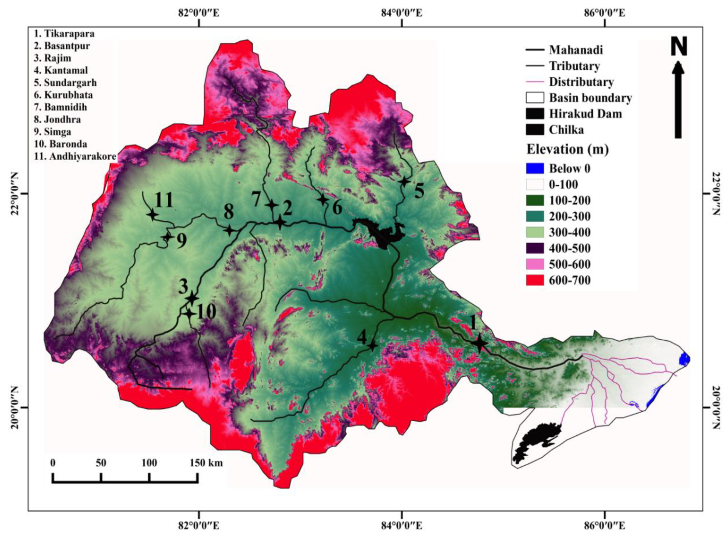
Figure 1. The elevation map of the Mahanadi River basin with the geographical location of 11 gauging stations [48].
Water 15 00522 g001
Figure 2. Flow chart of proposed hybrid ANN-MOGA model for SL forecasting.
Water 15 00522 g002
Figure 3. Spatial variation of monthly average hydro-climatic and geomorphological data such as water discharge (cms) (m3/s), temperature (°C), rainfall (mm) and sediment load (t/ month), relief (m), and catchment area (km2).
Water 15 00522 g003
Figure 4. Comparative analysis of long-term variation over the past two decades of (a) WD, (b) RF, (c) SL, and (d) T.
Water 15 00522 g004
Figure 5. The autocorrelation function (ACF) for monthly hydro-climatical data (a) SL, (b) WD, (c) RF, (d) T.
Water 15 00522 g005
Figure 6. (a) Dilemma between the bias and variance objectives. (b) Variation of individuals and distance. (c) Variation of individuals and corresponding ranking. (d) Generation-wise variation of average spreads of Pareto.
Water 15 00522 g006
Figure 7. Comparison of the actual and forecasted SL during the testing phase of the ANN-MOGA-51 forecasting model (ak).
Water 15 00522 g007
Figure 8. Scatter plot of the actual and forecasted SL of the ANN-MOGA-51 forecasting model during the testing phase (ak).
Water 15 00522 g008
Figure 9. Comparison of the actual and forecasted SL during the testing phase of the AR forecasting model (ak).
Water 15 00522 g009
Figure 10. Scatter plot of the actual and forecasted SL of the AR forecasting model during the testing phase (ak).
Water 15 00522 g010
Figure 11. Comparison of the actual and forecasted SL during the testing phase of the MAR forecasting model (ak).
Water 15 00522 g011
Figure 12. Scatter plot of the actual and forecasted SL of the MAR forecasting model during the testing phase (ak).
Water 15 00522 g012
Table 1. Spearman rank correlation coefficient ® of hydro-climatolic data from eleven stations for the MR.
Stationsr1
(WD-SL)
r2
(SL-RF)
r3
(SL-T)
Tikarapara0.8919515790.6675660990.167164223
Sundargarh0.9331626430.7194900120.083275757
Simga0.9121711570.6691449680.016117111
Jondhara0.9536150620.6347880840.024002708
Andhiyarakhore0.9304409840.6794836790.172300271
Kurubhata0.9147905310.7395417860.09457768
Bamnidih0.7929755740.6738000750.19294038
Rajim0.9335154520.652771319−0.053703323
Kantamal0.7848582550.6535823430.045884228
Baronda0.8961285530.7188656030.170015607
Basantpur0.9002612370.7177222360.120971863
Table 2. Various multi-objective GA-based ANN models using different input variables with lags.
ModelsNumber of Initial Inputs Input Parameters
ANN-MOGA-5151SL, WD, RF, T, RT, R and CA
ANN-MOGA-4848SL, WD, RF and T
ANN-MOGA-1515SL, RT, R and CA
ANN-MOGA-1212SL
Table 3. Performance comparison of the hybrid multi-objective GA-based ANN forecasting models in the testing phase.
ModelsRMSEInitially Inputs No.MSEMAEVARr
ANN-MOGA-510.011639510.0001350.0038020.0001360.643313
ANN-MOGA-480.013343480.0001780.003811940.00017830.5674853
ANN-MOGA-150.013637150.0001860.00440.0001860.513217
ANN-MOGA-120.01181120.0001390.0036260.000140.623344
Table 4. Optimally selected parameters of ANN-MOG models.
ModelsTransfer FunctionNeuronsInputsµ
ANN-MOGA-51Log-sigmoid, pure linear29222
ANN-MOGA-48Tan-sigmoid, pure linear19219
ANN-MOGA-15Pure linear, tan-sigmoid151010
ANN-MOGA-12Tan-sigmoid, pure linear466
Table 5. Error statistics of ANN-MOGA-51 forecasting model during validation, testing, and training phase.
ANN-MOGA-51MSERMSErError VarianceMAE
Training0.0002410.0155260.6689380.0002410.004677
Validation5.25 × 10−50.0072430.77305.26 × 10−50.002867
Testing0.0001350.0116390.6433130.0001360.003802
Tikarapara0.0003960.0199050.7310510.0004070.010517
Simga1.17 × 10−50.0034220.59309.81 × 10−60.001707
Andhiyarakhore1.10 × 10−50.0033190.40019.06 × 10−50.001749
Sundargarh2.60 × 10−50.0050970.6352.67 × 10−50.002466
Bamnidih3.33 × 10−50.0057690.6953.27 × 10−50.002765
Jondhara3.02 × 10−50.0054990.7372.91 × 10−50.002534
Kurubhata2.06 × 10−50.0014340.9141.97 × 10−60.000865
Basantpur0.0002290.0151210.4781430.0002220.006185
Baronda5.66 × 10−60.0023790.4955.23 × 10−60.001319
Rajim2.10 × 10−60.0014480.6692.15 × 10−60.000722
Kantamal0.0008060.0283950.6595180.0008010.01198
Table 6. Error statistics of the autoregressive (AR) forecasting model at different gauging stations.
ARRMSEMSEMAEVARr
Training0.016400.000270.004730.000270.61268
Testing0.013350.000180.003650.000180.49670
Tikarapara0.025760.000660.011190.000660.51087
Simga0.001853.42 × 10−60.000693.49 × 10−060.19322
Andhiyarakhore0.000204.07 × 10−89.30×10−54.15 × 10−080.40166
Sundargarh0.005553.08 × 10−50.003033.02 × 10−050.44791
Bamnidih0.000245.56 × 10−80.000125.46 × 10−080.58226
Jondhara0.006684.46 × 10−50.003234.48 × 10−050.48917
Kurubhata0.002224.92 × 10−60.001034.72 × 10−060.74650
Basantpur0.010590.000110.004110.000110.32857
Baronda0.001873.49 × 10−60.000733.56 × 10−60.25906
Rajim0.001773.14 × 10−60.000793.18 × 10−60.37205
Kantamal0.033860.001150.014810.001160.36473
Table 7. Error statistics of single forecasting MAR model at each station.
MARMAEVARrMSERMSE
Training0.006400.000230.680100.000230.01516
Testing0.005620.000170.556200.000170.01296
Tikarapara0.013060.000540.623800.000520.02284
Simga0.003952.65×10−50.493802.99×10−50.00547
Andhiyarakhore0.002601.20×10−50.391301.16×10−50.00341
Sundargarh0.004864.91×10−50.456704.79×10−50.00692
Bamnidih0.002721.53×10−50.614401.66×10−50.00407
Jondhara0.004585.44×10−50.637005.36×10−50.00732
Kurubhata0.002281.01×10−50.742109.80×10−60.00313
Basantpur0.006100.000100.625000.000110.01025
Baronda0.003061.75×10−50.445901.70×10−50.00412
Rajim0.003091.64×10−50.433901.59×10−50.00398
Kantamal0.016520.001110.397800.001080.03292
Table 8. Statistical performance evaluation of ANN-MOGA-51, AR, and MAR models along with all gauging stations in a testing phase.
ModelsANN-MOGA-51MARAR
StatisticsRMSErRMSErRMSEr
Testing0.011640.64330.012960.55620.013350.4967
Tikarapara0.019910.73110.022840.62380.025760.5109
Simga0.003420.59300.005470.49380.001850.1932
Andhiyarakhore0.003320.40010.003410.39130.000200.4017
Sundargarh0.005100.63500.006920.45670.005550.4479
Bamnidih0.005770.69500.004070.61440.000240.5821
Jondhara0.005500.73700.007320.63700.006680.4892
Kurubhata0.001430.91400.003130.74210.002220.7465
Basantpur0.015120.47810.010250.62500.010590.3286
Baronda0.002380.49500.004120.44590.001870.2591
Rajim0.001450.66900.003980.43390.001770.3721
Kantamal0.028400.65950.032920.39780.033860.3647
Disclaimer/Publisher’s Note: The statements, opinions and data contained in all publications are solely those of the individual author(s) and contributor(s) and not of MDPI and/or the editor(s). MDPI and/or the editor(s) disclaim responsibility for any injury to people or property resulting from any ideas, methods, instructions or products referred to in the content.