Article

Supplementing Missing Data Using the Drainage-Area Ratio Method and Evaluating the Streamflow Drought Index with the Corrected Data Set

by
Evren Turhan
* and
Serin Değerli Şimşek
Department of Civil Engineering, Adana Alparslan Türkeş Science and Technology University, Adana 01250, Turkey
*
Author to whom correspondence should be addressed.
Water 2023, 15(3), 425; https://doi.org/10.3390/w15030425
Submission received: 12 December 2022 / Revised: 9 January 2023 / Accepted: 16 January 2023 / Published: 20 January 2023
(This article belongs to the Special Issue Assessment and Management of Hydrological Risks Due to Climate Change)

Abstract

:
In water resources management, it is essential to have a full and complete set of hydrological parameters to create accurate models. Especially for long-term data, any shortcomings may need to be filled using the appropriate methods. Moving the recorded observed data using the drainage-area ratio (DAR) method to different points is considered one of these methods. The present study used data from six different flow observation stations in the Asi River sub-basin, known as the fertile agricultural areas in Turkey, and transferred the data to various other locations that already have existing observations. This study tested how close the values this method produced were to the actual values and investigated the question “how is missing data imputation improved by the determination of method bias coefficients?” to analyze the method’s accuracy, the streamflow drought index (SDI)—a hydrological drought index—was applied over a 12 month timescale. Contour maps were formed according to both the obtained index results by using the original data from the target station and the transferred streamflow data. As a result of this study, a severe divergence from the actual values was observed in the data directly transferred to the target stations in proportion to their area. The distance of the existing stations between each other produced a very high correlation coefficient, both in the direct transfer process and after the correction was applied. Similarly, in terms of drought index calculations, values close to 97% were seen in the original and transferred flow rates. Consequently, from the perspective of the effective management processes of water resources, the transportation of the data from basin-based observation stations corrected according to the drainage areas can be thought to positively affect the design stages and cost calculations for future water structures.

1. Introduction

Water is vitally important for living things on Earth. From the past to the present, issues such as the efficient use of water resources, flood control and protection from all kinds of natural disasters have been accepted as primary problems to be solved. Any water source used for drinking water and agricultural purposes may also meet the needs for hydroelectricity, water storage, water supply and water transportation. Therefore, streamflow data are often used to design and operate hydraulic structures in accordance with their purpose [1,2,3]. Considering the planning and design processes, it is critical that past data are not missing. However, it is a fact that it is difficult and costly to perform these measurements for each point in a basin. There may be data that are missing or that could not be measured for a variety of reasons, including climate conditions, transportation difficulties or problems in the measuring device [2,4,5,6]. Many studies have been carried out and different methods investigated to complete these missing ones. Recently, artificial intelligence techniques and statistical studies are frequently used to complete the missing flow data in the literature [2,4,5,6,7,8,9]. These data can be completed appropriately by various statistical methods [10]. Accordingly, studies on the transfer of existing data to other measurement locations have researched the use of the drainage-area ratio (DAR) method [11,12,13,14,15,16,17]. This method refers to the transfer of streamflow gauge station (SGS) data to a different SGS according to the ratio of their areas. The DAR method is mostly used to complete missing data or analyze the accuracy of measured data. Completing the missing streamflow data using the proper methods will make significant contributions to the structural measures to be taken against natural disasters, such as flood and drought. Within the scope of hydrology studies, flood discharge values are calculated by statistical and deterministic methods for different return periods, such as 2, 5, 10, 25, 50, 100, 200, 500, 1000 and 10,000 years [18,19]. These discharge values can also be calculated by empirical formulas, such as the McMath and rational methods. In addition, hydrological analogy methods are among the other solution options considered for peak streamflow predictions [20]. It is quite significant that the streamflow values are complete in terms of drought works. Population growth, urbanization, trends in water use and environmental differences have increased the drought effect in recent years. To minimize the devastating effects of drought, there are many drought analysis studies that have been performed on a regional basis, especially in the Asi River basin. In most of these studies, it has been stated that severe droughts were seen after the 2000s [21,22,23,24,25]. The streamflow drought index (SDI) is one of the drought analysis indexes suggested by Nalbantis (2008) [26]. In this method, only the average streamflow values are used as input data, and the drought’s temporal and spatial changes can be investigated with the obtained SDI values [27,28,29,30]. Within this study’s scope, the lower smaller Asi River sub-basin borders, which contain the essential agricultural areas of Turkey, were selected as the study area. In Turkey, six different SGSs, numbered D19A026, D19A027, D19A028, D19A030, 1906 and 1907, which belong to the Electricity Works Survey Administration (known as EIEI) and the State Hydraulic Works (known as DSI) institutions, were used. The average monthly streamflow data in the years from 2000 to 2011 were preferred for the analysis of the accuracy of the DAR method. Station data from D19A026, D19A027, D19A028 and D19A030 were transferred to stations 1906 and 1907 at different locations. This was conducted to appropriately compensate for any missing data due to the lack of recorded data from the 1906 and 1907 SGSs after 2011 in case any water structure planning was required in these regions in the future. As a result, considering the available information, the hydrological drought index values, based on 12 year streamflow data, were calculated within the scope of this study, and the effect of the data introduced by the DAR method on these calculations was examined. This study explored the error rate or deviation values between the original and the transferred data, as well as their convergence with the existing data. In cases where the SGS data were not available, it was thought that completing the deficiencies with the help of this method may contribute to the prevention of possible errors, especially in the design processes of new water structures.

2. Materials and Methods

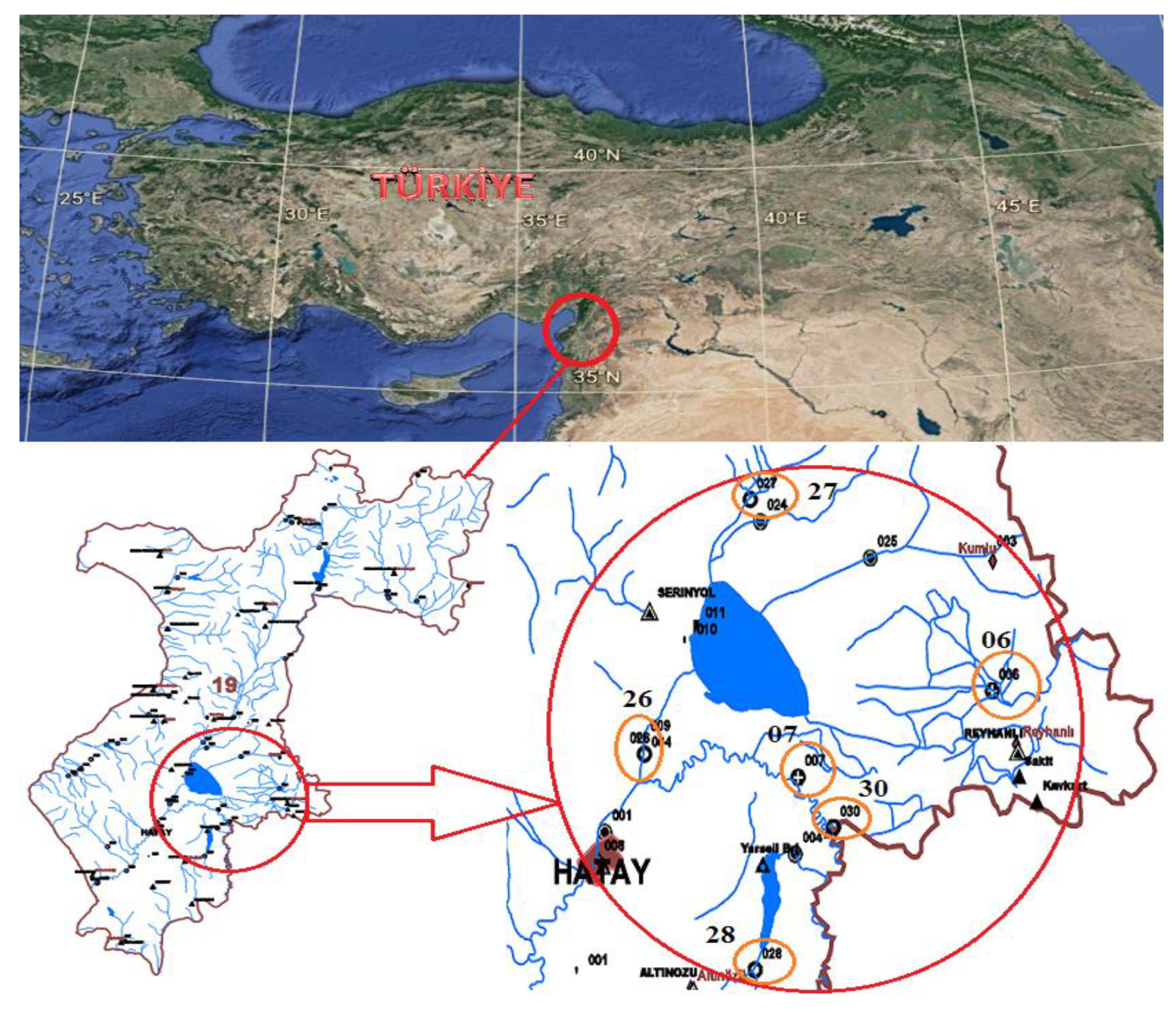
2.1. Study Area and Data Used

In total, there are 25 main basins in Turkey. The Asi River basin is included in these basins and is referred to as the number 19 basin. The basin is between a 36°00′ and 36°08′ North latitudinal line and between a 35°54′ to 36°04′ East longitudinal line in the southern part of Turkey (Figure 1).
The Asi River basin is a transboundary basin with an area of approximately 24.660 km2, where 69% is in Syria, 23% is in Turkey and 8% is in Lebanon [31]. Eighty-eight kilometers of the Asi River flows within the borders of Turkey. At the same time, the Asi River, which irrigates the Amik Plain, changes its south to north directional flow on the Amik Plain and forms a route in a westerly direction. Near the city of Antakya, the flow enters a narrow strait in the east to west direction and forms the Harbiye waterfalls. Later, it forms a delta 6 km southwest of Samandağ, located east of Antakya, and then flows into the Mediterranean. The Asi River was named “Asi or Orontes” (meaning rebellious/insurgent in Turkish) because it flows northwards, unlike the other rivers in the region [32].
In terms of climate, it is in a Mediterranean climate zone, as the summers are hot and dry, and the winters are warm and rainy. However, the climate becomes continental as one moves toward the inner parts of the basin. The Asi River basin is considered one of the most important basins, since it has a drainage area of approximately 7800 km2 and is bordered by neighboring countries [24].
Figure 1. General location of the lower small Asi River sub-basin and streamflow gauge stations (SGSs) [33].
Water 15 00425 g001
In the present study, monthly average streamflow data were used from the SGSs numbered D19A026, D19A027, D19A028, D19A030, 1906 and 1907, located in the lower small Asi River sub-basin. Information on the SGSs used in this study is shown in Table 1.

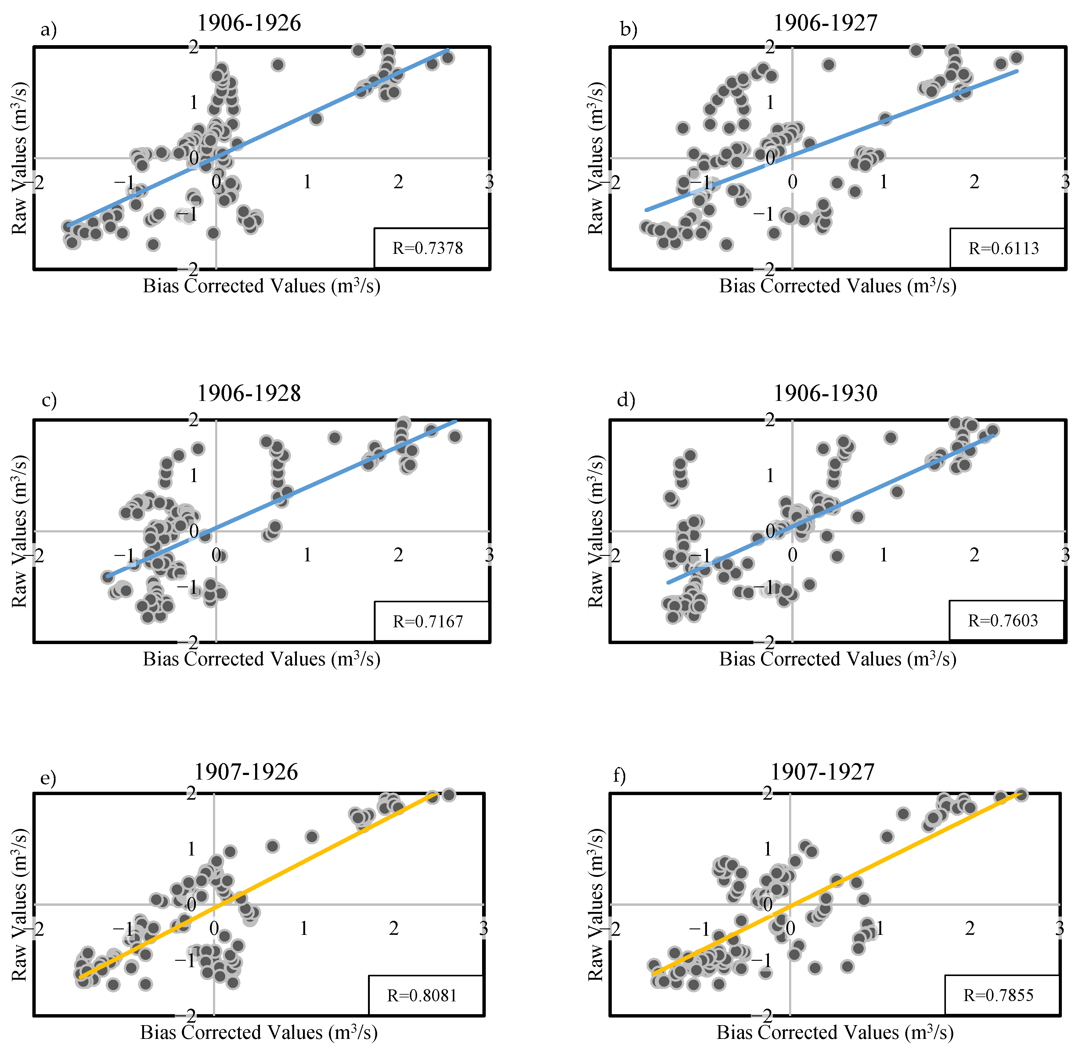
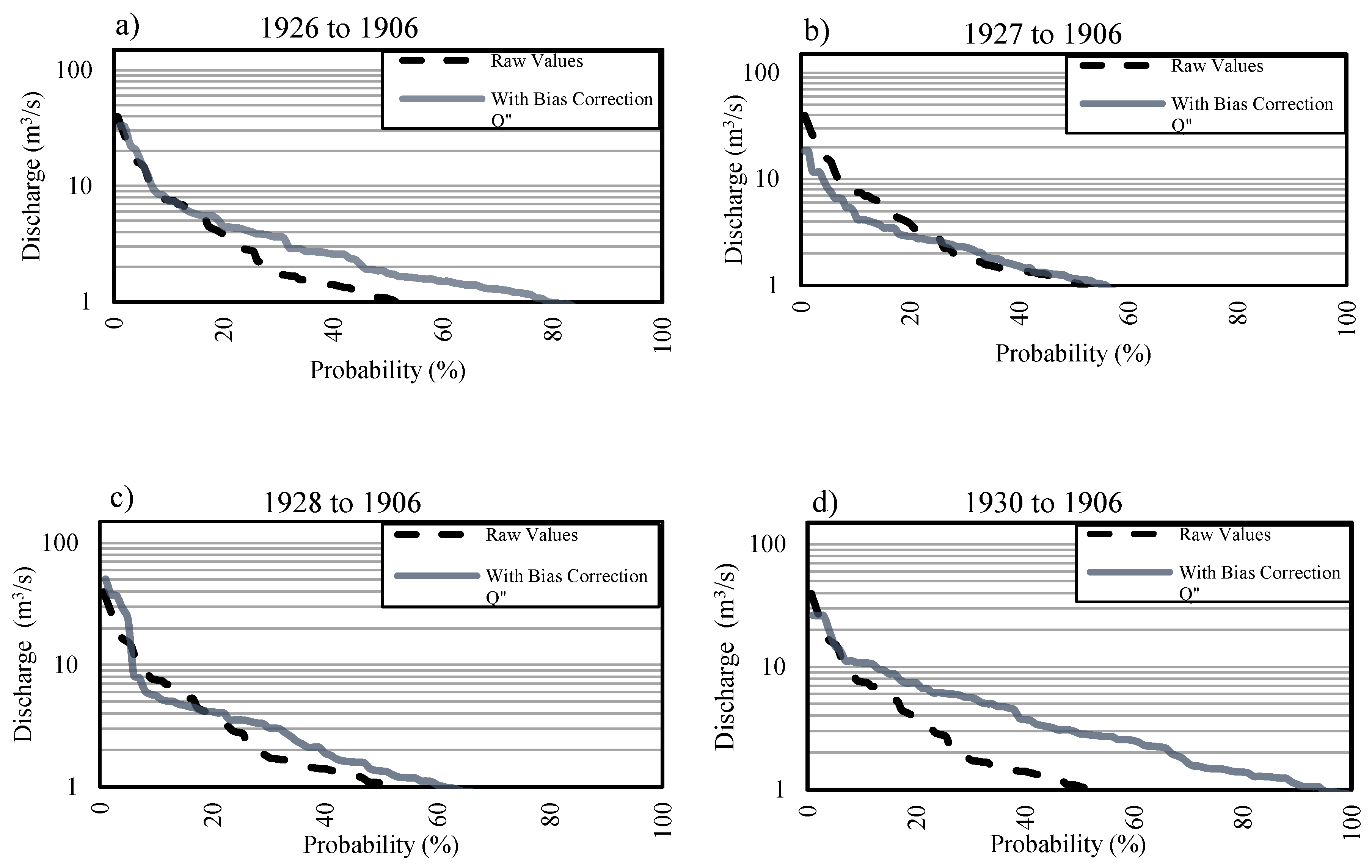
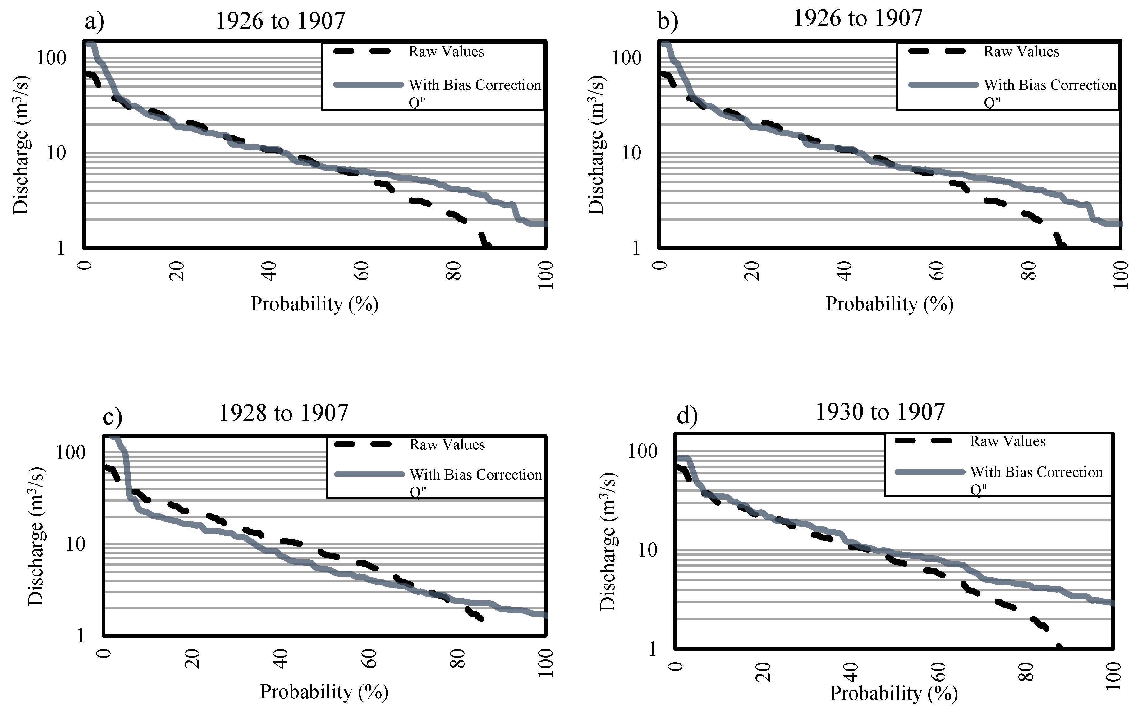
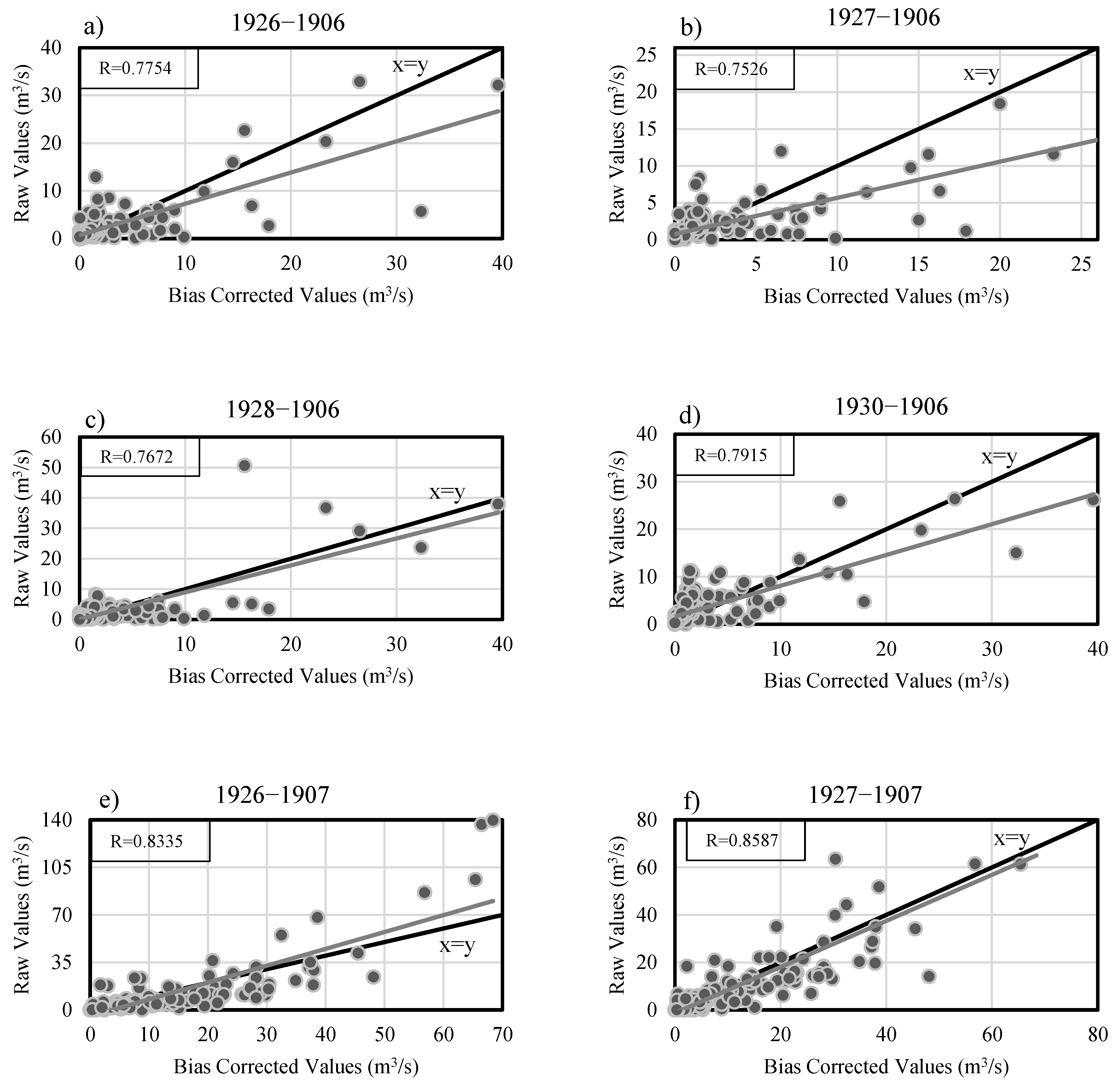
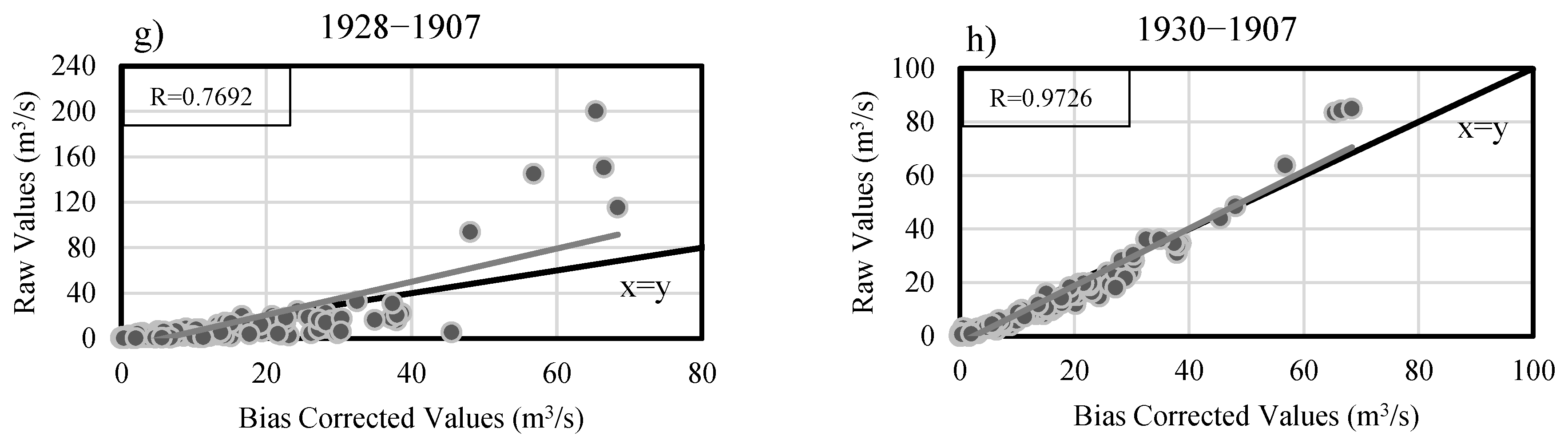
2.2. Drainage-Area Ratio Method

The drainage-area ratio (DAR) method refers to the transfer of the SGS data located in the same basin to another SGS designated point [14,16]. To use this method, it is essential to determine the ϕ and K coefficients obtained from the SGSs in the basin. Basically, only the days in which no flow record at any measuring station were selected. These were divided into calibration data and test data. The K and ϕ coefficients were determined using the calibration data. The test flow rates were calculated with such calibrated data. The accuracy was evaluated graphically and using statistical indicators. Only after such verification was the method calibrated in this way applied to the truly missing data. In general, the formula Q = K. A ϕ is used in this method. In the formula, Q is in m3/s and expresses the daily, monthly or annual flow amount; A is in km2 and represents the drainage area around the selected location. The symbol ϕ is the exponent, and K is the correction coefficient. For example, if there is an SGS at a point i on the stream, the area of this SGS is Ai, and its measured flow is Qi. If the basin drainage area of the location j, where the data will be transported, is evaluated as Aj and its flow rate as Qj, Equations (1) and (2) can be written as follows [15]:
Q i = K i ( A i A j ) ϕ
Q j = K j ( A j A i ) ϕ Q i
To use the method in these operations without bias correction, it is seen that the ϕ exponent and K correction coefficients in the formula take the value of 1 (ϕ = 1, K = 1) [17]. When using the correction, the exponential numbers for ϕ in the equation are calculated, the arithmetic average of the obtained values is taken, and a single value is reached. The formulas used are seen in Equations (3) and (4) [34]:
ϕ a i = l o g ( Q i a / Q j a ) l o g ( A i / A j )
ϕ ¯ = 1 n a = 1 n ϕ a
where n is the number of samples, and “a” represents the flow values in the row and ϕ for that row. To minimize the errors, the calculations were made with the help of the following equation to find the value of K, which is another coefficient used in the formula between the two SGSs (Equations (5) and (6)) [34]:
K a 12 = Q i a Q j a ( A i A j ) ϕ ¯
K a 21 = Q j a Q i a ( A j A i ) ϕ ¯
A single K coefficient is needed to calculate the DAR method with bias correction. Equations (7) and (8) are applied to convert these obtained values in this direction into a single number and use them in the generalized formula [34]:
K = 1 2 n a = 1 n K a 12 + K a 21
Q ¯ i = Q j K ( A i A j ) ϕ ¯
The application of the DAR method, especially in studies related to drought, has not been seen in similar studies that were examined. In this sense, it is predicted that it will contribute a novelty to the literature.

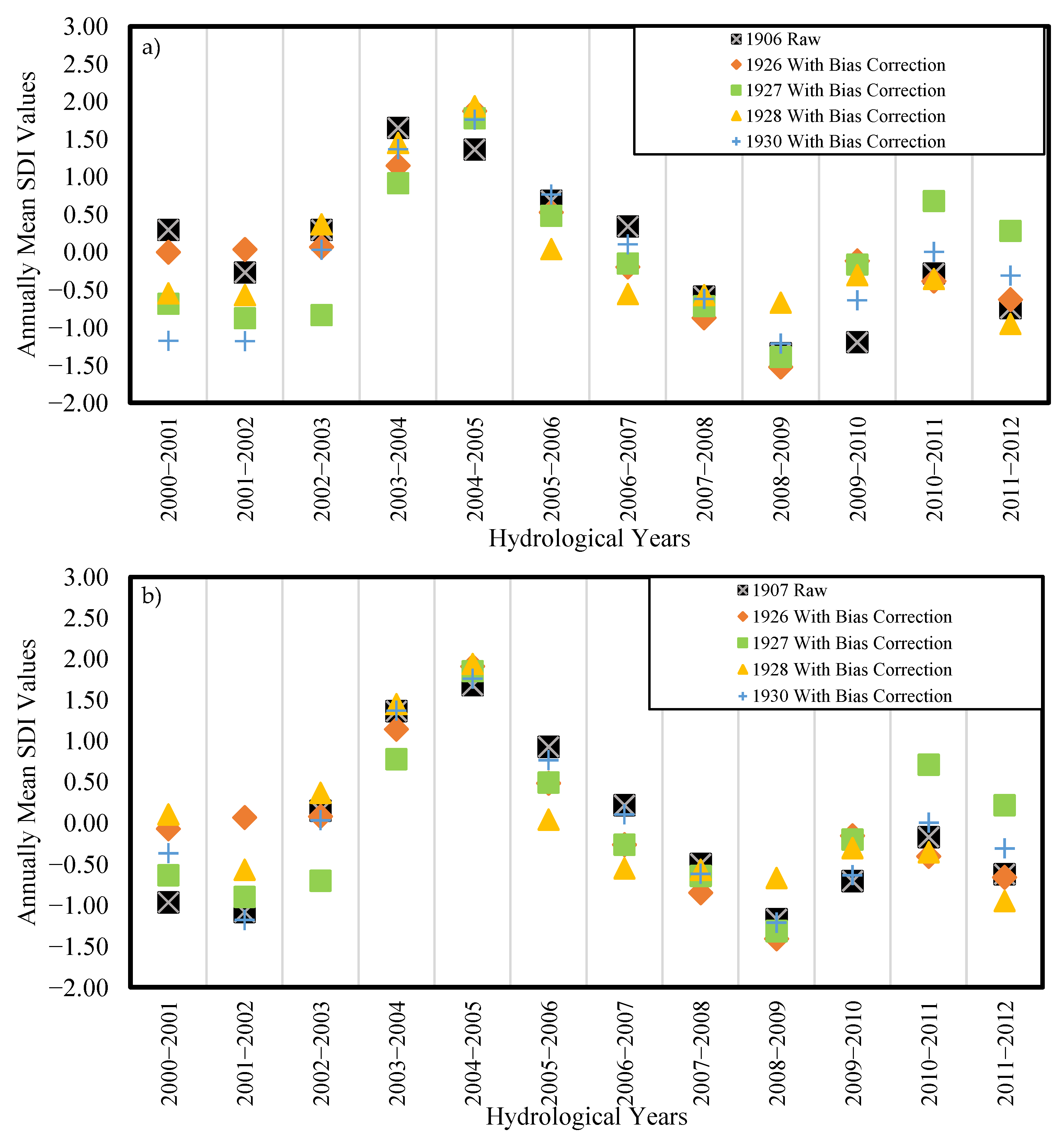
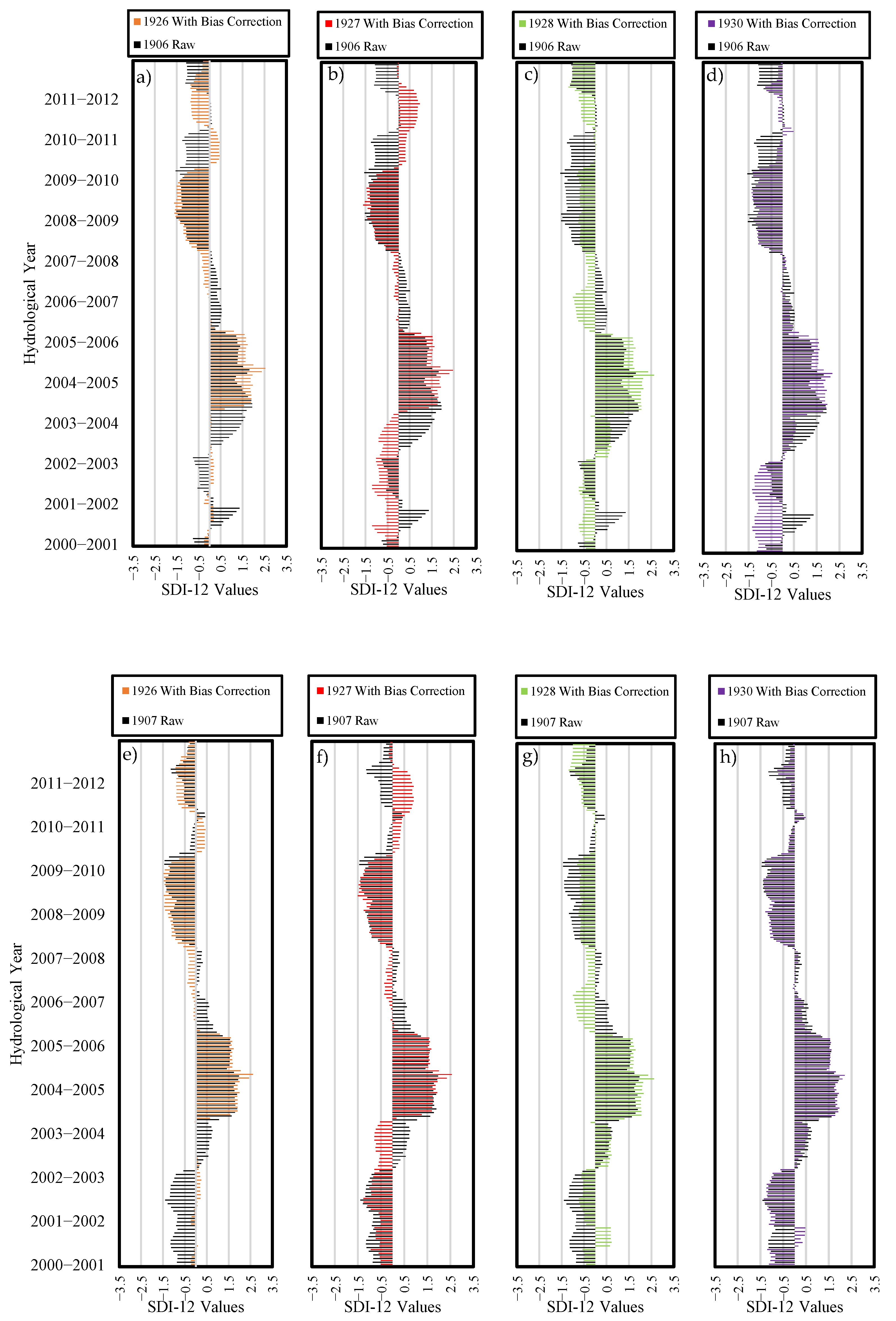
2.3. Streamflow Drought Index Method

The standardized precipitation index (SPI), which allows the numerical analysis of drought with indexes, has been used in the published literature [35,36,37]. The streamflow drought index (SDI) method is similar to the SPI calculation. This method was developed by Nalbantis and Tsakiris (2008) [38] in which only average flows are applied, rather than precipitation data, as the input. In cases where i represents any hydrological year, a month of this year is represented by j, the streamflow value by Qij, the cumulative flow volume by Vi,k, and Equation (9) is obtained as follows [24]:
V i , k = j = 1 3 k Q i , j     i = 1 , 2 , j = 1 , 2 , , 12 k = 1 , 2 , 3 , 4
where the k = 1 value represents the October to December period, k = 2 for October to March, k = 3 for October to June, and k = 4 for October to September. According to the volumes in Equation (9), for each k value of the hydrological year i, the SDI is obtained by Equation (10) [24]:
S D I i , k = V i , k V k ¯ σ k ,   k = 1 , 2 , 3 , 4          
In Equation (10), Vk and σk represent the mean and standard deviation of the cumulative volumes, respectively. Eight different classifications for the SDI method are examined. Table 2 shows these classifications in detail [23].

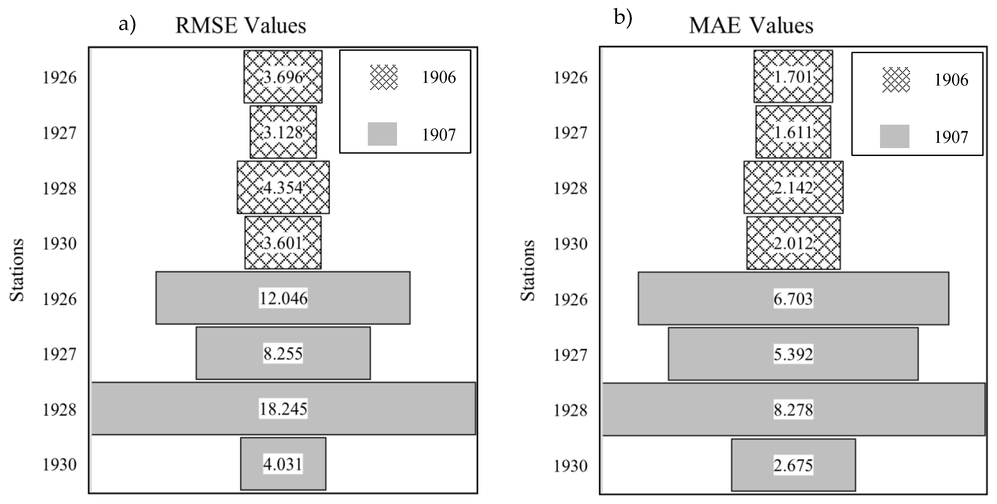
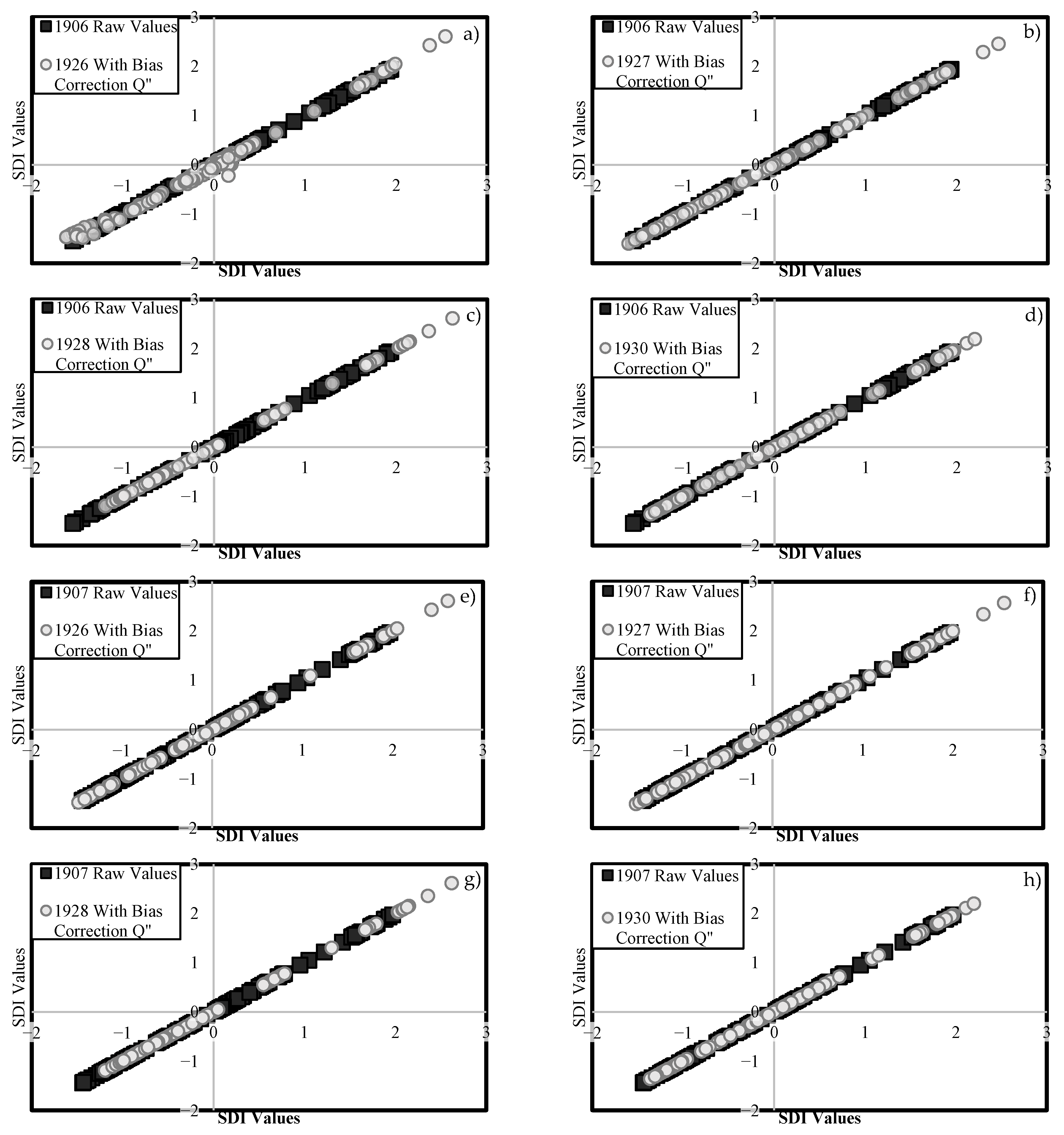
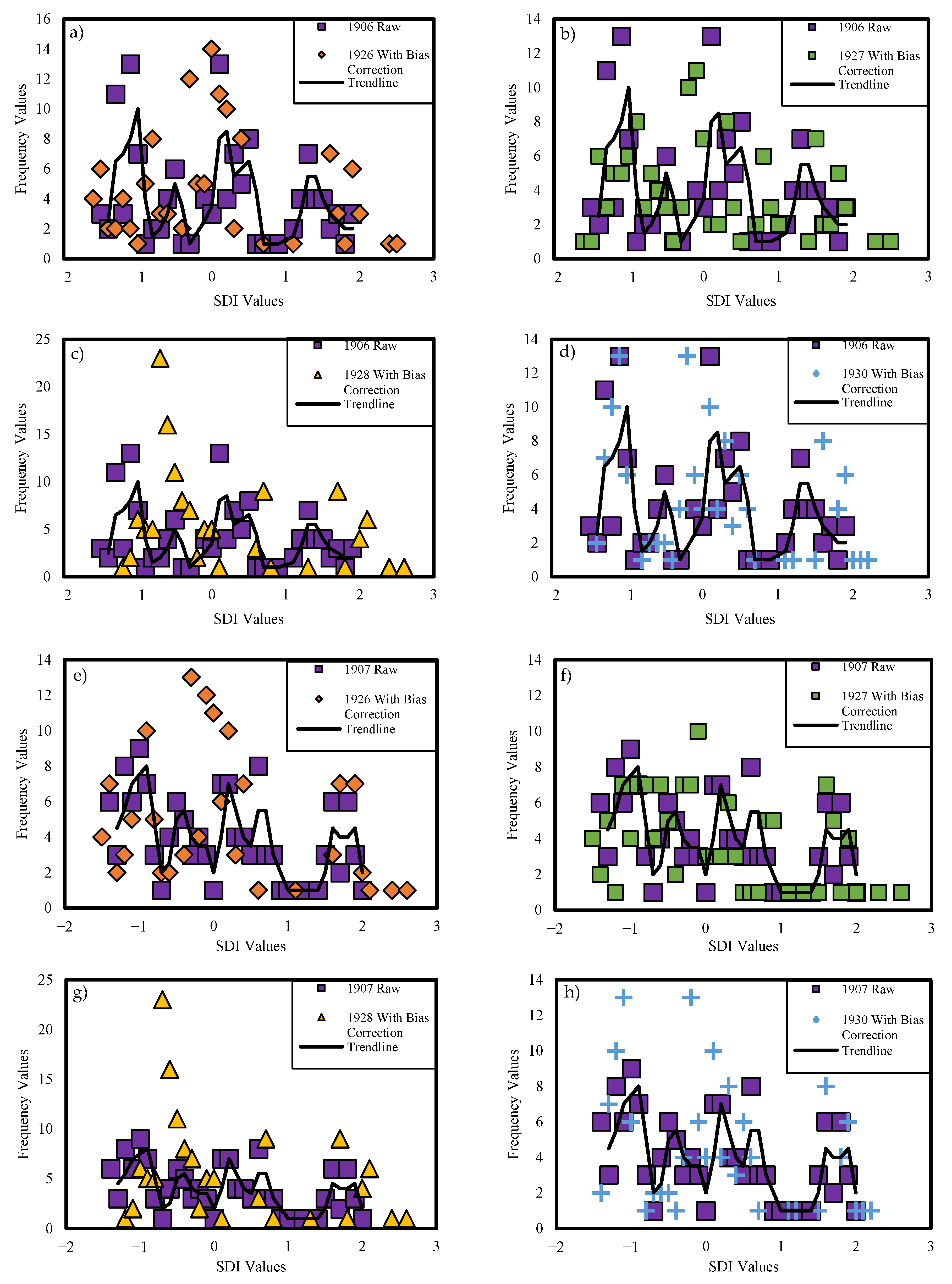
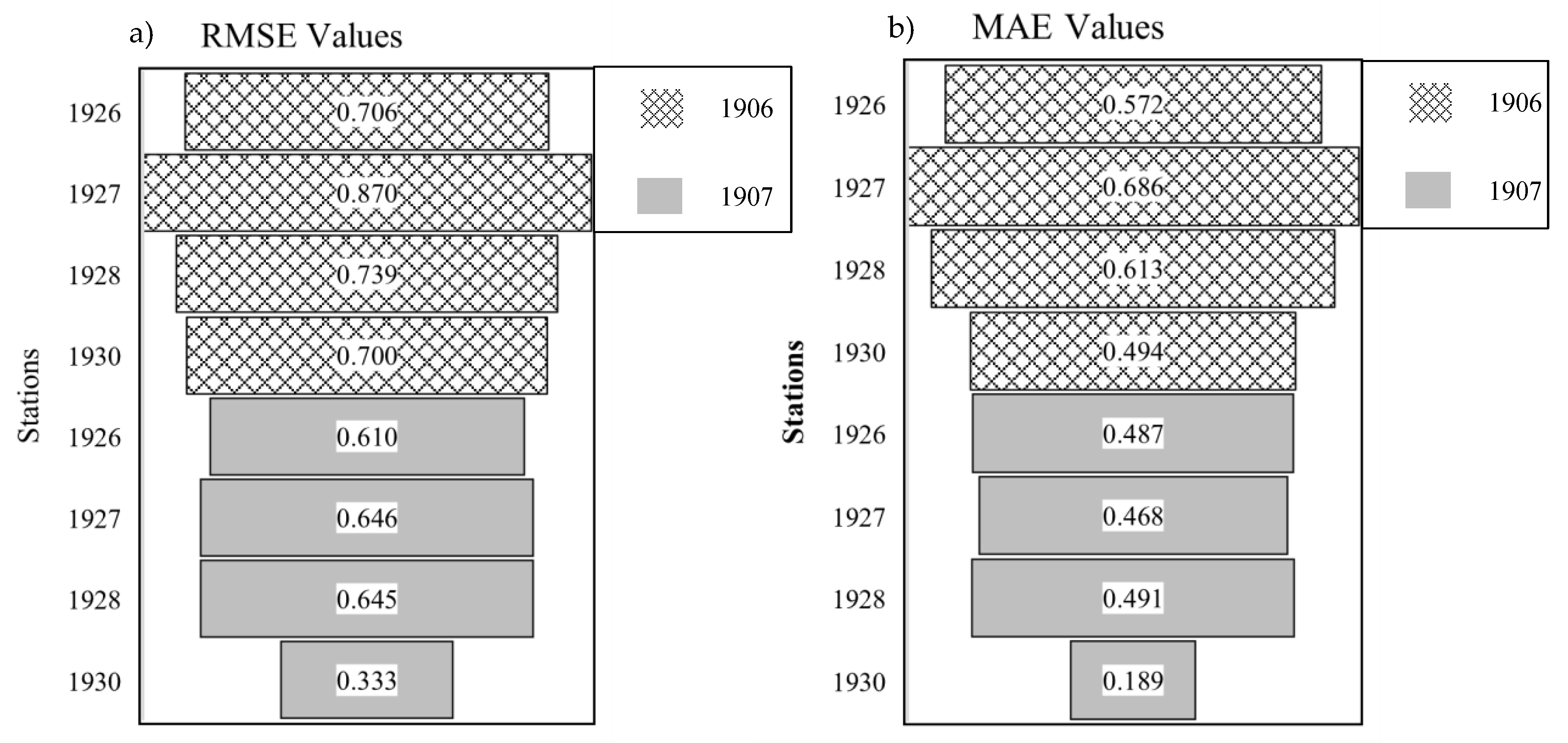
3. Results and Discussion

In this present study, to complete the missing data of stations 1906 and 1907, data from different observation stations, including D19A026, D19A027, D19A028 and D19A030, were transferred to the 1906 and 1907 SGSs in the same basin in proportion to their drainage areas. The recorded flow data at observation stations 1906 and 1907 were available until 2011. This study aimed to determine which interstation DAR method can be applied to complete the missing SGSs values for future probable hydrological works.
Examining the original data from the 1906 and 1907 stations, the maximum streamflow values were observed in 2005 (around the 50th month), and it was observed that there were decreases in the flow rates in the following years. The data were transferred to the target station points by applying directly and with bias correction. As seen in Figure 2 and Figure 3, the station data diverged significantly from the original values when they were moved directly in proportion to their areas.
However, as a result of the corrections made by using the ϕ and K values calculated with the statistical parameters from the observation stations, it was seen that the flow values converged significantly to the original values of the target stations. The obtained values as a consequence of the correction were re-evaluated to increase the convergence of the results. In the correction procedure, the transported values were not constant for the ϕ exponential and K coefficients, but the average flow values were obtained and included in the related equations [17].
Flow duration curves were created for a more detailed analysis of the convergence of the transported flow values with the target station values. Among the values transferred to the 1906 station, it was observed that only the D19A027 station provided a high level of approximation in terms of the probability of occurrence, while the other station values were realized at lower levels (Figure 3). In addition, it should be noted that the transfer process to the 1907 station had a satisfactory level of probability (Figure 4). Even if there were apparent deviations, a good fit was achieved. In general, it can be thought that the data transferred to the 1907 target station produced more consistent results. The conformity graphs between the bias-corrected data and the original data of the target stations are given in Figure 5.
These graphs show the deviation of the values carried by the linear trend line from the target values. As seen in Figure 5, the most consistent results with the method in this study were obtained by moving the station D19A030 to the target station 1907 SGS. This consistency was related to the proximity of the stations D19A030 and 1907 [11,14]. In addition, the data transferred to the 1906 station were clustered in the range from 0 to 10 m3/s, whereas the data transferred to 1907 were concentrated in the range from 0 to 40 m3/s. In general, in transporting lower data values, the conformity was higher. In other words, it was better represented. Larger values deviated more [14,16].
The root mean square error (RMSE) and MAE (mean absolute error) evaluation criteria were calculated to better understand the changes according to the linear trend lines of the data transferred to the target station (Figure 6).
The error rate increased considerably in the transfer cases where the drainage area ratios varied greatly, even if bias correction was applied (Figure 7). The SDI values calculated with the streamflow data transferred to the target stations are shown in Figure 8.
As far as the transfer of observed flow data in the published literature is concerned, no study has been found that looks at the effect it has on drought indexes. In studies conducted only on drought indexes, for example, Gümüş (2017) [21] stated that 2000 was a severely dry year for this region, while an extremely dry period was only mentioned in 2001 for a certain period.
In addition, Dikici (2020) [22] made similar inferences for drought situations between 2004 and 2005 in their study. With the transfer calculations in the present study, it was observed that the D19A026, D19A027 and D19A030 stations were estimated to be very close to the values obtained with the original data in terms of extreme dry periods. Still, there were some deviations in the prediction of mild dry periods.
It is noteworthy that the drought index results at the 1906 station between the 2003 and 2005 and between the 2007 and 2009 water years were quite compatible. In the 1907 station, the consistency of the SDI values obtained from the D19A030 SGS, was one of the first striking cases. The correlation coefficient (R) value of 0.97 supports this result. The SDI values obtained with the transported data of station D19A028 to the 1906 and 1907 SGSs had a low correlation in extremely dry periods. It is highly probable that D19A028 SGS, being far from the target stations, may have caused this result. The fact that the transferred flow rates represent similar ranges as the target station, the data can be considered an important comparison parameter; thus, the scatter plots of the SDI values are shown in a separate graph in Figure 9.
Considering the graphs in Figure 9, the fact that the D19A027 and D19A030 SGSs had similar scatter plots of SDI as the target station shows that the data were better represented. However, the SDI values at stations D19A026 and D19A028 were clustered in different regions according to the SDI indexes calculated with the original data of both the 1906 and 1907 SGSs. Although the original values were in the range from −2 to +2 SDI, all the transported stations were in the range from −2 to +3 SDI, indicating that the periods of extreme wet cannot be well determined. The annual average SDI values calculated over a 12 month time scale are given in Figure 10.
While the 2008 to 2009 water year stood out as the driest period for both of the target stations, it was seen that the SDI values were well estimated by stations D19A026, D19A027 and D19A030. The SDI values obtained with the data of station D19A028 transferred to the target station could not adequately predict the driest period. Examining the calculated SDI values and transfer results of the 1906 and 1907 stations with the original data, the wet periods seen in the 2004 to 2005 water years were well represented by all stations. The original values of the target stations and the frequency graphs of the SDI values created with the transferred data are shown in Figure 11. It is possible to point out the mild drought period as the most striking period in all the graphs.
It can be seen in these graphs that the results of the D19A028 station and the target station values showed little convergence. In addition, according to the trend line created for the original SDI frequency values, no more than two indexes were found, while it is possible to see larger values in the transported SDI values. This can be expressed as dry periods producing more consistent results than wet periods. The graphs in Figure 12 were created to compare the original and bias-corrected SDI values. In these graphs, it is seen that SDI data are clustered during the dry period. The clustering of the SDI values on the trendline indicates that the values moved by bias correction converge to the target station values, which can be seen mostly in the drought periods. In addition, the deviation of the values from the trendline, shows itself as a scattering point, meaning that despite the bias correction there are some values for which an adequate approach cannot be achieved (Figure 12).
It was determined that this situation occurred in direct proportion to the R values, and, accordingly, as a result of the DAR method, the most suitable station match for moving to the nearest station was 1930–1907, and the least compatible match was 1927–1907. The results of RMSE and MAE evaluation criteria in terms of the SDI analysis in the DAR method are given in Figure 13. As seen from this figure, the fact that the selected stations were closer to the target station D19A07 ensured that the error rate in the index values was less. While the highest error values were determined at station D19A027, the least error was obtained with data from station D19A030. Determining the mean flow values of the ϕ and K coefficients because of bias correction significantly reduced these deviations [16,17].
Contour mappings were created between the target station SDI and the index values generated by the flow rates (Figure 14).
Examining these graphs shows good consistency, especially in the values representing the dry periods. The correlation between the data in terms of the wet periods was lower. It is mentioned that the normal ratio method can be evaluated in addition to the arithmetic average, inverse distance technique, coefficient of correlation techniques and artificial intelligence applications in terms of completing the missing flow data in many studies in the literature [10,38]. Similar to the normal ratio method, within the scope of this study, the applicability of the DAR method was evaluated. In addition to the streamflow drought index, there are different drought indices in the literature, such as the standardized runoff index (SRI), standardized streamflow index (SSI) and low flow index (LFI), in which streamflow data are used. Although statistical distributions usually change within these calculations, there may also be cases where low flows are evaluated [39,40,41]. In the following years, studies using these drought index can be performed.

4. Conclusions

In this study, the data from six different streamflow gauge stations (SGSs) located in the Asi River sub-basin, where there are fertile plains and intense agricultural activities in Turkey, were used to transfer the data to other observation stations. The average monthly data from the selected stations between the years 2000 and 2011 were used. The obtained results were compared with the original data of the transferred stations, and the ability of the method to converge to the existing data was investigated. In addition, bias correction was applied to these data, and the effect on the transferred data was examined. Although there are many studies in the literature that used the DAR and SDI methods, there are no studies evaluating both methods together. Therefore, it is thought that the obtained results in this study will make positive contributions to the published literature. In recent years, studies of the region’s meteorological and agricultural drought effects have been notable. Therefore, in terms of the analysis of the accuracy of the method, the streamflow drought index’s (SDI) application—one of the hydrological indexes—was performed over a 12 month timescale.
Considering the data transferred directly to the target stations in proportion to their area because of this study, a significant divergence from the original values stands out. However, it is striking that the flow rates converged to the target station data when correction was applied. The proximity of the existing stations to each other produced very highly correlated results, both in the direct transfer process and when the correction was applied. Similarly, in terms of the drought index calculations, correlation values close to 97% were seen in the original and transferred flow rates. It can be stated that dry periods produced more consistent results than humid periods. When the evaluation criteria, namely, RMSE and MAE, were examined, the obtained error rates were quite similar to the results for the dry and wet periods. Moreover, time-varying contour mappings were created for the target station values where the highest agreement was observed. It is possible to say that there was a good consistency in the values representing the dry periods on the maps, whereas the correlation was lower in the wet periods. In considering the effective management stages of the water resources, it can be predicted that the transportation of the basin-based observation station data, by making corrections according to the drainage areas, will have positive contributions, especially in the design of hydraulic structures and cost calculations. It is thought that the practical application of these methods will have a favorable impact on decision-making processes for drought and flow hydrological studies. In the following years, many studies can be carried out in which various hydrometeorological variables of water collection basins and new transfer methods will be researched with an integrated approach. In particular, different streamflow transfer and drought index methods can be focused on issues, such as low flows threshold value, volume, length, and duration period.

Author Contributions

Conceptualization, E.T. and S.D.Ş.; methodology, E.T. and S.D.Ş.; software, S.D.Ş.; formal analysis, E.T. and S.D.Ş.; investigation, E.T. and S.D.Ş.; writing—original draft preparation, E.T. and S.D.Ş.; writing—review and editing, E.T. and S.D.Ş.; visualization, E.T. and S.D.Ş.; supervision, E.T. All authors have read and agreed to the published version of the manuscript.

Funding

This research received no external funding.

Institutional Review Board Statement

Not applicable.

Informed Consent Statement

Not applicable.

Data Availability Statement

Not applicable.

Acknowledgments

The authors wish to thank the General Directorate of State Hydraulic Works (known as DSI, Location: Ankara, Turkey) for sharing the streamflow gauge station data used in this study. Furthermore, we are grateful for the valuable support provided by Ömer Faruk ÇAPAR in carrying out this research.

Conflicts of Interest

The authors declare no conflict of interest.

References

  1. Akçakoca, F.; Apaydın, H. Modelling of Bektas Creek daily streamflow with Generalized Regression Neural Network Method. Int. J. Adv. Sci. Res. Eng. 2020, 6, 97–103. [Google Scholar] [CrossRef]
  2. Mesta, B.; Akgun, O.B.; Kentel, E. Alternative solutions for long missing streamflow data for sustainable water resources management. Int. J. Water Resour. Dev. 2021, 37, 882–905. [Google Scholar] [CrossRef]
  3. Asaad, M.N.; Eryürük, Ş.; Eryürük, K. Forecasting of streamflow and comparison of artificial intelligence methods: A case study for Meram Stream in Konya, Turkey. Sustainability 2022, 14, 6319. [Google Scholar] [CrossRef]
  4. Turhan, E.; Özmen-Çağatay, H. Using of Artificial Neural Network (ANN) for setting estimation model of missing flow data: Asi River-Demirköprü Flow Observation Station (FOS). Çukurova Üniversitesi Mühendislik Mimar. Fakültesi Derg. 2016, 31, 93–106. [Google Scholar] [CrossRef] [Green Version]
  5. Loganathan, P.; Mahindrakar, A.B. Intercomparing the robustness of machine learning models in simulation and forecasting of streamflow. J. Water Clim. Chang. 2021, 12, 1824–1837. [Google Scholar] [CrossRef]
  6. Kilinc, H.C. Daily streamflow forecasting based on the hybrid Particle Swarm Optimization and Long Short-Term Memory model in the Orontes Basin. Water 2022, 14, 490. [Google Scholar] [CrossRef]
  7. Üneş, F.; Demirci, M.; Zelenakova, M.; Çalışıcı, M.; Taşar, B.; Vranay, F.; Kaya, Y.Z. River Flow Estimation Using Artificial Intelligence and Fuzzy Techniques. Water 2020, 12, 2427. [Google Scholar] [CrossRef]
  8. Yilmaz, M.; Tosunoğlu, F.; Kaplan, N.H.; Üneş, F.; Hanay, Y.S. Predicting monthly streamflow using artificial neural networks and wavelet neural networks models. Model. Earth Syst. Environ. 2022, 8, 5547–5563. [Google Scholar] [CrossRef]
  9. Mehraein, M.; Mohanavelu, A.; Naganna, S.R.; Kulls, C.; Kisi, O. Monthly Streamflow Prediction by Metaheuristic Regression Approaches Considering Satellite Precipitation Data. Water 2022, 14, 3636. [Google Scholar] [CrossRef]
  10. Hamzah, F.B.; Hamzah, F.M.; Razali, S.F.M.; Jaafar, O.; Jamil, N.A. Imputation methods for recovering streamflowobservation: A methodological review. Cogent Environ. Sci. 2020, 6, 1745133. [Google Scholar] [CrossRef]
  11. Ergen, K.; Kentel, E. An integrated map correlation method and multiple-source sites drainage-area ratio method for estimating streamflows at ungauged catchments: A case study of Western Black Sea Region, Turkey. J. Environ. Manag. 2016, 166, 309–320. [Google Scholar] [CrossRef] [PubMed]
  12. Li, Q.; Peng, Y.; Wang, G.; Wang, H.; Xue, B.; Hu, X. A Combined Method for Estimating Continuous Runoff by Parameter Transfer and Drainage Area Ratio Method in Ungauged Catchments. Water 2019, 11, 1104. [Google Scholar] [CrossRef] [Green Version]
  13. Saka, F.; Babacan, H.T. Discharge Estimation by Drainage Area Ratio Method at Some Specific Discharges for 2251 Stream Gauging Station in East Black Sea Basin, Turkey. J. Investig. Eng. Technol. 2019, 2, 309–320. [Google Scholar]
  14. Yılmaz, M.U.; Önöz, B. Evaluation of statistical methods for estimating missing daily streamflow data. Tek. Dergi 2019, 30, 9597–9620. [Google Scholar] [CrossRef] [Green Version]
  15. Yılmaz, M.U.; Önöz, B. A comparative study of statistical methods for daily streamflow estimation at ungauged basins in Turkey. Water 2020, 12, 459. [Google Scholar] [CrossRef] [Green Version]
  16. Bakış, R.; Şirin, F.Ç.; Bayazıt, Y. Linear Analysis of Region-Ratio Method for Flow Gauges. İklim Değişikliği Ve Çevre Derg. 2020, 5, 8–15. [Google Scholar]
  17. Değerli, S.; Turhan, E. Investigation of Streamflow Data Accuracy with Bias Correction Using Drainage Area-Ratio Method. Eur. J. Sci. Technol. 2022, 34, 100–104. [Google Scholar] [CrossRef]
  18. Turhan, E.; Değerli, S. A Comparative Study of Probability Distribution Models for Flood Discharge Estimation: Case of Kravga Bridge, Turkey. Cas. Geofiz. J. 2022, 39, 243–257. [Google Scholar] [CrossRef]
  19. Turhan, E. An Investigation on the Effect of Outliers for Flood Frequency Analysis: The Case of the Eastern Mediterranean Basin, Turkey. Sustainability 2022, 14, 16558. [Google Scholar] [CrossRef]
  20. Djamel, B.; Houari, Z.; Fares, B. Floods and Hydrograms of Floods of Rivers in Arid Zones of the Mediterranean, Case of the Kingdom of Morocco. Int. J. Geosci. 2020, 11, 651–666. [Google Scholar] [CrossRef]
  21. Gümüş, V. Hydrological drought analysis of Asi River Basin with Streamflow Drought Index. GU J. Sci. Part C 2017, 5, 65–73. [Google Scholar]
  22. Dikici, M. Drought analysis with different indices for the Asi Basin (Turkey). Sci. Rep. 2020, 10, 20739. [Google Scholar] [CrossRef] [PubMed]
  23. Turhan, E.; Çulha, B.D.; Değerli, S. Hydrological evaluation of Streamflow Drought Index method for different time scales: A case study of Arsuz Plain, Turkey. J. Nat. Hazards Environ. 2022, 8, 25–36. [Google Scholar] [CrossRef]
  24. Turhan, E.; Değerli, S.; Çatal, E.N. Long-term hydrological drought analysis in agricultural irrigation area: The case of Dörtyol-Erzin Plain, Turkey. Curr. Trends Nat. Sci. 2022, 21, 501–512. [Google Scholar] [CrossRef]
  25. Topçu, E.; Seçkin, N.; Haktanır, N.E. Drought analyses of Eastern Mediterranean, Seyhan, Ceyhan, and Asi Basins by using aggregate drought index (ADI). Theor. Appl. Climatol. 2022, 147, 909–924. [Google Scholar] [CrossRef]
  26. Nalbantis, I.; Tsakiris, G. Evaluation of a Hydrological Drought Index. Eur. Water 2008, 23, 67–77. [Google Scholar] [CrossRef]
  27. Abbas, A.; Waseem, M.; Ullah, W.; Zhao, C.; Zhu, J. Spatiotemporal analysis of meteorological and hydrological droughts and their propagations. Water 2021, 13, 2237. [Google Scholar] [CrossRef]
  28. Kubiak-Wójcicka, K.; Nagy, P.; Zelenáková, M.; Hlavatá, H.; Abd-Elhamid, H.F. Identification of Extreme Weather Events Using Meteorological and Hydrological Indicators in the Laborec River Catchment, Slovakia. Water 2021, 13, 1413. [Google Scholar] [CrossRef]
  29. Katipoğlu, O.M.; Acar, R.; Şenocak, S. Spatio-temporal analysis of meteorological and hydrological droughts in the Euphrates Basin, Turkey. Water Supply 2021, 21, 1657–1673. [Google Scholar] [CrossRef]
  30. Zhang, Q.; Miao, C.; Gou, J.; Wu, J.; Jiao, W.; Song, Y.; Xu, D. Spatiotemporal characteristics of meteorological to hydrological drought propagation under natural conditions in China. Weather. Clim. Extrem. 2022, 38, 100505. [Google Scholar] [CrossRef]
  31. The State Hydraulic Works (knownly as DSI). Annual Streamflow Observation Records (1986–2020). Head of Study and Planning Department, Ankara. 2015. Available online: https://www.dsi.gov.tr/Sayfa/Detay/744 (accessed on 15 September 2022).
  32. Nalcıoğlu, A.; Ünsal, M.; Ercan, B.; Yağcı, A.E. Modeling of hydrometeorological factors with discharge in Asi Basin. KSU J. Agric. Nat. 2020, 23, 1510–1517. [Google Scholar] [CrossRef]
  33. Geçen, R.; Usun, Ç.F. Orontes River, it’s basin, international usage and problems. Elazığ, Türkiye. Int. Symp. Geomorphol. 2017, 636–644. Available online: http://www.ujes.org/anasayfa/ (accessed on 15 September 2022).
  34. Emerson, D.G.; Vecchia, A.V.; Dahl, A.L.; United States Geological Survey (USGS); Bureau of Reclamation. Evaluation of Drainage-Area Ratio Method Used to Estimate Streamflow for the Red River of the North Basin, North Dakota and Minnesota; US Department of the Interior: Washington, DC, USA; US Geological Survey: Reston, VA, USA, 2005.
  35. Fung, K.F.; Huang, Y.F.; Koo, C.H.; Tan, K.W. Standardized Precipation Index (SPI) and Standardized Precipation Evapotranspiration Index (SPEI) drought characteristic and trend analysis using the second generation canadian earth system model (CanESM2) outputs under representative concentration pathway (RCP) 8.5. Carpathian J. Earth Environ. Sci. 2019, 14, 399–408. [Google Scholar] [CrossRef]
  36. Safarianzengir, V.; Sobhani, B. Simulation and analysis of natural hazard phenomenon, drought in Southwest of The Caspian Sea, Iran. Carpathian J. Earth Environ. Sci. 2020, 15, 127–136. [Google Scholar] [CrossRef]
  37. Moccia, B.; Mineo, C.; Ridolfi, E.; Russo, F.; Napolitano, F. SPI-Based Drought Classification in Italy: Influence of Different Probability Distribution Functions. Water 2022, 14, 3668. [Google Scholar] [CrossRef]
  38. Norliyana, W.; Ismail, W.; Zawiah, W.; Zin, W.; Ibrahim, W. Estimation of rainfall and streamflow missing data for Terengganu, Malaysia by using interpolation technique methods. Malays. J. Fundam. Appl. Sci. 2017, 13, 213–217. [Google Scholar] [CrossRef]
  39. Turhan, E.; Kaya Keleş, M.; Tantekin, A.; Keleş, A.E. The Investigation of the Applicability of Data-Driven Techniques in Hydrological Modeling: The Case of Seyhan Basin. Rocz. Ochr. Sr. 2019, 21, 29–51. [Google Scholar]
  40. Salimi, H.; Asadi, E.; Darbandi, S. Meteorological and Hydrological Drought Monitoring Using Several Drought Indices. Appl. Water Sci. 2021, 11, 11. [Google Scholar] [CrossRef]
  41. Cammalleri, C.; Vogt, J.; Salamon, P. Development of an operational low-flow index for hydrological drought monitoring over Europe. Hydrol. Sci. J. 2017, 62, 346–358. [Google Scholar] [CrossRef]
Figure 2. Temporal changes in the streamflow values for the number 1906 SGS. (a) 1926 to 1906, (b)1927 to 1906, (c) 1928 to 1906, (d) 1930 to 1906.
Water 15 00425 g002
Figure 3. Temporal changes in the streamflow values for the number 1907 SGS. (a) 1926 to 1907, (b)1927 to 1907, (c) 1928 to 1907, (d) 1930 to 1907.
Water 15 00425 g003
Figure 4. Flow duration curves for the number 1906 SGS. (a) 1926 to 1906, (b)1927 to 1906, (c) 1928 to 1906, (d) 1930 to 1906.
Water 15 00425 g004
Figure 5. Flow duration curve for the number 1907 SGS. (a) 1926 to 1907, (b)1927 to 1907, (c) 1928 to 1907, (d) 1930 to 1907.
Water 15 00425 g005
Figure 6. Correlation plot between the original and bias-corrected values for the number 1906 and 1907 SGSs. (a) 1926 to 1906, (b) 1927 to 1906, (c) 1928 to 1906, (d) 1930 to 1906, (e) 1926 to 1907, (f)1927 to 1907, (g) 1928 to 1907, (h) 1930 to 1907. Linear regression line represented with grey, x=y graph represented with black colored line.
Water 15 00425 g006aWater 15 00425 g006b
Figure 7. RMSE and MAE values in the transfer cases for applying bias correction. (a) RMSE results, (b) MAE results.
Water 15 00425 g007
Figure 8. Obtained SDI-12 values for the transfer cases to the target SGSs. (a) 1926 and 1906, (b) 1927 and 1906, (c) 1928 and 1906, (d) 1930 and 1906, (e) 1926 and 1907, (f) 1927 and 1907, (g) 1928 and 1907, (h) 1930 and 1907.
Water 15 00425 g008
Figure 9. Scatter plots of SDI-12 values. (a) 1926 and 1906, (b) 1927 and 1906, (c) 1928 and 1906, (d) 1930 and 1906, (e) 1926 and 1907, (f) 1927 and 1907, (g) 1928 and 1907, (h) 1930 and 1907.
Water 15 00425 g009
Figure 10. The mean annual SDI values for the raw (original) data and the other station data with bias correction. (a) 1906 comparisons, (b) 1907 comparisons.
Water 15 00425 g010
Figure 11. Frequency values for the raw (original) and transferred to the other station data with bias correction. (a) 1926 and 1906, (b) 1927 and 1906, (c) 1928 and 1906, (d) 1930 and 1906, (e) 1926 and 1907, (f) 1927 and 1907, (g) 1928 and 1907, (h) 1930 and 1907.
Water 15 00425 g011
Figure 12. Raw and bias-corrected SDI values comparison. (a) 1926 and 1906, (b) 1927 and 1906, (c) 1928 and 1906, (d) 1930 and 1906, (e) 1926 and 1907, (f)1927 and 1907, (g) 1928 and 1907, (h) 1930 and 1907. Linear regression line represented with yellow line.
Water 15 00425 g012aWater 15 00425 g012b
Figure 13. RMSE and MAE values for the SDI results. (a) RMSE results, (b) MAE results.
Water 15 00425 g013
Figure 14. Contour maps for the 1907 SGS raw data, the SDI results with the original values and the SDI values with the transferred flow data. (a) 1907 and 1930 3D Mesh graph over time, (b) 1907 and 1930 contour graph over time.
Water 15 00425 g014
Table 1. SGSs general information [33].
Station No.Latitude (N)Longitude (E)Drainage Area (km2)
D19A026 (1926)36°57′03″33°02′11″2689.2
D19A027 (1927)36°39′34″34°00′02″1005.2
D19A028 (1928)36°10′32″32°23′44″313.2
D19A030 (1930)36°10′32″32°23′44″313.2
190636°10′32″32°23′44″313.2
190736°10′32″32°23′44″313.2
Table 2. Drought classification [23].
Index ValueCategory
SDI ≤ −2Extreme drought
−2 < SDI ≤ −1.5Severe drought
−1.5 < SDI ≤ −1Moderate drought
−1 < SDI ≤ 0Mild drought
0 < SDI ≤ 1Mildly wet
1 < SDI ≤ 1.5Moderately wet
1.5 < SDI ≤ 2Severely wet
SDI > 2Extremely wet
Disclaimer/Publisher’s Note: The statements, opinions and data contained in all publications are solely those of the individual author(s) and contributor(s) and not of MDPI and/or the editor(s). MDPI and/or the editor(s) disclaim responsibility for any injury to people or property resulting from any ideas, methods, instructions or products referred to in the content.

