An Improved DINEOF Algorithm Based on Optimized Validation Points Selection Method

Abstract

Ocean remote-sensing satellite data have been widely applied in the areas of oceanography, meteorology, the environment, and many more fields in science and engineering. However, missing data due to cloud cover, equipment failure, etc., limit its application. Therefore, reconstruction of the missing data through an appropriate method is essential. The data-interpolating empirical orthogonal function (DINEOF) algorithm proposed by Beckers and Rixen (2003) is currently the most commonly used method for the reconstruction of missing data in large areas. However, the existing DINEOF algorithm adopts a random method to select the cross−validation points, which may underutilize effective information around the missing value points. In addition, the cross-validation points may be too concentrated in an area, thus being unable to reflect the overall characteristics of the data. This paper optimizes the method to select the cross-validation points so that the information around the missing values can be effectively utilized and to avoid the cross-validation points being too concentrated. On this basis, an improved validation-point DINEOF algorithm (IV−DINEOF) is proposed. An ideal dataset and a reanalysis dataset based on sea surface temperature (SST) are used to test the performance of the improved algorithm. Statistical analysis of the results shows that the data reconstruction performance of the IV−DINEOF algorithm is better than that of the DINEOF algorithm, and the computational efficiency is also improved. The VE−DINEOF algorithm has the highest computing efficiency, but its reconstruction accuracy is lower than that of IV−DINEOF.

1. Introduction

Marine satellites can achieve large-scale and long-term observations of the oceans and provide data sources for understanding the oceans that cannot be replaced by other observation methods [1]. The complete marine satellite remote-sensing data are important for research concerning the carbon cycle in the ocean–atmosphere system, red tide monitoring, environmental assessment, fishery management, etc. [2]. However, data may be partially or widely missing due to cloud cover, satellite malfunction, image noise, etc. Missing data will seriously affect the utilization of the acquired data [3]. Thus, it is particularly important to use reliable methods to reconstruct the missing data.

To obtain complete satellite remote-sensing data, a variety of data reconstruction and processing methods have been developed, such as optimal interpolation (OI) [4,5], empirical orthogonal function decomposition (EOF) [6], expectation maximization method (EM) [7], singular spectrum method (SSA) [8,9], Kalman filter (KF) [10], and variational data assimilation (VDA) [11]. Moctar Dembélé et al. (2019) used the direct sampling (DS) algorithm to fill in missing data in the daily flow records of the Volta River basin in West Africa [12]. Fu et al. (2020) used a machine learning (ML) model called long short-term memory (LSTM) to predict the flow of the Kelantan River in the northeastern region of Peninsular Malaysia and compared the model with a classical backpropagation neural network model [13]. Fabio Oriani et al. (2020) used seven algorithms, including the vector sampling (VS) algorithm, to estimate missing rainfall data from five regions, including Denmark, Australia, and Switzerland [14]. Most of these methods are limited by the original condition of the data or rely on information such as related parameters and prior values, and they have limitations in the application and computational efficiency [15]. For machine learning methods, if there are not enough complete datasets to train the model, it is not possible to accurately reconstruct or predict the missing data [16]. However, it is usually difficult to obtain a complete data set. The DINEOF (Data Interpolating Empirical Orthogonal Functions) method proposed by Beckers and Rixen (2003) has advantages that other reconstruction methods do not have, such as no prior value, self-adaptation, and spatio-temporal correlation, and it is suitable for large-area missing data reconstruction. It has been widely used recently in the fields of oceanography, meteorology, the environment, and image processing [15].

The original DINEOF algorithm requires a random selection of data (i.e., usually 3%) as the cross-validation points while constructing the space-time matrix. However, the number and distribution of the cross-validation points may affect the accuracy of the interpolation. Ping et al. [3] proposed an improved DINEOF algorithm (I−DINEOF) based on DINEOF in 2015. Different from the DINEOF algorithm, which uses a single EOF to reconstruct the entire data matrix, the I−DINEOF algorithm divides the original matrix into multiple sub-regions and uses the optimal EOF suitable for each different sub-regions. Ping et al. [17] proposed an improved algorithm VE−DINEOF based on the DINEOF algorithm in 2016. In this algorithm, the optimal EOFs are variable. The algorithm uses the EOF that is most suitable for each iteration during reconstruction. In 2021, Zhang et al. [18] proposed the same distance stratification DINEOF (SDS−DINEOF) algorithm, which divides the Bohai Sea into 32 layers at equal distances according to their distance from the coast and uses each layer to mask the original dataset of the DINEOF method. DINEOF reconstruction is performed on the sub-datasets separately, and the results are combined into the final reconstructed dataset [18].

However, the problem with the I−DINEOF algorithm proposed by Ping (2015) is that the most suitable sub-region size is difficult to determine, and the calculation time increases simultaneously [3]. Beckers’ (2003) DINEOF algorithm, Ping’s (2016) VE−DINEOF algorithm, and Zhang’s (2021) SDS−DINEOF algorithm adopt a random method to select the cross-validation points, which could not effectively reflect the characteristics in the neighborhood of the missing values, or the cross-validation points may be too concentrated in several areas, thus not reflecting the overall characteristics of the dataset [6,17,18].

In response to the above problems, this paper proposes an optimized method to select the cross-validation points. On the basis of this, the DINEOF algorithm proposed by Beckers in 2003 is improved, and the IV−DINEOF (Improved Validation-point DINEOF) algorithm is proposed. The performance of the IV−DINEOF algorithm is tested using an ideal dataset and a constructed dataset based on the sea surface temperature (SST) reanalysis data. Since the IV−DINEOF method is able to choose lower optimal EOFs, the error information brought on by the introduction of higher-order modes is decreased. As a result, the revised algorithm can produce superior reconstruction results to the DINEOF approach.

2. The Improved Validation-Point DINEOF Algorithm

DINEOF algorithm uses randomly selected cross-validation points that cannot effectively reflect the characteristics in the neighborhood of the missing values. To solve this problem, this study improved the selection method of the cross-validation points. The improved algorithm preferentially selects the effective value points for cross-validation close to the missing points. Beckers (2006) also proposed a similar idea [19]. However, this study recommended the idea only as a guess in another method and did not fully elaborate on the idea, providing no testing. The improved algorithm and the reconstruction process involve the following six steps:

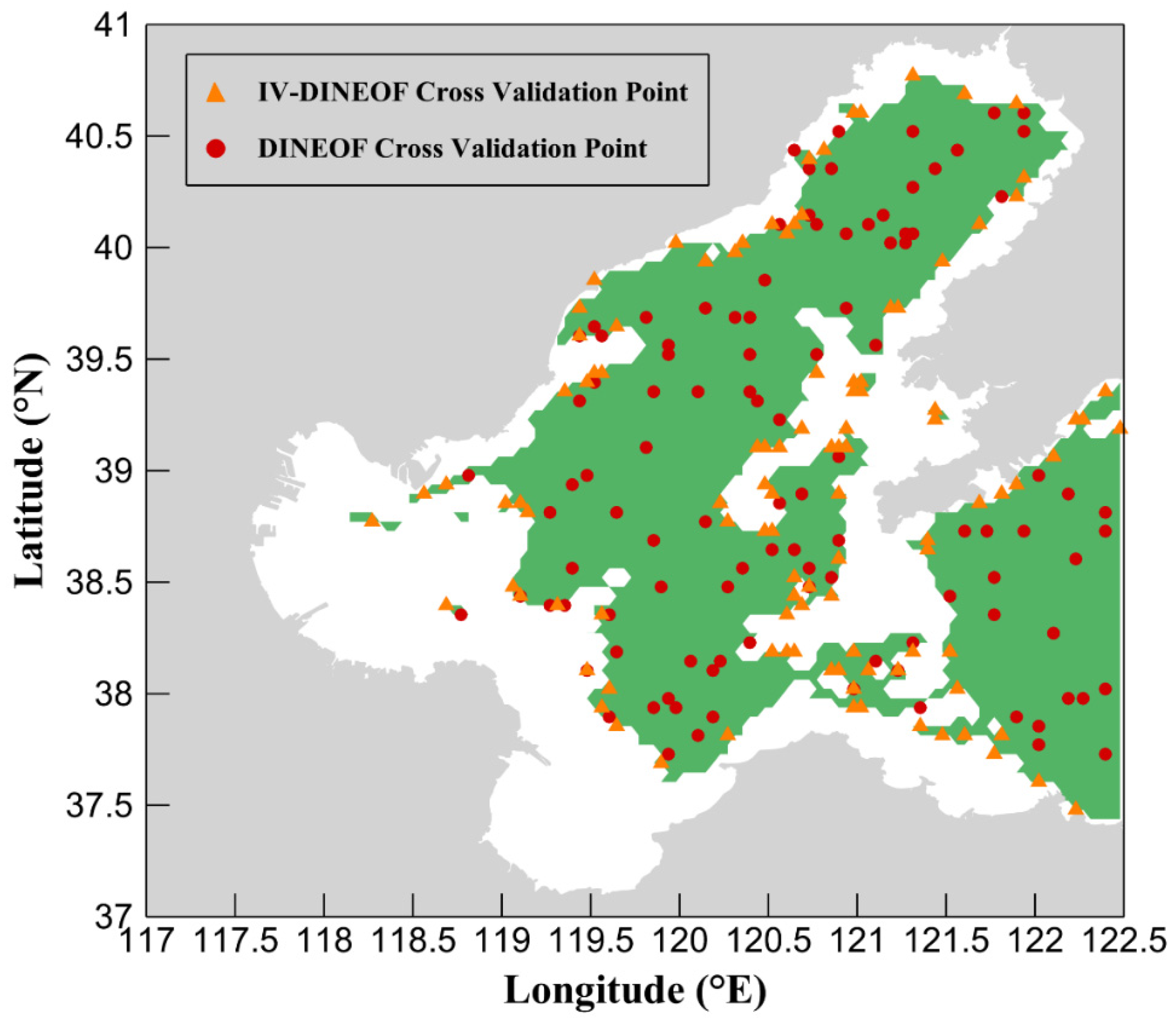
(1) Fill the original dataset, including missing data points, into the initial matrix X of $M\times N$, where M is the number of pixels in a single image, and N is the total number of images ($M\times N$ for Dataset1 is 201 × 121, and for Dataset2 is 5747 × 218). The valid data points are subtracted from the mean, and the missing data points are set to 0 (considered as an unbiased estimate). At the same time, 3% of the total valid data points are randomly selected as cross-validation points, and their value is set to 0. The improvement of this algorithm is that the cross-validation points are selected from valid data points that are in the neighborhoods of the missing data, as shown in Figure 1.

(2) Perform SVD decomposition on X ($X=U\times S\times V^T$), where U is the spatial mode of X, and the dimension is $M\times M$; S is the singular value of X, the dimension is $M\times N$, the values on the main diagonal run from large to small, and the values outside the main diagonal are 0; V is the time mode of X, and the dimension is $N\times N$.

(3) Reconstruct the missing values using the following formula:

$$\begin{array}{c}{X}_r={\displaystyle {\displaystyle \sum }_{p=1}^k}{\sigma }_P{u}_p{v}_P^T\end{array}$$

(1)

where k is the maximal number of EOFs. $u_p$ is the p-th spatial mode of X, that is, the p-th column of U. $v_p$ is the p-th time mode of X, that is, the p-th column of V. ${\sigma }_P$ is the p-th singular value of X. Return the corresponding missing value data in $X_r$ back to X after reconstruction.

(4) Repeat Steps (2) and (3) until the root mean square errors of the cross-validation points between the two iteration steps is less than the pre-set threshold ($e={10}^{-6}$). To prevent falling into an infinite loop, the maximum number of the iteration is set to 100. Calculate and store the root mean square error (RMSE) between the reconstructed values after convergence with the original value.

(5) Let $k=2,3,4,5,\dots ,r$ and repeat Steps (2), (3), and (4).

(6) Select k, the optimal number of EOFs corresponding to the minimum root mean square error, then reconstruct X according to the optimal EOFs mode of convergence and fill the data of the missing value points after convergence into the original matrix X to obtain the final reconstructed data.

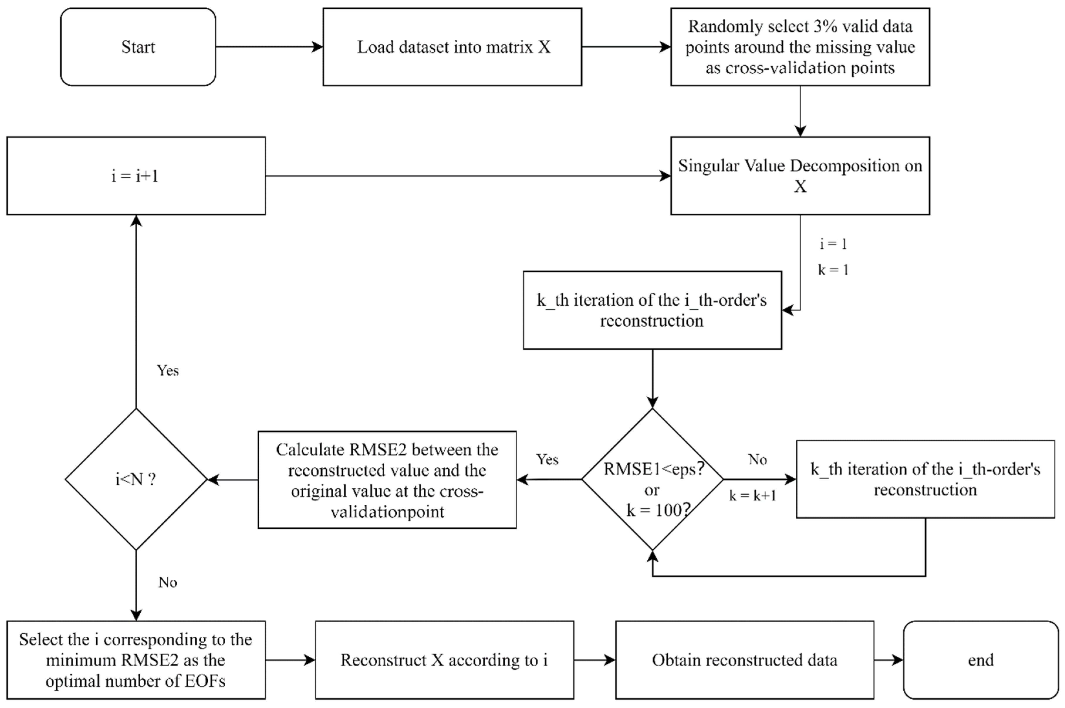
The flow chart of the IV−DINEOF algorithm is illustrated in Figure 2.

3. Data Source and Dataset Construction

Satellite remote-sensing data may have large-scale missing data due to cloud cover, satellite malfunction, image noise, etc. Thus, it is not suitable to use the original remote-sensing data to evaluate the performance of the different data reconstruction algorithms. Therefore, this paper constructs two datasets to test the improved reconstruction algorithm for the Bohai Sea of China. Dataset1 is an ideal dataset proposed by Beckers (2003) [6]. Dataset2 is a constructed dataset based on satellite remote-sensing data of sea surface temperature (SST) and chlorophyll-a (chl-a) concentration in the Bohai Sea.

3.1. Ideal Dataset (Dataset1)

Dataset1 is constructed by the same method proposed by Beckers (2003). The specific construction method is as follows:

$$\begin{array}{ll}X\left(i,j\right)=\mathit{sin}\left(x_i\right)& \mathit{sin}\left(t_j\right)+\mathit{sin}\left(2.1x_i\right)\mathit{sin}\left(2.1t_j\right)+\mathit{sin}\left(3.1x_i\right)\mathit{sin}\left(3.1t_j\right)+\mathit{tanh}\left(x_i\right)\mathit{cos}\left(t_j\right)\\ & +\mathit{tanh}\left(2x_i\right)\mathit{cos}\left(2.1t_j\right)+\mathit{tanh}\left(4x_i\right)\mathit{cos}\left(0.1t_j\right)+\mathit{tanh}\left(2.4x_i\right)\mathit{cos}\left(1.1t_j\right)+tanh\left(x_i+t_j\right)\\ & +tanh\left(x_i+2t_j\right)\end{array}$$

(2)

$x_i=2i\pi /M$,$t_j=2j\pi /N$ where i represents the row where the data point is located, j represents the column where the data point is located, M is the number of rows in the dataset, and N is the number of columns in the dataset. To avoid a loss of generality, the selected missing points are irregularly distributed and in large scale.

3.2. Constructed Dataset Based on Satellite Remote-Sensing Data (Dataset2)

The MODIS-Aqua sea surface temperature (SST) and the concentration of chlorophyll-a (chl-a) satellite remote-sensing data from 2002 to 2020 (released by NASA; the temporal resolution is 1 month, and the spatial resolution is 4 km) are used to construct the second dataset. Among them, the missing rate of the SST dataset is low, while the missing rate of the chl-a dataset is high. Therefore, the two datasets are superimposed to construct the missing SST dataset, which is called Dataset2.

The specific construction method is shown in Figure 3. Figure 3a is the original SST data, and Figure 3b is the original chl-a data. The missing area in Figure 3b is used to cover Figure 3a to obtain the structure of the constructed SST missing data, as shown in Figure 3c. The initial size of each image in Dataset2 is 93 × 118 pixels, with a total of 218 images. After excluding land points, there are 5896 spatial pixels in each image. The images and spatial points containing less than 5% are excluded in the analysis because they do not provide useful information and might affect the final result [20]. Finally, there are 5747 effective spatial pixels in each frame of the image.

4. Performance of IV−DINEOF Algorithm

4.1. Verification Metrics

Referring to Ping (2015), five statistical metrics—correlation coefficient (r), root mean square error (RMSE), signal-to-noise ratio (SNR), mean absolute difference (MAD) and, structural similarity (SSIM)—are selected to test the performance of the IV−DINEOF algorithm [3]. The complete dataset X generated by Equation (2) can be used to construct Dataset1, so SSIM is used only to evaluate Dataset1.

The correlation coefficient is the Pearson correlation coefficient, and the signal-to-noise ratio (SNR) is the ratio of the reconstructed data’s standard deviation to the error’s standard deviation (the difference between the reconstructed data and the original data). The five statistical metrics are defined as follows:

$$\begin{array}{c}r=\frac{1}{n-1}{\displaystyle {\displaystyle \sum }_{i=1}^n}\left(\frac{S_i-{\mu }_S}{{\sigma }_S}\right)\left(\frac{I_i-{\mu }_I}{{\sigma }_I}\right)\end{array}$$

(3)

$$\begin{array}{c}RMSE=\sqrt{\frac{{\displaystyle \sum }{\left(S-I\right)}^2}{n}}\end{array}$$

(4)

$$\begin{array}{c}SNR=\frac{{\sigma }_I}{{\sigma }_{S-I}}\end{array}$$

(5)

$$\begin{array}{c}MAD=\frac{{\displaystyle \sum }\left|S-I\right|}{n}\end{array}$$

(6)

$$\begin{array}{c}SSIM=\frac{\left(2{\mu }_S{\mu }_I+c_1\right)\left(2{\sigma }_{SI}+c_2\right)}{\left({\mu }_S^2+{\mu }_I^2+c_1\right)\left({\sigma }_S^2+{\sigma }_I^2+c_2\right)}\end{array}$$

(7)

where S is the original data, I is the reconstructed data, and $n$ is the corresponding number of samples. ${\mu }_S$ and ${\mu }_I$ are the mean of the original data and the mean of the reconstructed data, respectively. ${\sigma }_S$, ${\sigma }_I$, and ${\sigma }_{S-I}$ are the standard deviation of the original data, the standard deviation of the reconstructed data, and the standard deviation of the difference between the reconstructed and original data, respectively. ${\sigma }_{SI}$ is the covariance of $S$ and $I$. ${\sigma }_S^2$ and ${\sigma }_I^2$ are the variances of $S$ and $I$, respectively. In Equation (7), $c_1={\left(k_{1}L\right)}^2$ and $c_2={\left(k_{2}L\right)}^2$, where $k_1=0.01$ and $k_2=0.03$. $L$ is the dynamic range of the pixel values, but in this paper, $L=S_{max}-S_{min}$.

The above statistical metrics are used to compare the reconstruction results of the DINEOF algorithm, the IV−DINEOF algorithm, and VE−DINEOF algorithm to evaluate the performance of the three algorithms.

4.2. Reconstruction Results of Dataset1

Table 1. Comparison of mean values of verification metrics among DINEOF, IV−DINEOF, and VE−DINEOF for Dataset1.

Verification Metrics	r	SNR	RMSE	MAD	SSIM	Average Number of Iterations
DINEOF	0.8919	2.7401	0.7873	0.3831	0.3289	7071
IV−DINEOF	0.9225	3.4502	0.6609	0.3125	0.3334	6776
VE−DINEOF	0.8713	1.7867	0.8821	0.4322	0.3237	2563

shows the mean values of the verification metrics for 300 different missing cases of Dataset1 constructed by the DINEOF algorithm, the IV−DINEOF algorithm, and the VE−DINEOF algorithm, respectively.

As can be seen from Table 1, compared with the DINEOF algorithm, the IV−DINEOF algorithm improves the $r$ and SNR of the reconstruction results from 0.8919 and 2.7401 to 0.9225 and 3.4502, respectively. The RMSE and MAD were reduced from 0.7873 and 0.3831 to 0.6609 and 0.3125, respectively. There is no significant difference in the values of SSIM, which are 0.3289 and 0.3334, respectively. For the VE−DINEOF algorithm, the reconstruction performance is inferior to the other two algorithms. As the calculation time depends on CPU speed, memory capacity, program code, etc., this paper does not compare the computational time. Instead, the number of iterations is used to evaluate the computational efficiency of the three algorithms. Among these three algorithms, the VE−DINEOF algorithm is the one with the shortest computation time, and the average number of iterations is only 2563. The average number of iterations of the DINEOF algorithm and the IV−DINEOF algorithm are 7071 and 6776, respectively. Therefore, it can be shown that the computational time of these two algorithms (DINEOF and IV−DINEOF) are basically the same, even when the computational time of the IV−DINEOF algorithm is slightly shorter than the DINEOF algorithm, and the reconstruction accuracy of the IV−DINEOF algorithm is improved significantly.

4.3. Comparison of the Reconstruction Performance for Different Rates of Missing Data

To better verify the accuracy of the IV−DINEOF algorithm and the reconstruction performance under different overall missing rates, this paper compares data under three different overall missing rates, which are 20%, 40%, and 60% (representing cases with low deficiency, moderate deficiency, and large deficiency, respectively).

Table 2. Comparison of verification metrics among DINEOF, IV−DINEOF, and VE−DINEOF for different overall missing rates in Dataset1.

Overall Missing Rate	Algorithm	r	SNR	RMSE	MAD	SSIM
20%	DINEOF	0.9818	25.9378	0.2678	0.0635	0.3335
	IV−DINEOF	0.9916	35.8065	0.1553	0.0348	0.3337
	VE−DINEOF	0.9531	3.2707	0.5336	0.1691	0.3358
40%	DINEOF	0.9358	4.4649	0.5850	0.2387	0.3331
	IV−DINEOF	0.9518	4.9534	0.5048	0.1995	0.3350
	VE−DINEOF	0.8900	1.9148	0.8271	0.3874	0.3300
60%	DINEOF	0.8992	2.2693	0.7654	0.3706	0.3288
	IV−DINEOF	0.9015	2.2557	0.7641	0.3667	0.3292
	VE−DINEOF	0.8530	1.5783	0.9398	0.5044	0.3207

shows the comparison of statistical metrics among the DINEOF, IV−DINEOF, and VE−DINEOF algorithms for different overall missing rates.

Compared with the DINEOF algorithm, when the missing rate is 20%, the IV−DINEOF algorithm increases the r and SNR of the reconstructed result from 0.9818 and 25.9378 to 0.9916 and 35.8065, respectively. The RMSE and MAD were reduced from 0.2678 and 0.0635 to 0.1553 and 0.0348, respectively.

When the missing rate rises to 40%, the IV−DINEOF algorithm increases the r and SNR of the reconstruction results from 0.9358 and 4.4649 to 0.9518 and 4.9534, respectively. The RMSE and MAD decreased from 0.5850 and 0.2387 to 0.5048 and 0.1995, respectively.

When the missing rate reaches 60%, the IV−DINEOF algorithm increases the r from 0.8992 to 0.9015. The SNRs of the two algorithms are 2.2693 and 2.2557, respectively, which are almost the same. The RMSE and MAD decreased from 0.7654 and 0.3706 to 0.7641 and 0.3667, respectively. However, the difference in the SSIM is not significant, regardless of the rate of missing data.

Compared with the VE−DINEOF algorithm, the verification metrics, except for SSIM, of the IV−DINEOF and DINEOF algorithms are always better than the VE−DINEOF algorithm, regardless of the missing rate. Since the VE−DINEOF algorithm has variable optimal EOFs during reconstruction, this may lead to the situation where the EOFs selected in one iteration step during the algorithm execution are not the optimal EOFs for this iteration, making the final reconstruction results unsatisfactory.

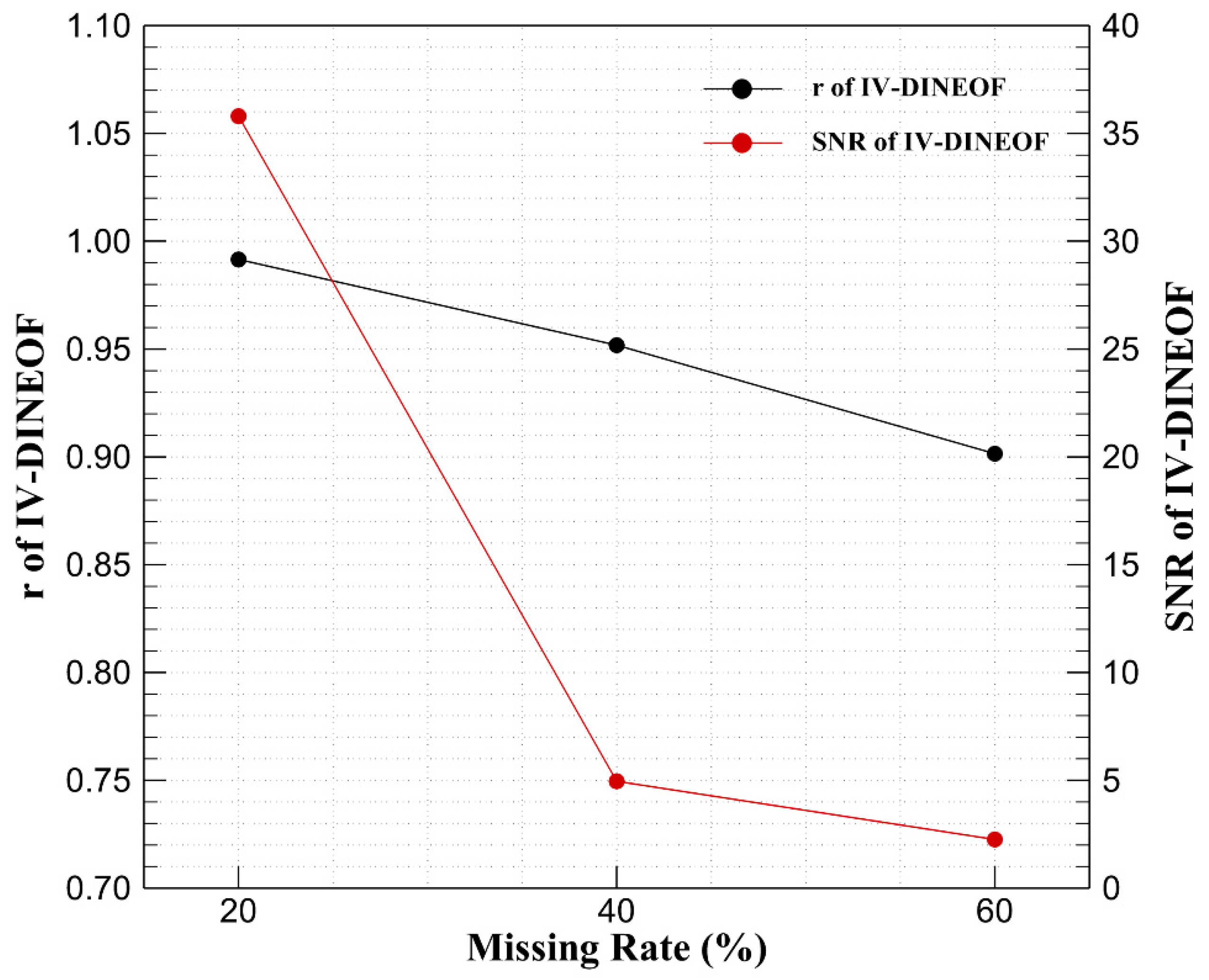
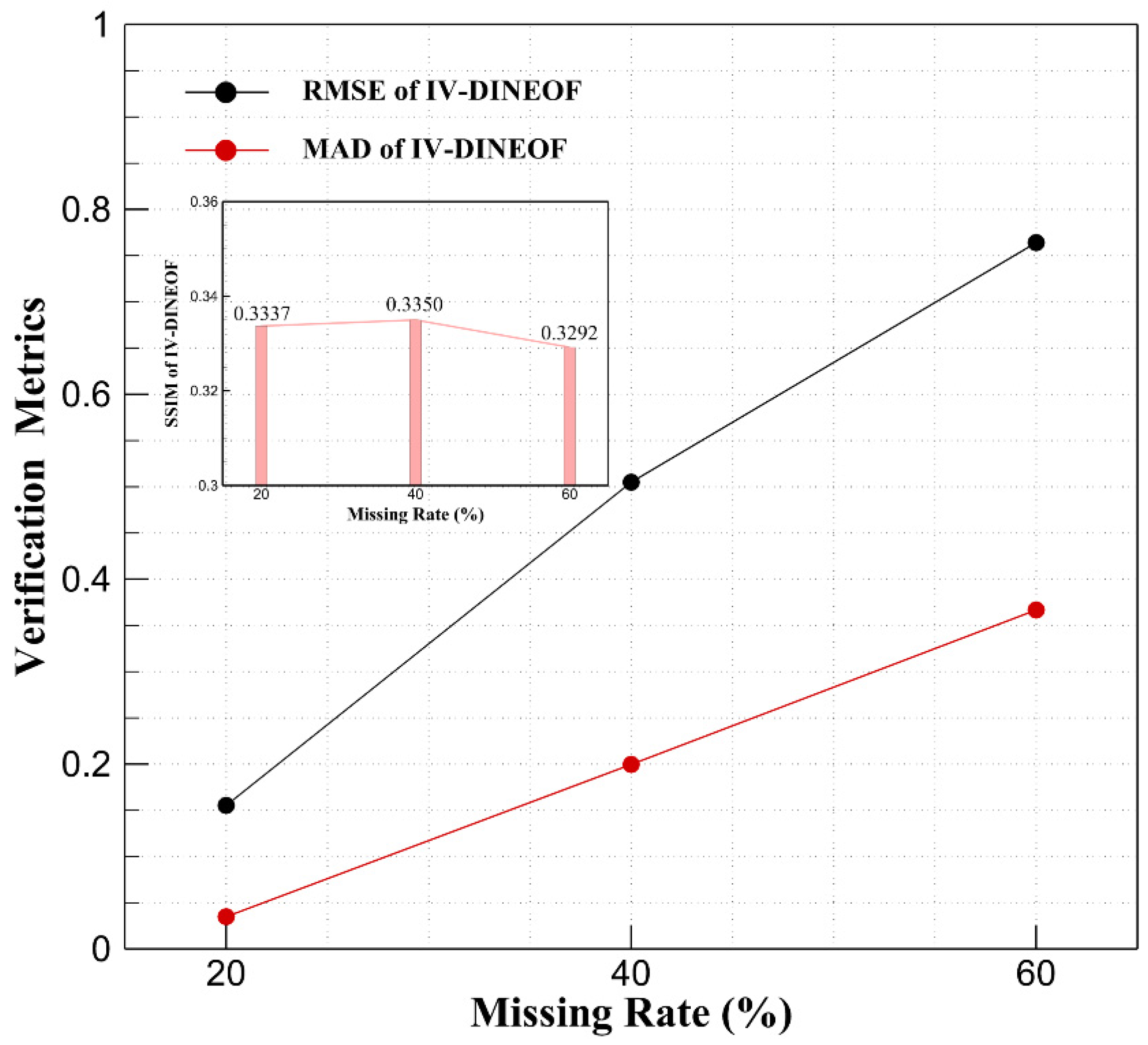
Figure 4 and Figure 5 show the changes in the verification metrics of the IV−DINEOF algorithm as the missing rate changes. It can be seen from Figure 4 and Figure 5 that the correlation coefficient and signal-to-noise ratio of the IV−DINEOF algorithm decrease with the increase of the overall missing rate.

The root mean square error and the mean absolute difference have the same trend, both decreasing as the overall missing rate increases. The change in SSIM appears to be independent of the overall rate of missing data. Although the correlation coefficient and the signal-to-noise ratio decrease with the increase of the overall missing rate, the performance of the IV−DINEOF algorithm is still better than that of the DINEOF algorithm.

4.4. Reconstruction Results of Dataset2

Table 3. Comparison of verification metrics between DINEOF and IV−DINEOF for Dataset2.

Verification Metrics	r	SNR	RMSE	MAD	Number of Iterations
DINEOF	0.8833	1.8598	4.4152	2.4008	2.1919
IV−DINEOF	0.9378	2.6805	3.2955	1.6278	2.1919

presents the evaluation of the overall reconstruction results for the Dataset2 dataset. It can be seen from Table 3 that under the same number of iterations, the IV−DINEOF algorithm increases the r and SNR of the reconstruction results of the SST missing dataset from 0.8833 and 1.8598 to 0.9378 and 2.6805, respectively. The RMSE and MAD were reduced from 4.4152 and 2.4008 to 3.2955 and 1.6278, respectively.

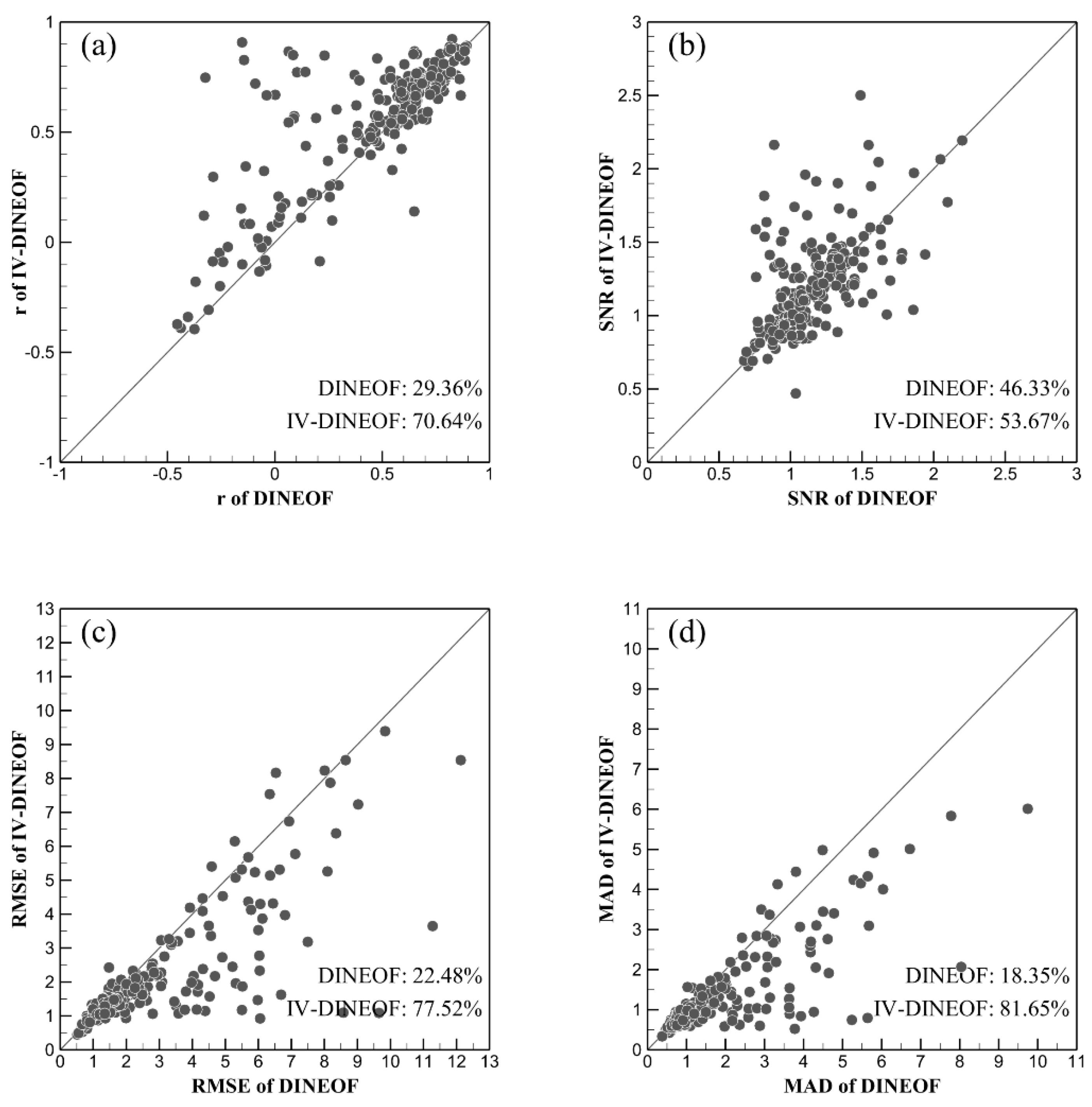
Figure 6 shows the evaluation of the reconstruction results for every single month of the Dataset2, which includes the correlation coefficient (Figure 6a), signal-to-noise ratio (Figure 6b), root mean square error (Figure 6c), and mean absolute difference (Figure 6d) of the DINEOF algorithm and the IV−DINEOF algorithm.

After reconstruction using the IV−DINEOF algorithm, the r in most months is higher than the result of reconstruction using the DINEOF algorithm (Figure 6a). Among them, there were 154 months in which the IV−DINEOF algorithm was superior to the DINEOF algorithm in terms of the correlation coefficient, accounting for 70.64% of the total months.

The SNR of the reconstruction result of the IV−DINEOF algorithm is slightly better than that of the reconstruction result using the DINEOF algorithm (Figure 6b). Among them, there were 117 months in which the IV−DINEOF algorithm was superior to the DINEOF algorithm in terms of signal-to-noise ratio, accounting for 53.67% of the total months.

Figure 6c shows that after reconstruction using the IV−DINEOF algorithm, the RMSE of most months is lower than the result of reconstruction using the DINEOF algorithm. Among them, there are 169 months in which the IV−DINEOF algorithm is better than the DINEOF algorithm in terms of root mean square error, accounting for 77.52% of the total months.

For the MAD indicator, the reconstruction using the IV−DINEOF algorithm resulted in a lower MAD for most months than the reconstruction using the DINEOF algorithm (Figure 6d). Among them, there are 178 months in which the IV−DINEOF algorithm is superior to the DINEOF algorithm in terms of mean absolute difference, accounting for 81.65% of the total.

Table 4. Comparison of verification metrics of reconstruction results between DINEOF and IV−DINEOF with different single-month missing rates using Dataset2.

Month	Missing Rate	Verification Metrics	r	SNR	RMSE	MAD
Feb. 2003	19.56%	DINEOF	0.1922	1.0189	5.9978	4.1773
		IV−DINEOF	0.5644	1.1512	3.5289	2.4369
Jul. 2010	41.11%	DINEOF	−0.1527	0.8846	8.5714	5.2358
		IV−DINEOF	0.9075	2.1632	1.1000	0.7468
Jun. 2013	57.19%	DINEOF	0.3934	0.8863	2.4923	1.4579
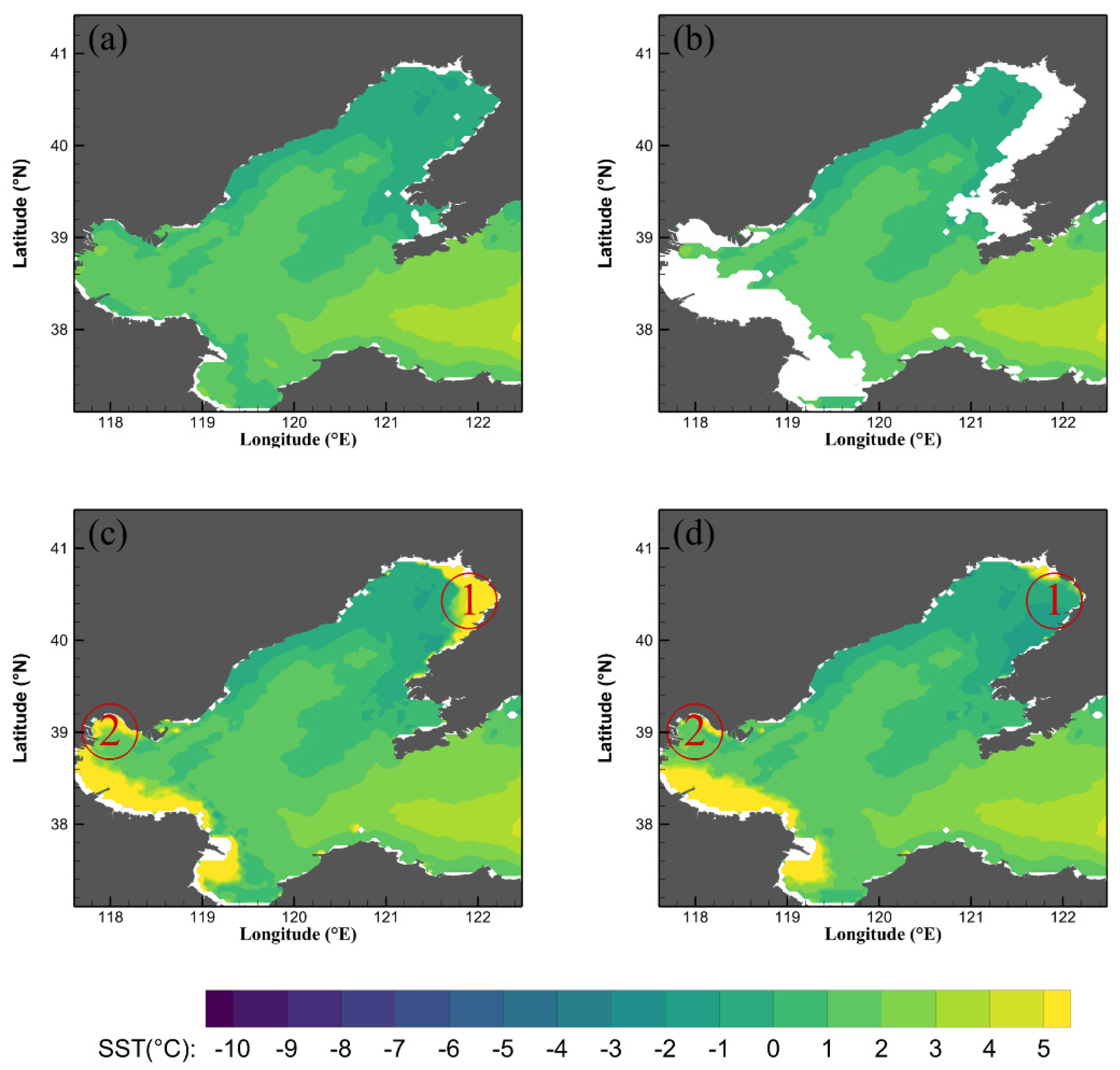
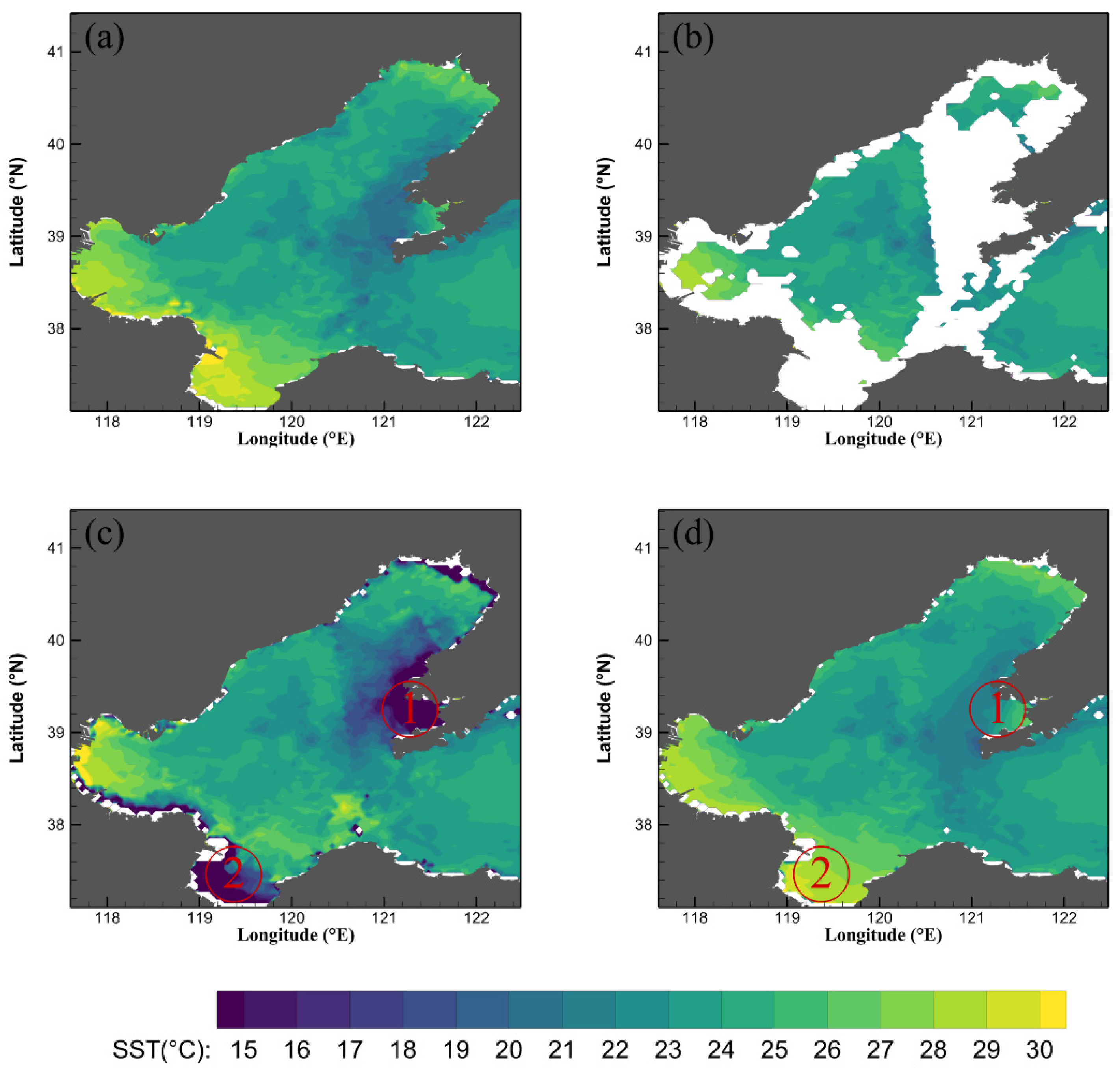
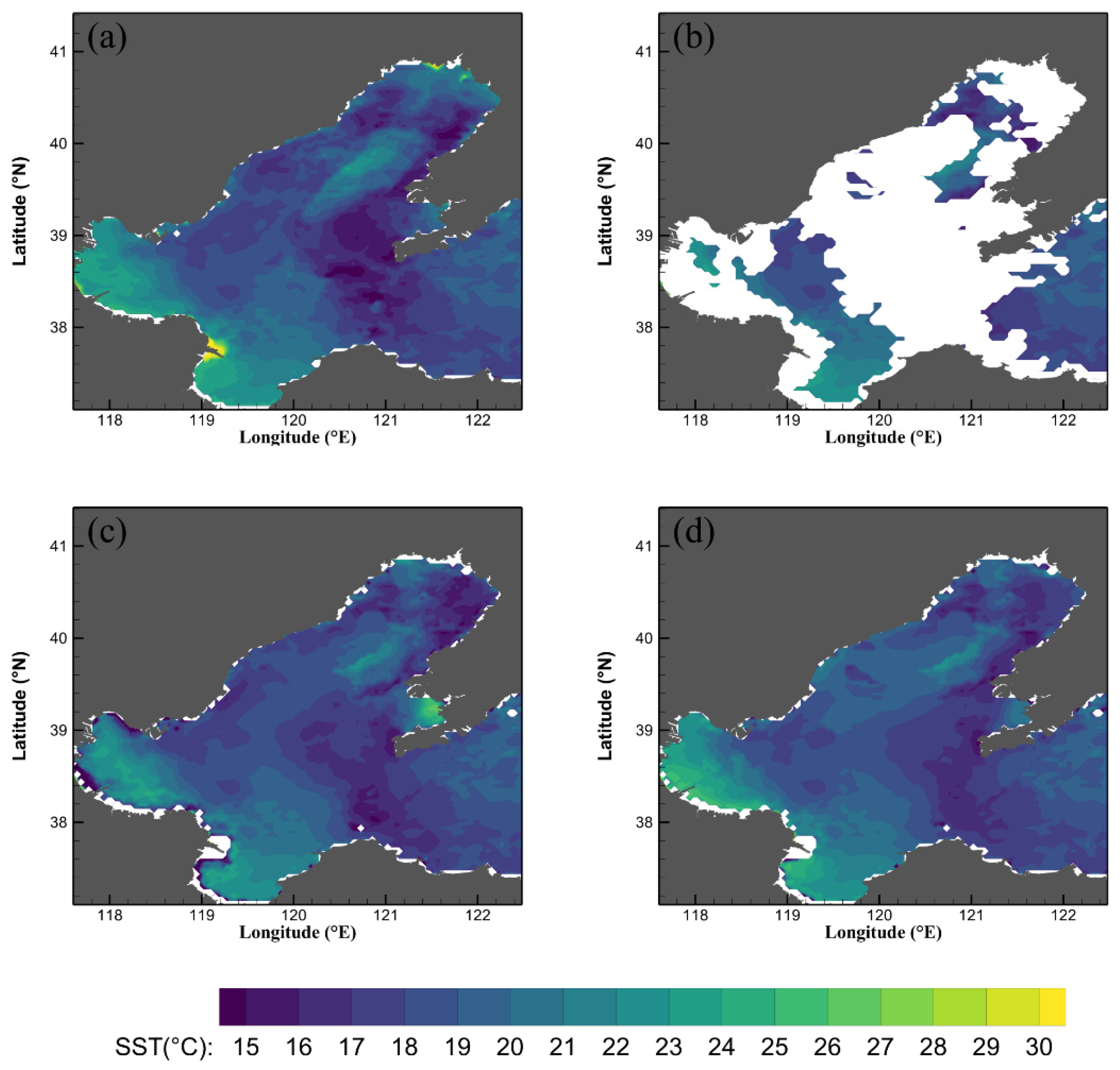
		IV−DINEOF	0.7350	1.3311	1.6238	1.0983

compares the reconstruction results between the DINEOF algorithm and the IV−DINEOF algorithm for the February 2003 (missing rate 19.56%), July 2010 (missing rate 41.11%), and June 2013 (missing rate 57.19%) data. Figure 7, Figure 8 and Figure 9 show the reconstruction results of the three months, respectively.

Compared with the DINEOF algorithm, in the February 2003 data, the IV−DINEOF algorithm increased the r and SNR of the reconstruction results from 0.1922 and 1.0189 to 0.5644 and 1.1512, respectively. The RMSE and MAD were reduced from 5.9978 and 4.1773 to 3.5289 and 2.4369, respectively (Table 4). Comparing Figure 7a,c,d, the reconstruction results of the IV−DINEOF algorithm are better than those of the DINEOF algorithm in Area 1 (i.e., the north-eastern part of Liaodong Bay) and Area 2 (i.e., the western part of Bohai Bay).

Compared with the DINEOF algorithm for the July 2010 data, the r of the IV−DINEOF algorithm was improved from −0.1527 to 0.9075, while the SNR was improved from 0.8846 to 2.1632; the RMSE and the MAD decreased from 8.5714 and 5.2358 to 1.1 and 0.7468, respectively. From Figure 8a,d, it can be seen that the reconstruction result of the IV−DINEOF algorithm is almost the same as the original data. However, Figure 8c shows that the result of the DINEOF algorithm is not satisfied; specifically, there exist more extreme values in Area 1, Area 2, and along the shoreline.

Compared with the result of the DINEOF algorithm for the June 2013 data, the r and SNR of the IV−DINEOF algorithm increased from 0.3934 and 0.8863 to 0.7350 and 1.3311, respectively; the RMSE and the MAD were reduced from 2.4923 and 1.4579 to 1.6238 and 1.0983, respectively. Comparing Figure 9a,c,d, it can be seen that the reconstruction results of the IV−DINEOF algorithm and the DINEOF algorithm are the same, but the DINEOF algorithm has more extreme values in the data along the shoreline.

5. Discussion

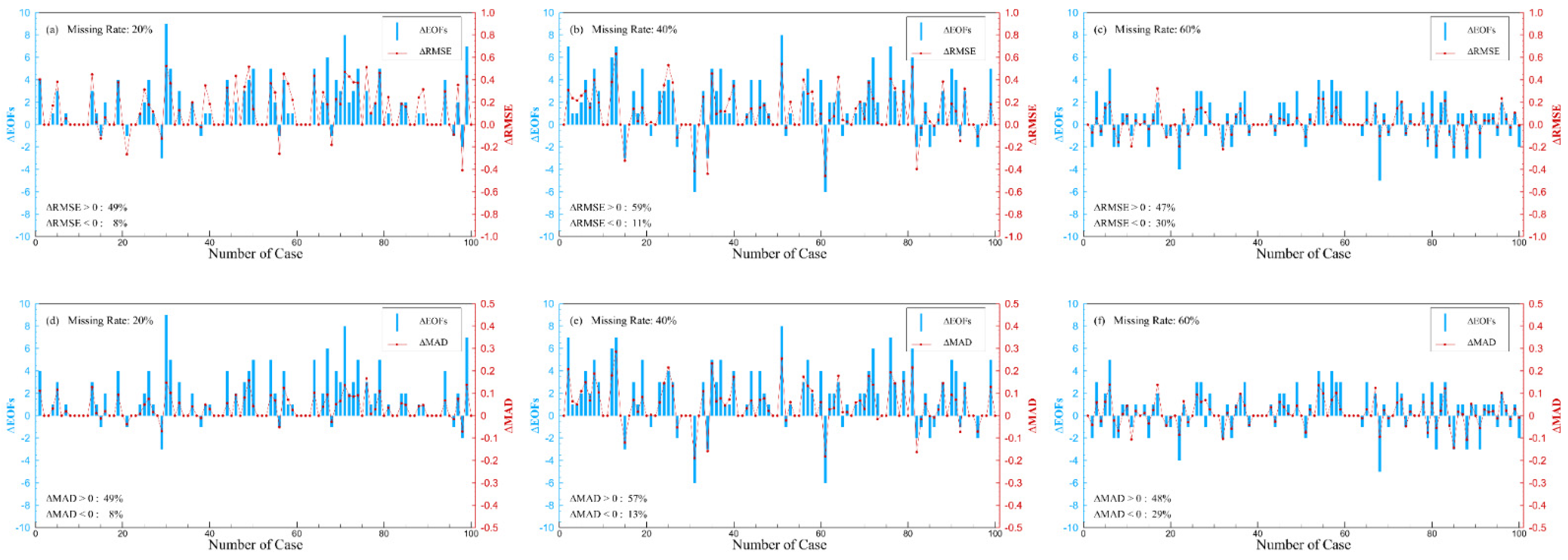
In this study, 100 sets, each having missing data at the rates of 20%, 40%, and 60%, were constructed using the complete data set X generated by Equation (2). Then, the missing datasets were reconstructed using the DINEOF algorithm and the IV−DINEOF algorithm, respectively.

Figure 10 and Figure 11 present the difference between the optimal EOFs selected by the DINEOF algorithm and the improved algorithm under different missing rates and the difference between the two algorithms in five validation indexes (i.e., r, RMSE, SNR, MAD, and SSIM). The difference of optimal EOFs (∆EOFs) is determined by Equation (8), and the differences of the validation metrics (correlation coefficient difference ∆r, root mean square error difference ∆RMSE, signal-to-noise ratio difference ∆SNR, mean absolute difference ∆MAD, and structural similarity index difference ∆SSIM) are determined by the following Equations (9)–(13).

$$\begin{array}{c}\Delta EOFs=EOF{s}_{DINEOF}-EOF{s}_{IV-DINEOF}\end{array}$$

(8)

$$\begin{array}{c}\Delta r=r_{DINEOF}-r_{IV-DINEOF}\end{array}$$

(9)

$$\begin{array}{c}\Delta RMSE=RMS{E}_{DINEOF}-RMS{E}_{IV-DINEOF}\end{array}$$

(10)

$$\begin{array}{c}\Delta SNR=SN{R}_{DINEOF}-SN{R}_{IV-DINEOF}\end{array}$$

(11)

$$\begin{array}{c}\Delta MAD=MA{D}_{DINEOF}-MA{D}_{IV-DINEOF}\end{array}$$

(12)

$$\begin{array}{c}\Delta SSIM=SSI{M}_{DINEOF}-SSI{M}_{IV-DINEOF}\end{array}$$

(13)

5.1. Optimal EOFs and SSIM

The selection of the optimal EOFs usually affects the reconstructed data quality. Figure 10 (blue bar) shows that the optimal EOFs selected by the improved algorithm are mostly lower than the optimal EOFs determined by the DINEOF algorithm. At low missing rates (20%), only in 8% of the cases, the optimal EOFs of the DINEOF algorithm are lower than the optimal EOFs of the improved algorithm. When the missing rate increases to 40%, the percentage of cases in which the optimal EOFs of the DINEOF algorithm are lower than the optimal EOFs of the improved algorithm rises to 14%. When the missing rate is at a high level (60%), the number of cases in which the optimal EOFs of the DINEOF algorithm are lower than the optimal EOFs of the improved algorithm also rises to 39%.

The difference in structural similarity metrics between the two algorithms is not significant (Figure 10a–c), fluctuating between ±0.05. The difference in structural similarity metrics between the two algorithms fluctuates in the ±0.05 interval (Figure 10a–c). This indicates that the reconstructed data obtained using the DINEOF algorithm and the IV−DINEOF algorithm are at comparable levels in terms of SSIM. When the dataset is at a low overall missing rate (Figure 10a), the SSIM of the improved algorithm is essentially comparable to that of the original algorithm. The SSIM difference fluctuates as the missing rate increases, but the fluctuation range is basically within the ±0.05 interval, and it can be assumed that there is no gap between the two algorithms in this metric of SSIM.

5.2. r and SNR

As shown in Figure 10d–f, the correlation coefficient difference (∆r) varies with the optimal EOFs difference (∆EOFs). This means that when reconstructing the same missing data set, the two algorithms determine their respective optimal EOFs, and the algorithm corresponding to the lower optimal EOFs can obtain reconstructed data with higher correlation coefficients. When the missing rate is 20%, the positive or negative of ∆r depends entirely on ∆EOFs. ∆r tends to be smaller than zero when ∆EOFs is larger than zero. When the missing rate increases to 40% and 60%, some cases appear where the larger optimal EOFs reconstruct the data with higher correlation coefficient values; however, the frequency of such cases is within 5%. In terms of statistical significance, it can still be considered that lower optimal EOFs have better reconstruction effects in terms of reconstructing data correlation coefficients.

Similar to the correlation coefficients, choosing lower optimal EOFs for reconstruction also results in higher SNR values (Figure 10g–i), while individual cases of higher EOFs obtaining higher SNRs also occur as the overall missing rate grows.

5.3. RMSE and MAD

The RMSE and MAD metrics reflect the error between the reconstructed and original data, so higher values indicate less satisfactory reconstruction quality. As shown in Figure 11a–c, when the missing rate is low, the positive and negative of ∆RMSEs are consistent with the ∆EOFs. With the increase in the missing rate, there are also some cases where the positive and negative of ∆RMSEs are different from the ∆EOFs; however, these cases account for less than 5% of the total number of cases. MAD shows the same situation as RMSE.

On the basis of the above results, it can be assumed that higher-order modes are introduced into the reconstructed data when higher optimal EOFs are used to reconstruct the data. However, the proportion of valid information in these introduced higher-order modes is very low and contains a large amount of error information due to the setting of missing data initial values, which makes the data reconstruction effect unsatisfactory. The optimal EOFs determined by the IV−DINEOF algorithm during data reconstruction are always lower than the optimal EOFs determined by the original algorithm, thus making the reconstruction effect of the IV−DINEOF algorithm better than that of the original IDNEOF algorithm. This is most likely due the IV−DINEOF algorithm making full use of the valid information around the missing values points when selecting the cross-validation points such that the lower optimal EOFs can be selected, thus avoiding the introduction of errors contained in higher-order modes. More rigorous mathematical analysis needs further study.

6. Conclusions

On the basis of Beckers’ (2003) DINEOF algorithm, an improved DINEOF algorithm (IV−DINEOF) is proposed in this paper, in which a new method is proposed to select the cross-validation points [6]. The IV−DINEOF algorithm can choose lower optimal EOFs to reduce the error information caused by the introduction of higher-order modes since the improved cross-validation point selection approach can effectively reflect the data characteristics around the missing values. In addition, it also avoids the excessive aggregation of the cross-validation points. The performance of the improved algorithm has been tested with two sets of data, and the results showed that: (1) the correlation coefficient (r), root mean square error (RMSE), signal-to-noise ratio (SNR), and mean absolute difference (MAD) of the IV−DINEOF algorithm are all superior to those of the original DINEOF and the VE−DINEOF algorithms; (2) better reconstruction outcomes are achieved with lower optimal EOFs; and (3) there is no significant difference in SSIM metrics among these three algorithms.

The validation-point selection method proposed in this paper is applied only to the IV−DINEOF algorithm, so this selection method can be combined with other improved DINEOF algorithms for future applications, while more rigorous mathematical analysis needs further study.