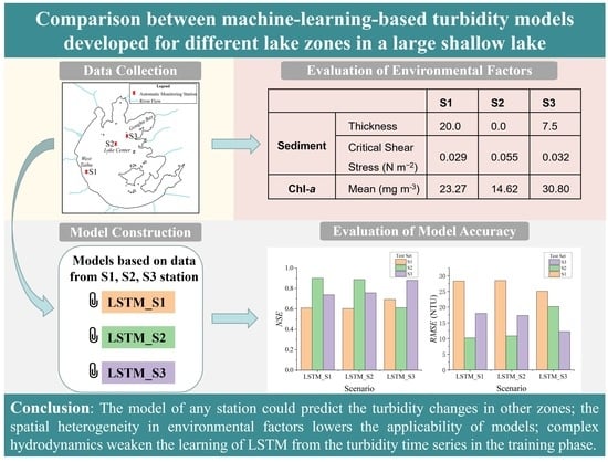
Comparison between Machine-Learning-Based Turbidity Models Developed for Different Lake Zones in a Large Shallow Lake

Abstract

Machine learning has been used to mine the massive data collected by automatic environmental monitoring systems and predict the changes in the environmental factors in lakes. However, further study is needed to assess the feasibility of the development of a universal machine-learning-based turbidity model for a large shallow lake with considerable spatial heterogeneity in environmental factors. In this study, we collected and examined sediment and water quality data from Lake Taihu, China. Three monitoring stations were established in three lake zones to obtain continuous time series data of the water quality and meteorological variables. We used these data to develop three turbidity models based on long short-term memory (LSTM). The three zones differed in terms of environmental factors related to turbidity: in West Taihu, the Lake Center, and the mouth of Gonghu Bay, the critical shear stress of bed sediments was 0.029, 0.055, and 0.032 N m⁻², and the chlorophyll-a concentration was 23.27, 14.62, 30.80 μg L⁻¹, respectively. The LSTM-based turbidity model developed for any zone could predict the turbidity in the other two zones. For the model developed for West Taihu, its performance to predict the turbidity in the local zone (i.e., West Taihu) was inferior to that for the other zones; the reverse applied to the models developed for the Lake Center and Gonghu Bay. This can be attributed to the complex hydrodynamics in West Taihu, which weakens the learning of LSTM from the time series data. This study explores the feasibility of the development of a universal LSTM-based turbidity model for Lake Taihu and promotes the application of machine learning algorithms to large shallow lakes.

1. Introduction

Turbidity is a measure of the decrease in water clarity due to insoluble substances. Decreased translucency due to increased turbidity impairs both the landscape value and light-dependent biogeochemical processes of lakes [1,2]. Therefore, turbidity is an important indicator of the quality of lake environments [3], and is included in almost all automatic lake environment monitoring systems. Although the importance of turbidity has been widely recognized and large volumes of turbidity data have been collected, few studies have focused on using other environmental factors to predict turbidity. Turbidity is a composite water quality indicator that integrates the characteristics of sediments, humus, algae, colloids, and other particles in lake water [4]. It is strongly nonlinear; therefore, it is difficult to accurately simulate turbidity changes in lakes using regression models [5].

Having benefited from the developments of computer technology and science in recent years, machine learning has been widely applied to the field of environmental science and has significantly improved the interpretation of environmental monitoring data and the prediction accuracy of complex environmental factors [6,7]. Artificial neural networks [8,9,10,11], such as backpropagation neural networks [12] and recurrent neural networks [13], have been frequently used to predict lake environmental factors using the massive volumes of data collected by environmental monitoring programs. The long short-term memory (LSTM) model, which is a type of recurrent neural network, is particularly suitable for time series data [14], and is one of the most popular machine learning methods for predicting environmental factors, such as water level [15], dissolved oxygen [16], chlorophyll-a concentration [17], and turbidity [18], in lakes.

However, it is necessary to evaluate the differences between the machine-learning-based turbidity models developed for different zones in a large lake [19]. A machine-learning-based model is usually trained based on the data from a single field station. However, the environmental factors in a large lake usually exhibit large temporal and spatial variations, and the data from a single station may not be representative of the conditions of all of the zones in the lake. For example, the critical shear stress of sediments varies spatially because of the spatial heterogeneity of the physicochemical properties of sediments in large lakes [20], which in turn impacts the spatiotemporal distribution of the suspended sediment concentration [21]. In a large shallow lake that is susceptible to algal blooms, the turbidity may be affected by the spatial heterogeneity of algal particulates [22]. Theoretically, machine-learning-based models are point-based and are unable to take into account such heterogeneities [23]. Few studies have focused on the adaptability of the models that are trained using the data from a single field station. Therefore, in this study, we examine the applicability of these models to predict the turbidity in different zones of large lakes.

For this study, three high-frequency field stations were established in three zones of Lake Taihu, China, to obtain continuous time series data of the water quality and meteorological variables. We used these time series data and developed three LSTM-based turbidity models to simulate the turbidity changes in the three zones; we compared the accuracy of the simulation results from the different models. Our main objectives are: (1) to study the differences in performance between the LSTM-based turbidity models trained by the time series data collected from different zones of Lake Taihu; and (2) to explore the feasibility of the development of a universal LSTM-based turbidity model for this large shallow lake.

2. Materials and Methods

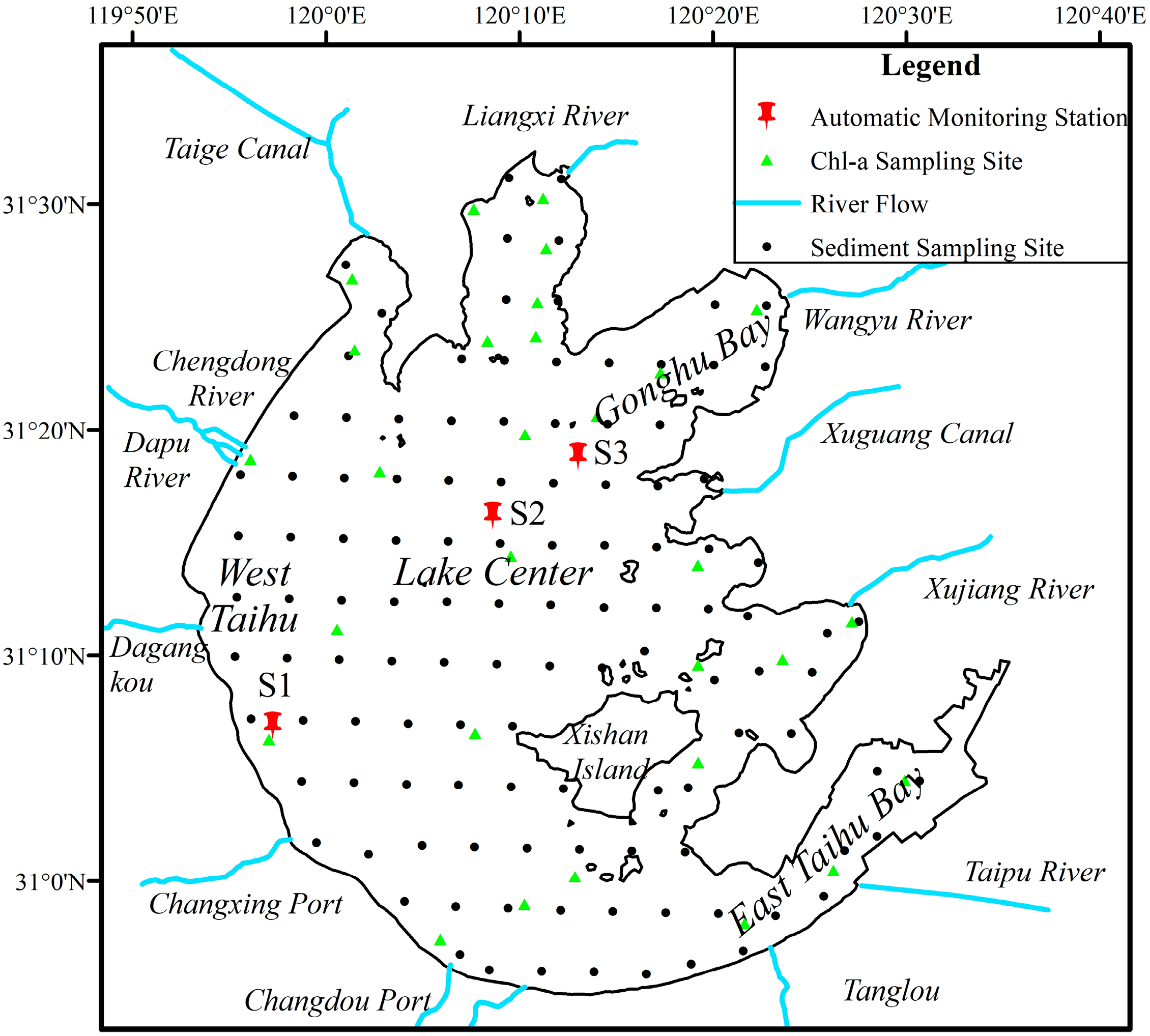
2.1. Study Area

Lake Taihu, located in the economically developed and densely populated middle and lower reaches of the Yangtze River in China, has a surface area of approximately 2338 km². It is a typical large shallow lake, with an average depth of 1.9 m and a maximum depth of less than 3 m [24]. The Lake Taihu basin is in a subtropical monsoon climate zone, with southeasterly winds prevailing in summer and autumn and northwesterly winds prevailing in winter and spring [24]. Studies have shown that the wind field has an important influence on the turbidity of Lake Taihu [25]. The inflows are mainly on the western lakeshore, while the outflows are on the eastern lakeshore (Figure 1). The inflows carry a large number of upstream sediments into Lake Taihu and result in the silting up of West Taihu. In addition, Lake Taihu suffers from severe eutrophication and cyanobacterial blooms occur frequently in the northwestern part of the lake between April and October every year [26].

2.2. Data Collection

2.2.1. Sediment and Chlorophyll-a

The sediments were collected and examined at 116 sediment sampling sites (Figure 1) distributed across Lake Taihu. At each site, the thickness of the sludge was measured using the rod measurement method [27], samples of the uppermost sediments (about 50 g) were collected for physical and chemical analyses, and the latitude and longitude were recorded. The Taihu Laboratory for Lake Ecosystem Research provided monthly lab-based chlorophyll-a (Chl-a) concentrations at all of the chlorophyll-a sampling sites (Figure 1) for 2017–2021, and analyzed the density and the moisture content of the sediments.

2.2.2. High-Frequency In Situ Observations

We established three environmental monitoring stations along a southwest-northeast transect across Lake Taihu. The water quality and meteorological data were automatically collected at the stations located in West Taihu (S1), Lake Center (S2), and the mouth of Gonghu Bay (S3) (Figure 1). At each station, a YSI-6600 Sonde (YSI Inc., Yellow Springs, OH, USA) was installed 1 m below the lake surface: it measured the water temperature (0.001 °C), conductivity (0.01 mS cm⁻¹), pH (0.01), chlorophyll-a (0.01 ug/L⁻¹), phycocyanin (0.01 ug/L⁻¹), dissolved oxygen (0.01 mg L⁻¹), and turbidity (0.1 NTU). At each station, a portable weather station WXT520 (Vaisala, Finland) was installed 4 m above the lake surface: it measured the wind speed (0.1 m s⁻¹), temperature (0.1 °C), relative humidity (0.1%), and pressure (0.1 hPa). Sondes were calibrated weekly. Sampling interval was 30 min for both Sonde and WX520.

2.3. LSTM-Based Turbidity Model

2.3.1. LSTM

The LSTM is a special type of recurrent neural network [14]. It has three different types of gates: the forget gate, input gate, and output gate. The forget gate is responsible for discarding or retaining information; the input gate is responsible for updating the state of the neural cell; and the output gate is responsible for determining the value of the hidden state that is input to the next neural cell. Therefore, the LSTM model can remember important information from earlier time steps without being affected by short-term memory [28]. In machine learning, the vanishing gradient problem could be encountered when training artificial neural networks with gradient-based learning methods and backpropagation [29]. In such methods, during each iteration of training, each of the neural network’s weights receives an update proportional to the partial derivative of the error function with respect to the current weight. The LSTM is able to effectively avoid such a problem and is better at learning long-term sequence data.

2.3.2. Development of LSTM-Based Turbidity Model

For each station, each raw time series dataset (e.g., wind speed or turbidity) was normalized and transformed into a supervised learning dataset using walk-forward validation [30] (Figure 2). The transformed dataset was further split into a training set, a validation set and a test set, which were used for training, evaluation, and error detection, respectively. During data processing, the input time window (2–16 h) and the size of the training set (600–9000 sets) were adjusted continuously to determine the optimum solution for the initial input data.

Using TensorFlow (Mountain View, CA, USA), we developed and applied three LSTM-based turbidity models: LSTM_S1, LSTM_S2, and LSTM_S3 were based on the time series data from the sites S1, S2, and S3, respectively.

2.3.3. LSTM Model Experiments

We designed different wind field scenarios (LSTM_W,

Table 1. Wind field (LSTM_W) and station (LSTM_S) scenarios used in model experiments.

Scenario	Prediction	Future Wind Speed	Train Set	Test Set
LSTM_W	LSTM_S2-W1	No	S2	S2
	LSTM_S2-W2	Yes	S2	S2
LSTM_S	LSTM_S11, S12, S13	Yes	S1	S1, S2, S3
	LSTM_S21, S22, S23	Yes	S2	S1, S2, S3
	LSTM_S31, S32, S33	Yes	S3	S1, S2, S3

Remark: S1, S2, and S3 represent the dataset comprising raw data collected at stations S1, S2, and S3, respectively.

) to evaluate the influence of the wind speed on the performance of the LSTM-based turbidity models. We used the model based on the time series data collected from Station S2 (LSTM_S2); LSTM_S2-W1 is the model prediction that omits the future wind speed and LSTM_S2-W2 is the model prediction that takes into account the future wind speed.

We designed station scenarios (LSTM_S, Table 1) to assess the differences between LSTM_S1, LSTM_S2, and LSTM_S3. We used LSTM_S1 to predict the turbidity at stations S1, S2, and S3; LSTM_S11, S12, and S13 are the model predictions for S1, S2, and S3, respectively. Similarly, LSTM_S21, S22, and S23 are the predictions of LSTM_S2 for S1, S2, and S3; LSTM_S31, S32, and S33 are the predictions of LSTM_S3. We examined and compared the different model predictions.

2.4. Data Processing and Analysis

We used Kriging to obtain the spatial distribution of sediments in Lake Taihu. The data from the Chl-a sampling sites that were the nearest to S1, S2, and S3 were used to calculate the average Chl-a concentrations at S1, S2, and S3.

After using the linear interpolation to replace some abnormal and missing data, we obtained 34,850 usable records at the sites S1, S2, and S3.

The standard wind speed at 10 m above the lake surface, W₁₀, was calculated from the raw wind speed data using the following equation [5]:

$$W_{10}=\mathrm{WS}\left\{\frac{\ln \left(\frac{10}{z_0}\right)}{\ln \left(\frac{z}{z_0}\right)}\right\}$$

(1)

where WS is the observed wind speed; z₀ is the roughness of the lake surface and is set to 0.001 m [5]; z = 4 m is the height at which the wind speed was measured. The critical shear stress (τ_ce) of the bed sediments was calculated by:

$${\tau }_{\mathrm{ce}}=0.065{\left({\rho }_{\mathrm{sd}}-\rho \right)}^{1.5},$$

(2)

where ${\rho }_{\mathrm{sd}}$ is the bulk density of the fresh sediment and $\rho$ is the water density. The data analyses of the time series turbidity, wind speed, and Chl-a data from S1, S2, and S3 were performed using SPSS (Armonk, NY, USA); they included correlation analysis, calculation of descriptive statistics, one-way Analysis of Variance (ANOVA), and Least Significant Difference (LSD) post hoc tests.

The root mean square error (RMSE) and Nash–Sutcliffe Efficiency Coefficient (NSE) were used to test the model results. The former primarily measures the errors in a single set of measurements, while the latter measures the errors of the peak simulation. A lower RMSE value and a higher NSE value indicate a higher forecasting performance and accuracy. The formulas for the RMSE and NSE are given by:

$$RMSE=\sqrt{\frac{{{\displaystyle \sum }}_{i=1}^n{\left(S_i-O_i\right)}^2}{n}},$$

(3)

$$NSE=1-\frac{{{\displaystyle \sum }}_{i=1}^n{\left(O_i-S_i\right)}^2}{{{\displaystyle \sum }}_{i=1}^n{\left(O_i-\overline{O}\right)}^2}$$

(4)

where $O$ is the observed value, $S$ is the predicted value, and $\overline{O}$ is the average of the observed values.

3. Results

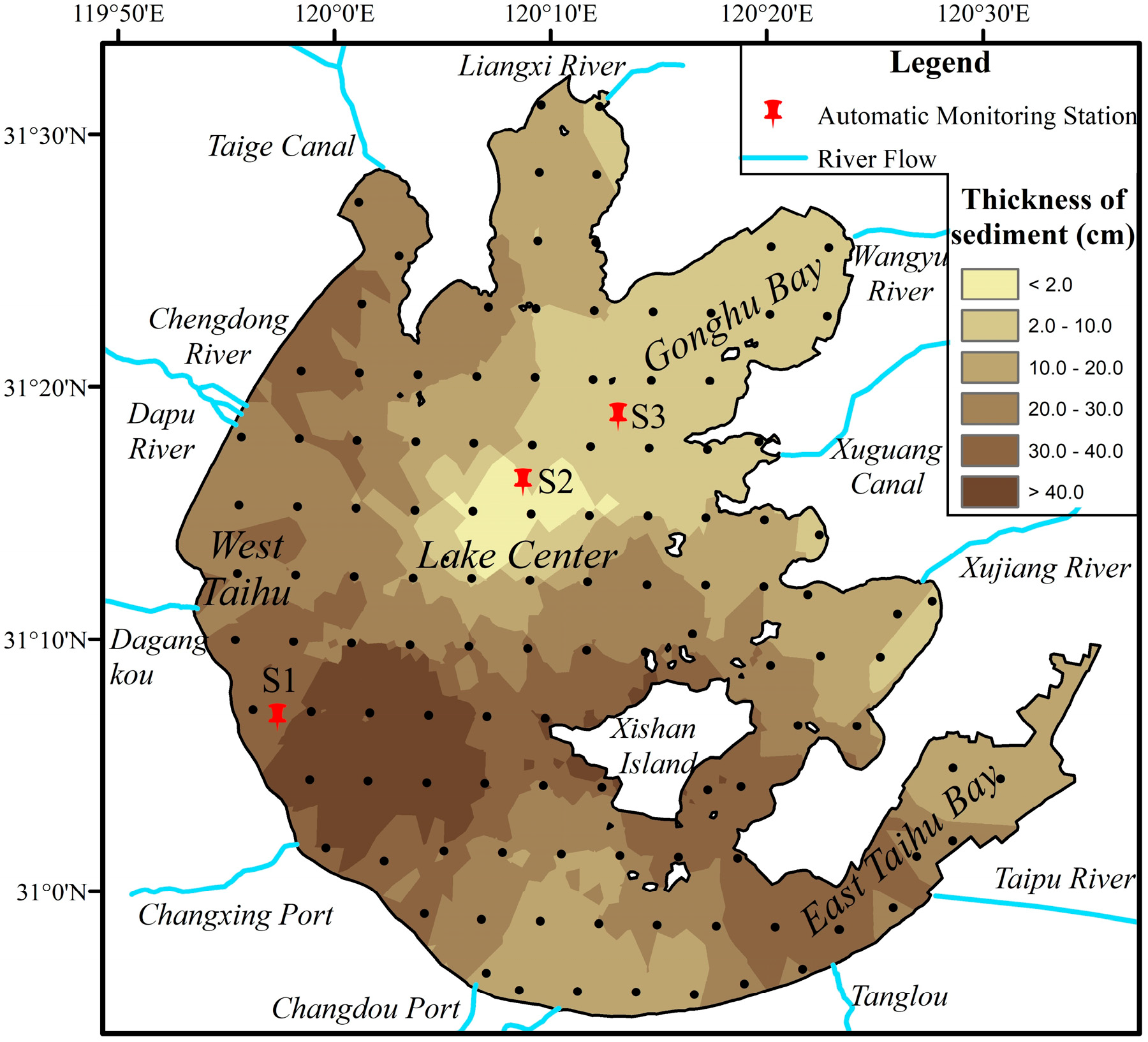
3.1. Sediment Characteristics

Most of the sediments are located in the western and southern parts of the lake; and the sediment thickness is relatively higher (lower) in the southwestern (northeastern) lake; few sediments are located at Station Lake Center (S2) (Figure 3).

At S1, S2, and S3, the sludge thickness was 20, 0 (no sludge), and 7.5 cm, respectively; the density of the bed sediments was 1.58, 1.90, and 1.62 kg m⁻³; the moisture content was 53.82%, 45.45%, 51.93%; the critical shear stress was 0.029, 0.055, and 0.032 N m⁻².

3.2. Turbidity, Wind, and Chl-a during In Situ Observations

During the period of in situ observations, the mean turbidity at S1, S2, and S3 was 116.46, 60.51, and 45.15 NTU, respectively (

Table 2. Statistical characteristics of turbidity, wind speed, and chlorophyll-a (Chl-a).

		S1	S2	S3
Turbidity (NTU)	Mean	116.46	60.51	45.15
	Standard Deviation	80.39	36.92	37.84
	Maximum	314.20	289.30	259.40
Wind Speed (m s−1)	Mean	4.27	4.75	4.29
	Standard Deviation	2.30	2.36	2.62
	Maximum	12.26	14.97	19.00
Chl-a (mg m−3)	Mean	23.27	14.62	30.80
	Standard Deviation	15.46	9.03	26.60
	Maximum	59.99	33.59	105.35

), and the mean Chl-a concentration at S1, S2, and S3 was 23.27, 14.62, 30.80 ug L⁻¹, respectively. Meanwhile, the mean wind speed at S1, S2, and S3 was 4.27, 4.75, and 4.29 m s⁻¹, respectively (Table 2); the wind speed evidently affects the turbidity.

The Pearson correlation analysis method could be used to select the influencing factors of the predicted variable [31,32]. Therefore, we calculated the Pearson correlation coefficients between the different environmental variables measured at S2. As shown in Figure 4, the turbidity is positively (negatively) correlated with Chl-a, pressure, and wind speed (temperature). The correlation coefficient between the wind speed and turbidity was the largest (r = 0.57, p < 0.05). Global studies have shown [33,34,35] that wind is the main driving force of sediment resuspension in shallow lakes. Therefore, we developed the LSTM-based turbidity model using synchronous wind speed.

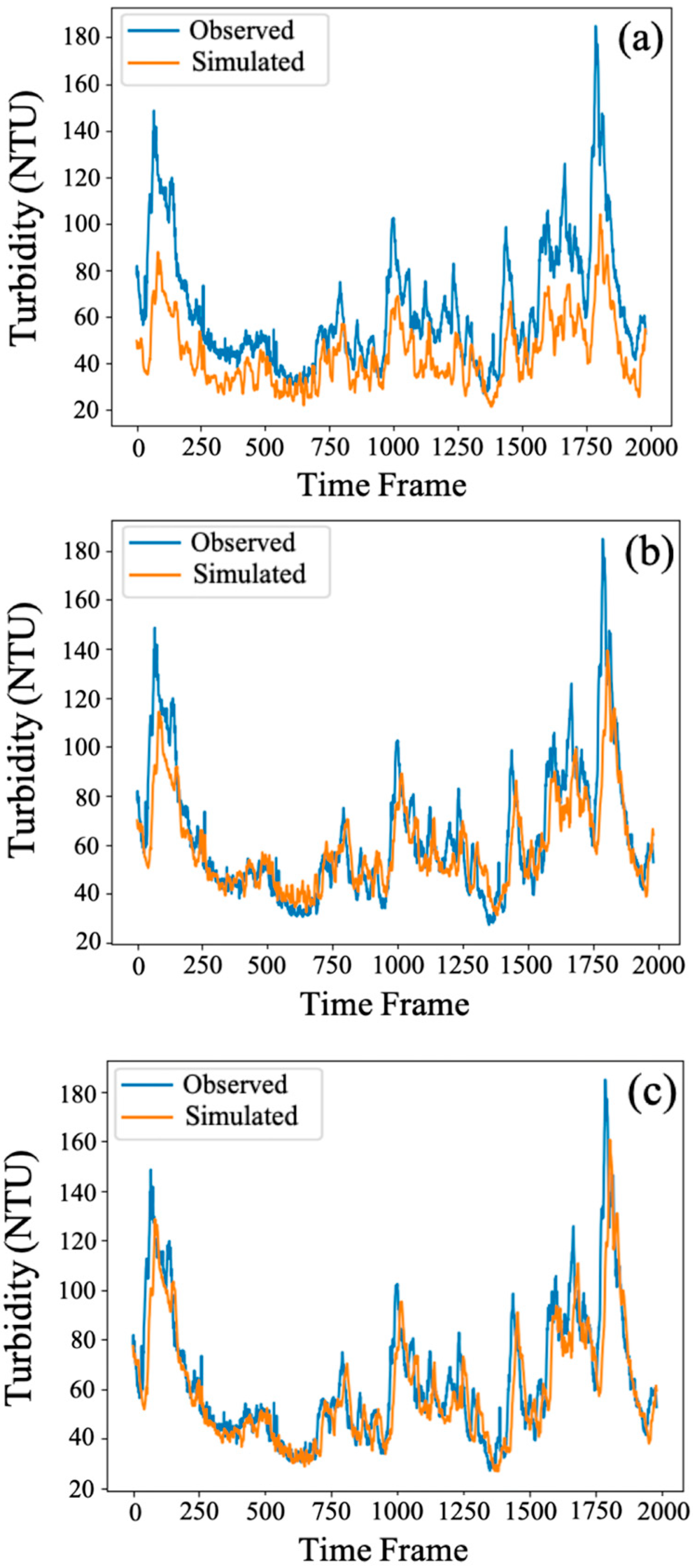
3.3. Evaluation of LSTM Model Accuracy

The turbidity time series from S2 were used to train the LSTM-based turbidity model. The results showed that the model error increased with the forecast period (Figure 5). The NSE value was >0.9 and the RMSE value was <10 NTU when the forecast period was 2 h. When the forecast period exceeded 10 h, the NSE value decreased to <0.5 and the RMSE value increased to >20 NTU. However, the input time window had no influence on the model prediction. Therefore, to minimize the demand on computing resources, the input time window was set to 2 h.

The size of the training set could influence the predictions of the LSTM-based turbidity model (Figure 6). When the size of the training set increased from 600 to 3000 sets, the NSE value of the prediction increased from 0.1 to nearly 0.7, and the RMSE value reduced by more than 10 NTU. When the size of the training set increased to 9000 sets, the RMSE and NSE values of the prediction became <13 NTU and >0.9, respectively.

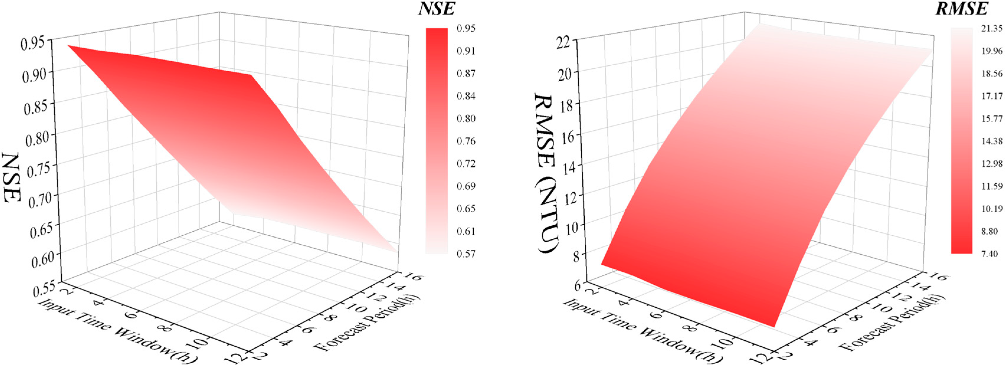
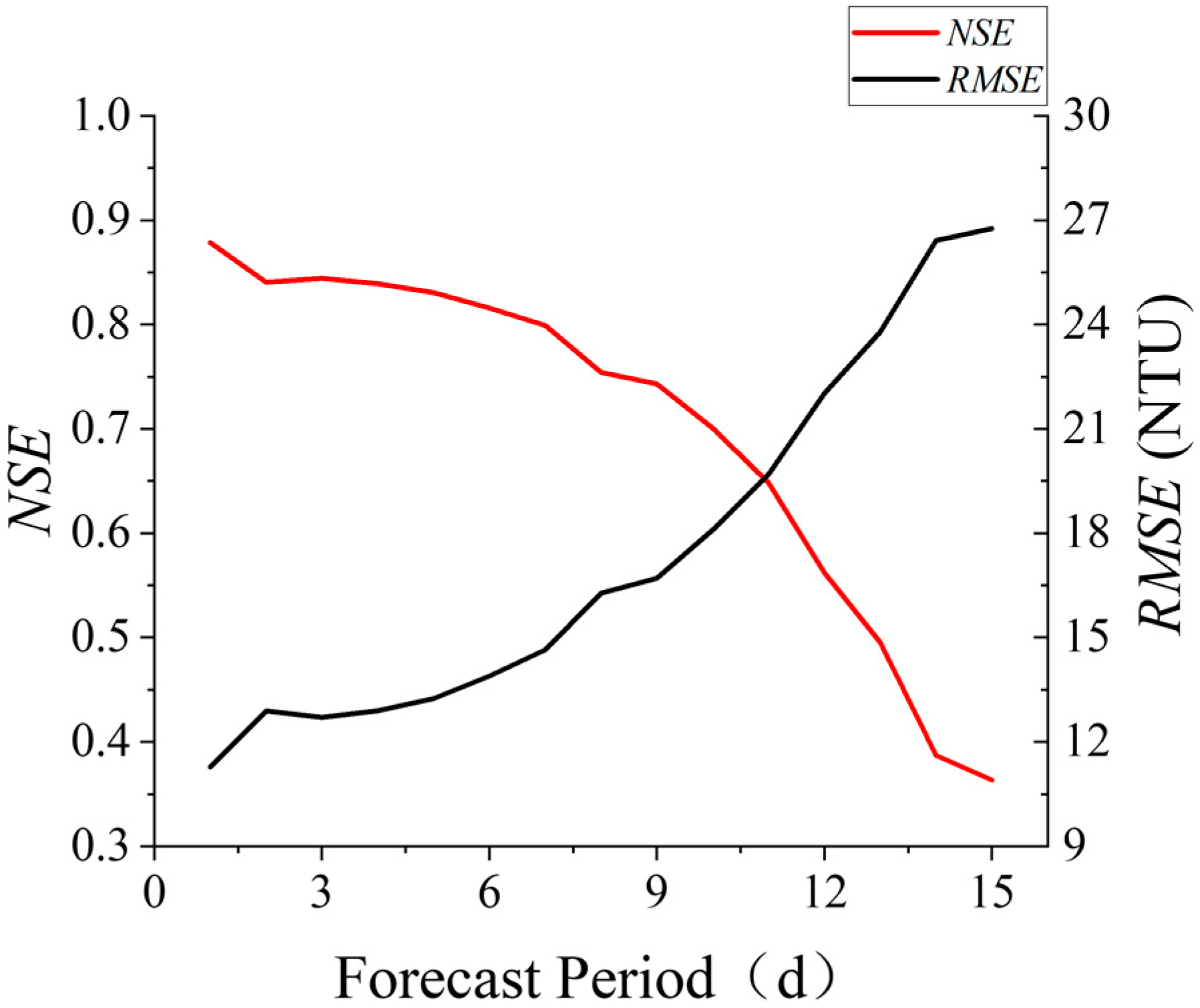
3.4. Model Experiments

3.4.1. LSTM_W Scenario

Figure 5 shows the NSE and RMSE values of the LSTM_S2-W1 Scenario, the NSE value decreased and the RMSE value increased with increasing forecast period; the NSE value was below 0.5 and the RMSE value was above 20 NTU at a forecast period of 10 h. However, for LSTM_S2-W2, the RMSE value increased with the forecast period, and reached 20 NTU at a forecast period of 12 days (Figure 7); the NSE value decreased with the forecast period and reached 0.7 at a forecast period of nine days; the rate of the decrease in the NSE value increased considerably for the forecast periods of >12 days.

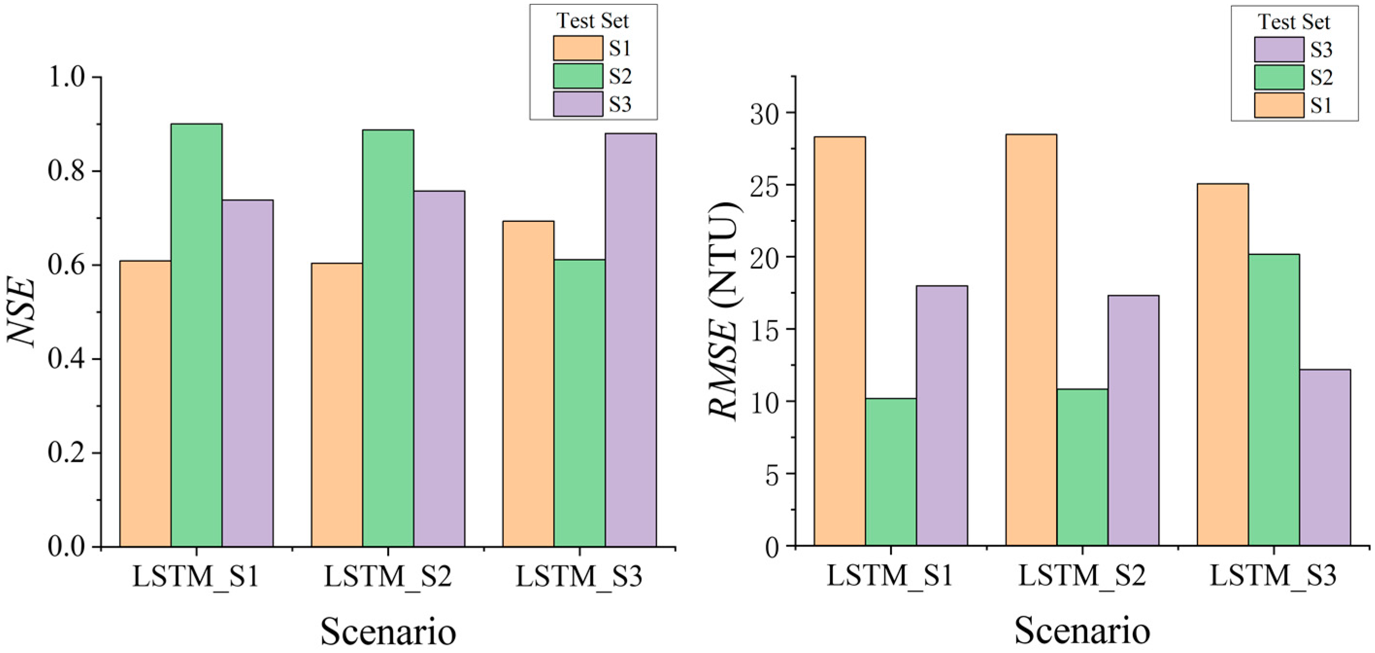
3.4.2. LSTM_S Scenario

Figure 8 shows the results of the LSTM_S Scenario; the NSE values of all the predictions were >0.6. The performance of LSTM_S1 was similar to that of LSTM_S2. Among the 3 scenarios, the LSTM_S2 performed the best, with a NSE of 0.90 and RMSE of 10.20 NTU. Meanwhile, LSTM_S1 performed the poorest with a NSE of 0.60 and RMSE of 28.30 NTU.

The NSE (RMSE) produced by LSTM_S31, S32, and S33, was 0.69 (25.06NTU), 0.61 (20.19NTU) and 0.88 (12.19 NTU), respectively. We compared the performance of LSTM_S3 with the performance of LSTM_S1 and that of LSTM_S2. For LSTM_S3, the performance at S2 was the poorest.

4. Discussion

We developed LSTM-based turbidity models using high-frequency time series data obtained from stations S1, S2, and S3. We found that increasing the size of the training set considerably improved the prediction accuracy, while the input time window had almost no impact on the prediction results.

Wind waves and lake currents are two hydrodynamic processes that influence the turbidity in large shallow lakes [36]. In Lake Taihu, wind waves are the dominant mechanism of sediment erosion and resuspension [37,38]; resuspended sediments are horizontally transported by the lake currents. These processes determine the spatial distribution of turbidity in Lake Taihu. Compared to the model that did not consider the future wind speed, the effective forecast period of the model considering the future wind speed increased to 12d when the criterion of NSE > 0.5 was employed to define the availability of the machine-learning-based model [39]. When the forecast period was <24 h, the RMSE produced by the LSTM-based turbidity model was <15 NTU, while the NSE was >0.8. However, under the same conditions, the RMSE and NSE produced by the regression-analysis-based turbidity models were >20 NTU and <0.5, respectively.

In addition to wind, ecological variables (e.g., sediment properties and algal biomass) [11] also influence turbidity. We collected and analyzed the bed sediments at stations S1, S2, and S3. The sediment thickness at S2 was the lowest and the critical shear stress was the highest (0.055 N m⁻²) among the three sites (Figure 3); this indicates that the likelihood of sediment erosion was the lowest at site S2, where the low Chl-a concentration and relatively constant wind fetch amplified the influence of the wind on the turbidity. Therefore, we inferred that wind was the major factor influencing turbidity at the Lake Center. At site S3, the sediment thickness was 7.5 cm, and the critical shear stress was 0.032 N m⁻², indicating that the sediments could be easily eroded and resuspended to increase turbidity. The Chl-a concentration was significantly higher at site S3 than at site S2 (p < 0.05); therefore, the wind, sediment properties, and Chl-a jointly influenced the turbidity at site S3. As a result, the LSTM_S2 and LSTM_S3 fully learned the turbidity changes caused by wind and by the joint influence of the ecological variables, respectively. Thus, LSTM_S2 (LSTM_S3) accurately predicted the turbidity at site S2 (S3), with a NSE of 0.89 and a RMSE of 10.84 NTU (a NSE of 0.88 and a RMSE of 12.19 NTU). However, the accuracy of the turbidity predictions at the other sites was lower because of the spatial heterogeneity in the environmental factors.

The environment at site S1 was similar to that at site S3. The bed sediments could resuspend easily (with a thickness of 20 cm and a critical shear stress of only 0.029 N m⁻²) and the Chl-a concentration was relatively high (23.27 mg m⁻³). The LSTM_S1 and LSTM_S2 at all of the three sites showed comparable performances. Considering the great performance of LSTM_S2 and LSTM_S3, LSTM_S1 could theoretically learn the turbidity changes caused by the factors above. However, neither LSTM_S1 nor the other two models could predict the turbidity at site S1 with a relative high accuracy; the performance of LSTM_S1 was lower at site S1 than at sites S2 and S3. This could be explained by the complex hydrodynamic processes (e.g., inflow, wind setup, wave breaking, and alongshore currents) occurring at site S1 [40,41], which was near the shore of West Taihu. The complex hydrodynamic processes complicated the turbidity changes and weakened the learning of the LSTM from the time series data, and subsequently decreased the accuracy of the LSTM-based turbidity model.

Although the Chl-a concentration, sediment properties and other environmental factors would influence the turbidity in Lake Taihu, wind played a key role. Therefore, the model trained with the wind speed and turbidity time series from any a given zone of Lake Taihu could predict the turbidity in other zones with a relatively high accuracy (NSE > 0.6). However, we recommend establishing monitoring stations in zones where turbidity is influenced by fewer environmental factors to increase model universality; the length of the time series data and the diversity of the input variables should be increased to improve the model performance.

5. Conclusions

We developed LSTM-based models for three zones in Lake Taihu and the comparison between them showed that the lake environment influences the model performance in two ways. On one hand, the spatial heterogeneity of the Chl-a concentrations and sediment physicochemical properties lowers the applicability of the point-based models to other zones in the lake. On the other hand, the complex hydrodynamics weaken the learning of LSTM from the turbidity time series in the training phase and reduce the model accuracy. Overall, although the prediction accuracy would fluctuate, the model developed based on the observed data from any station could predict the turbidity changes in other zones with a relatively high accuracy (NSE > 0.6).

References

1. Abdul-Wahab, S.A.; Al-Alawi, S.M. Assessment and prediction of tropospheric ozone concentration levels using artificial neural networks. Environ. Model. Softw. 2002, 17, 219–228. [Google Scholar] [CrossRef]
2. Bailey, M.C.; Hamilton, D.P. Wind induced sediment resuspension: A lake-wide model. Ecol. Model. 1997, 99, 217–228. [Google Scholar] [CrossRef]
3. Bartram, J. Water Quality Monitoring: A Practical Guide to the Design and Implementation of Freshwater Quality Studies and Monitoring Programmes; CRC Press: London, UK, 1996; 365p. [Google Scholar]
4. Barzegar, R.; Aalami, M.T.; Adamowski, J. Short-term water quality variable prediction using a hybrid CNN-LSTM deep learning model. Stoch. Environ. Res. Risk Assess. 2020, 34, 415–433. [Google Scholar] [CrossRef]
5. Basodi, S.; Ji, C.; Zhang, H.; Pan, Y. Gradient amplification: An efficient way to train deep neural networks. Big Data Min. Anal. 2020, 3, 196–207. [Google Scholar] [CrossRef]
6. Bengtsson, L.; Hellstrom, T. Wind-induced resuspension in a small shallow lake. Hydrobiologia 1992, 241, 163–172. [Google Scholar] [CrossRef]
7. Chen, N.; Mao, S.; Li, D.; Yue, J. PM2.5 prediction model based on multi-station co-training neural network. Sci. Surv. Mapp. 2018, 43, 87–93. [Google Scholar]
8. Chen, Y.; Cheng, Q.; Fang, X.; Yu, H.; Li, D. Principal component analysis and long short-term memory neural network for predicting dissolved oxygen in water for aquaculture. Trans. Chin. Soc. Agric. Eng. 2018, 34, 183–191. [Google Scholar]
9. Ding, W.; Wu, T.; Qin, B.; Lin, Y.; Wang, H. Features and impacts of currents and waves on sediment resuspension in a large shallow lake in China. Environ. Sci. Pollut. Res. 2018, 25, 36341–36354. [Google Scholar] [CrossRef]
10. Ding, W.; Zhao, J.; Qin, B.; Wu, T.; Zhu, S.; Li, Y.; Xu, S.; Ruan, S.; Wang, Y. Exploring and quantifying the relationship between instantaneous wind speed and turbidity in a large shallow lake: Case study of Lake Taihu in China. Environ. Sci. Pollut. Res. 2021, 28, 16616–16632. [Google Scholar] [CrossRef]
11. Figueroa-Pico, J.; Carpio, A.J.; Tortosa, F.S. Turbidity: A key factor in the estimation of fish species richness and abundance in the rocky reefs of Ecuador. Ecol. Indic. 2020, 111, 106021. [Google Scholar] [CrossRef]
12. Gers, F.A.; Schmidhuber, J.; Cummins, F. Learning to Forget: Continual Prediction with LSTM. Neural Comput. 2000, 12, 2451–2471. [Google Scholar] [CrossRef] [PubMed]
13. Guo, Y.; Lai, X. Water level prediction of Lake Poyang based on long short-term memory neural network. J. Lake Sci. 2020, 32, 865–876. [Google Scholar] [CrossRef]
14. Hochreiter, S.; Schmidhuber, J. Long Short-Term Memory. Neural Comput. 1997, 9, 1735–1780. [Google Scholar] [CrossRef] [PubMed]
15. Hu, K.; Wang, S.; Pang, Y. Suspension-sedimentation of sediment and release amount of internal load in Lake Taihu. J. Lake Sci. 2014, 26, 191–199. [Google Scholar] [CrossRef] [Green Version]
16. Iglesias, C.; Martínez Torres, J.; García Nieto, P.J.; Alonso Fernández, J.R.; Díaz Muñiz, C.; Piñeiro, J.I.; Taboada, J. Turbidity Prediction in a River Basin by Using Artificial Neural Networks: A Case Study in Northern Spain. Water Resour. Manag. 2013, 28, 319–331. [Google Scholar] [CrossRef]
17. Jalil, A.; Li, Y.; Zhang, K.; Gao, X.; Wang, W.; Khan, H.O.S.; Pan, B.; Ali, S.; Acharya, K. Wind-induced hydrodynamic changes impact on sediment resuspension for large, shallow Lake Taihu, China. Int. J. Sediment Res. 2019, 34, 205–215. [Google Scholar] [CrossRef]
18. Fanxiang, K.; Ronghua, M.; Junfeng, G.; Xiaodong, W. The theory and practice of prevention, forecast and warning on cyanobacteria bloom in Lake Taihu. Sci. Limnol. Sin. 2009, 21, 314–328. [Google Scholar] [CrossRef] [Green Version]
19. Kumar, D.N.; Raju, K.S.; Sathish, T. River Flow Forecasting using Recurrent Neural Networks. Water Resour. Manag. 2004, 18, 143–161. [Google Scholar] [CrossRef]
20. Lesht, B.M. Relationship between sediment resuspension and the statistical frequency-distribution of bottom shear-stress. Mar. Geol. 1979, 32, M19–M27. [Google Scholar] [CrossRef]
21. Luo, L.; Qin, B.; Hu, W.; Zhang, F. Wave characteristics in Lake Taihu. J. Hydrodyn. 2004, 19, 664–670. [Google Scholar]
22. Luo, L.C.; Qin, B.Q.; Zhu, G.W. Sediment distribution pattern mapped from the combination of objective analysis and geostatistics in the large shallow Tatihu Lake, China. J. Environ. Sci. 2004, 16, 908–911. [Google Scholar]
23. Mallet, D.; Pelletier, D. Underwater video techniques for observing coastal marine biodiversity: A review of sixty years of publications (1952–2012). Fish. Res. 2014, 154, 44–62. [Google Scholar] [CrossRef] [Green Version]
24. Gaffar, A.F.O.; Puspitasari, N. Water Level Prediction of Lake Cascade Mahakam Using Adaptive Neural Network Backpropagation (ANNBP). IOP Conf. Ser. Earth Environ. Sci. 2018, 144, 012009. [Google Scholar]
25. Palani, S.; Liong, S.Y.; Tkalich, P. An ANN application for water quality forecasting. Mar. Pollut. Bull. 2008, 56, 1586–1597. [Google Scholar] [CrossRef]
26. Pang, Y.; Li, Y.P.; Luo, L.C. Study on the simulation of transparency of Lake Taihu under different hydrodynamic conditions. Sci. China Earth Sci. 2006, 49, 162–175. [Google Scholar] [CrossRef]
27. Qin, B.; Xu, P.; Wu, Q.; Luo, L.; Zhang, Y. Environmental issues of Lake Taihu, China. Hydrobiologia 2007, 581, 3–14. [Google Scholar] [CrossRef]
28. Rajaee, T. Wavelet and ANN combination model for prediction of daily suspended sediment load in rivers. Sci. Total Environ. 2011, 409, 2917–2928. [Google Scholar] [CrossRef]
29. Sengorur, B.; Dogan, E.; Koklu, R.; Samandar, A. Dissolved oxygen estimation using artificial neural network for water quality control. Fresenius Environ. Bull. 2006, 15, 1064–1067. [Google Scholar]
30. Shi, M.; Xu, K.; Wang, J.; Yin, R.; Wang, T.; Yong, T. Short-Term Photovoltaic Power Forecast Based on Long Short-Term Memory Network. In Proceedings of the 2019 IEEE 3rd International Electrical and Energy Conference (CIEEC), Beijing, China, 7–9 September 2019; pp. 2110–2116. [Google Scholar]
31. Song, C.; Zhang, H. Study on turbidity prediction method of reservoirs based on long short term memory neural network. Ecol. Model. 2020, 432, 109–210. [Google Scholar] [CrossRef]
32. Valipour, R.; Boegman, L.; Bouffard, D.; Rao, Y.R. Sediment resuspension mechanisms and their contributions to high-turbidity events in a large lake. Limnol. Oceanogr. 2017, 62, 1045–1065. [Google Scholar] [CrossRef] [Green Version]
33. Wu, T.; Qin, B.; Huang, A.; Sheng, Y.; Feng, S.; Casenave, C. Reconsideration of wind stress, wind waves, and turbulence in simulating wind-driven currents of shallow lakes in the Wave and Current Coupled Model (WCCM) version 1.0. Geosci. Model Dev. 2022, 15, 745–769. [Google Scholar] [CrossRef]
34. Wu, T.-F.; Qin, B.-Q.; Zhu, G.-W.; Zhu, M.-Y.; Li, W.; Luan, C.-M. Modeling of turbidity dynamics caused by wind-induced waves and current in the Taihu Lake. Int. J. Sediment Res. 2013, 28, 139–148. [Google Scholar] [CrossRef]
35. Xu, G.; Xia, L. Short-Term Prediction of Wind Power Based on Adaptive LSTM. In Proceedings of the 2018 2nd IEEE Conference on Energy Internet and Energy System Integration (EI2), Beijing, China, 20–22 October 2018. [Google Scholar]
36. Yoon, H.-S. Time Series Data Analysis using WaveNet and Walk Forward Validation. J. Korea Soc. Simul. 2021, 30, 1–8. [Google Scholar] [CrossRef]
37. Yu, Z.; Yang, K.; Luo, Y.; Shang, C. Spatial-temporal process simulation and prediction of chlorophyll-a concentration in Dianchi Lake based on wavelet analysis and long-short term memory network. J. Hydrol. 2020, 582, 124488. [Google Scholar] [CrossRef]
38. Zhang, B.; Zou, G.; Qin, D.; Lu, Y.; Jin, Y.; Wang, H. A novel Encoder-Decoder model based on read-first LSTM for air pollutant prediction. Sci. Total Environ. 2021, 765, 144507. [Google Scholar] [CrossRef] [PubMed]
39. Zhang, Y.; Qin, B.; Chen, W. A study on total suspended matter in lake taihu. Resour. Environ. Yangtze Basin 2004, 13, 266–271. [Google Scholar]
40. Zhang, Y.; Yao, X.; Wu, Q.; Huang, Y.; Zhou, Z.; Yang, J.; Liu, X. Turbidity prediction of lake-type raw water using random forest model based on meteorological data: A case study of Tai lake, China. J. Environ. Manag. 2021, 290, 112657. [Google Scholar] [CrossRef]
41. Zheng, S.-S.; Wang, P.-F.; Wang, C.; Hou, J. Sediment resuspension under action of wind in Taihu Lake, China. Int. J. Sediment Res. 2015, 30, 48–62. [Google Scholar] [CrossRef]
Figure 1. Lake Taihu and locations of monitoring stations, Taihu Laboratory for Lake Ecosystem Research chlorophyll-a sampling sites, inflows, outflows, and sediment sampling sites.
Water 15 00387 g001
Figure 2. Flow chart of LSTM-based turbidity model development.
Water 15 00387 g002
Figure 3. Spatial distribution of sediments in Lake Taihu.
Water 15 00387 g003
Figure 4. Pearson’s correlation coefficients between different environmental variables measured at S2.
Water 15 00387 g004
Figure 5. (Left) NSE and (right) RMSE of S2-data-based LSTM model with different input time windows and forecast periods without future wind speed as an additional input variable.
Water 15 00387 g005
Figure 6. Observed and simulated turbidity based on data collected at S2. Simulated turbidity using different sizes of training set: (a) 600, (b) 3000, and (c) 9000 sets.
Water 15 00387 g006
Figure 7. NSE and RMSE of the LSTM model with future wind speed as an additional input variable.
Water 15 00387 g007
Figure 8. (Left) NSE and (right) RMSE of the LSTM model with different training and testing data.
Water 15 00387 g008