Article

Groundwater Sustainability Assessment against the Population Growth Modelling in Bima City, Indonesia

by
Abdullah Husna
1,
Rizka Akmalia
2,
Faizal Immaddudin Wira Rohmat
3,4,*,
Fauzan Ikhlas Wira Rohmat
4,
Dede Rohmat
5,
Winda Wijayasari
4,
Pascalia Vinca Alvando
4 and
Arif Wijaya
6
1
Geological Agency of Indonesia, Ministry of Energy and Mineral Resources, Jalan Diponegoro No. 57, Cihaur Geulis, Kec. Cibeunying Kaler, Bandung 40122, West Java, Indonesia
2
Deltares Indonesia, Wisma Iskandarsyah A-10 Suite 3&4, Jalan Iskandarsyah Raya Kavling 12-14, South Jakarta 12160, Jakarta, Indonesia
3
Department of Water Resources Engineering and Management, Faculty of Civil and Environmental Engineering, Bandung Institute of Technology, Jatinangor Campus, Bandung 45363, West Java, Indonesia
4
Water Resources Development Center, Bandung Institute of Technology, CIBE Building 5th Floor, Jalan Ganesa No. 10, Bandung 40132, West Java, Indonesia
5
Department of Geography, Indonesia University of Education, Jalan Dr. Setiabudhi No. 229, Bandung 40154, West Java, Indonesia
6
Mining Engineering Department, Muhammadiyah University of Mataram, KH. Ahmad Dahlan Street No. 1, Pagesangan, Mataram 83115, West Nusa Tenggara, Indonesia
*
Author to whom correspondence should be addressed.
Water 2023, 15(24), 4262; https://doi.org/10.3390/w15244262
Submission received: 11 October 2023 / Revised: 9 December 2023 / Accepted: 10 December 2023 / Published: 13 December 2023

Abstract

:
Most of Indonesia’s population lives in areas with volcanic–alluvium geological characteristics. Based on the national hydrogeological map of the Indonesian Geological Agency, areas with volcanic–alluvium geological conditions have high groundwater potential and potential for groundwater damage. This study aims to test the resilience of groundwater areas with volcanic–alluvial characteristics to population growth. The MODFLOW groundwater model was built based on the site’s volcanic and alluvial geological conditions. This groundwater model was tested against pumping scenarios based on population water demand in 2011–2020 and then predicted population growth until 2030. The result shows that groundwater resilience in volcanic–alluvium locations has different characteristics based on lithology and population density characteristics. Urban areas that are mostly located in alluvium areas tend to have a linear groundwater decline pattern but have the sharpest groundwater decline gradient. In contrast, suburban areas in the alluvium-to-volcanic transition area initially experience exponential groundwater decline but change to linear, while rural areas located in volcanic areas that become the main development target have exponential groundwater decline characteristics. To counteract the continuous depletion of groundwater, researchers conducted a scenario for optimizing surface water use. Based on the results of the scenario, a 60% reduction in groundwater use is sufficient to stop continuous groundwater depletion. The results of this study can be used as a recommendation for long-term water resources management targets for volcanic and alluvium areas that are being targeted for development.

1. Introduction

Groundwater is a major source of freshwater resources humans utilize for domestic, agricultural, industrial, and other purposes [1,2]. Groundwater plays a critical role in human activities, as it is the largest unfrozen freshwater resource on the planet. Globally, approximately one-third of the global population depends on groundwater as the primary source of drinking water [2]. Groundwater is essential for survival in unstable or scarce surface water sources. Groundwater is used not only for drinking but also for domestic uses like washing, cooking, and hygiene, which directly impacts the health and living standards in countless communities. Groundwater supplies are also crucial to many industries, including manufacturing and agriculture. The largest groundwater consumer is agriculture, with irrigation systems in many areas heavily reliant on underground resources. This reliance ensures harvests even in unfavorable climatic conditions, providing food security for millions of people. Furthermore, groundwater availability and quality are closely related to industries like real estate, tourism, and, in some cases, energy production. Thus, a steady groundwater supply promotes employment, spurs economic expansion, and increases the capacity of local economies to withstand environmental and climatic variabilities.
With population growth, industrial development, and climate variability, the stress on groundwater pressure is mounting. Groundwater sources are threatened by overexploitation, contamination, and improperly planned development. Such a problem is more pronounced in areas where conjunctive surface–groundwater use is present and the surface water sources are stressed. For example, in the region where surface water is polluted [2,3], the demand for water is growing [4,5], water-intensive agriculture activities exist [6,7,8,9], and resilient surface water pipeline services are unavailable in urbanized areas [10,11,12]. As human population growth is still producing a positive trend, while resilient surface water services require planning and investments, regions with unfulfilled water demands will still rely on groundwater sources [11]. Such a situation will make groundwater sustainability a pressing matter, thus requiring careful study and long-term planning.
Given the realities mentioned above, it is important to protect the availability of groundwater sources. Groundwater, being a dynamic and finite resource, requires careful management considering perturbation factors, especially those related to anthropogenic activities. Understanding the system and long-term sustainability is paramount, especially in places where the population continuously grows while dependent on groundwater resources. This study uses the example case of Bima City and the associated Rontu Watershed (Figure 1), where groundwater use is essential in daily human activities in this semi-arid area. This work presents the use of a spatial population growth model to predict long-term groundwater demand using a MODFLOW groundwater numerical model. It is crucial to place this study within a larger, global context as the takeaways from this research may have particular applicability, especially for areas where groundwater sources are essential and the population is continuously growing. This research contributes to the understanding and improvement of solutions for groundwater sustainability, especially in semi-arid developing communities that rely on groundwater sources.

2. Materials and Methods
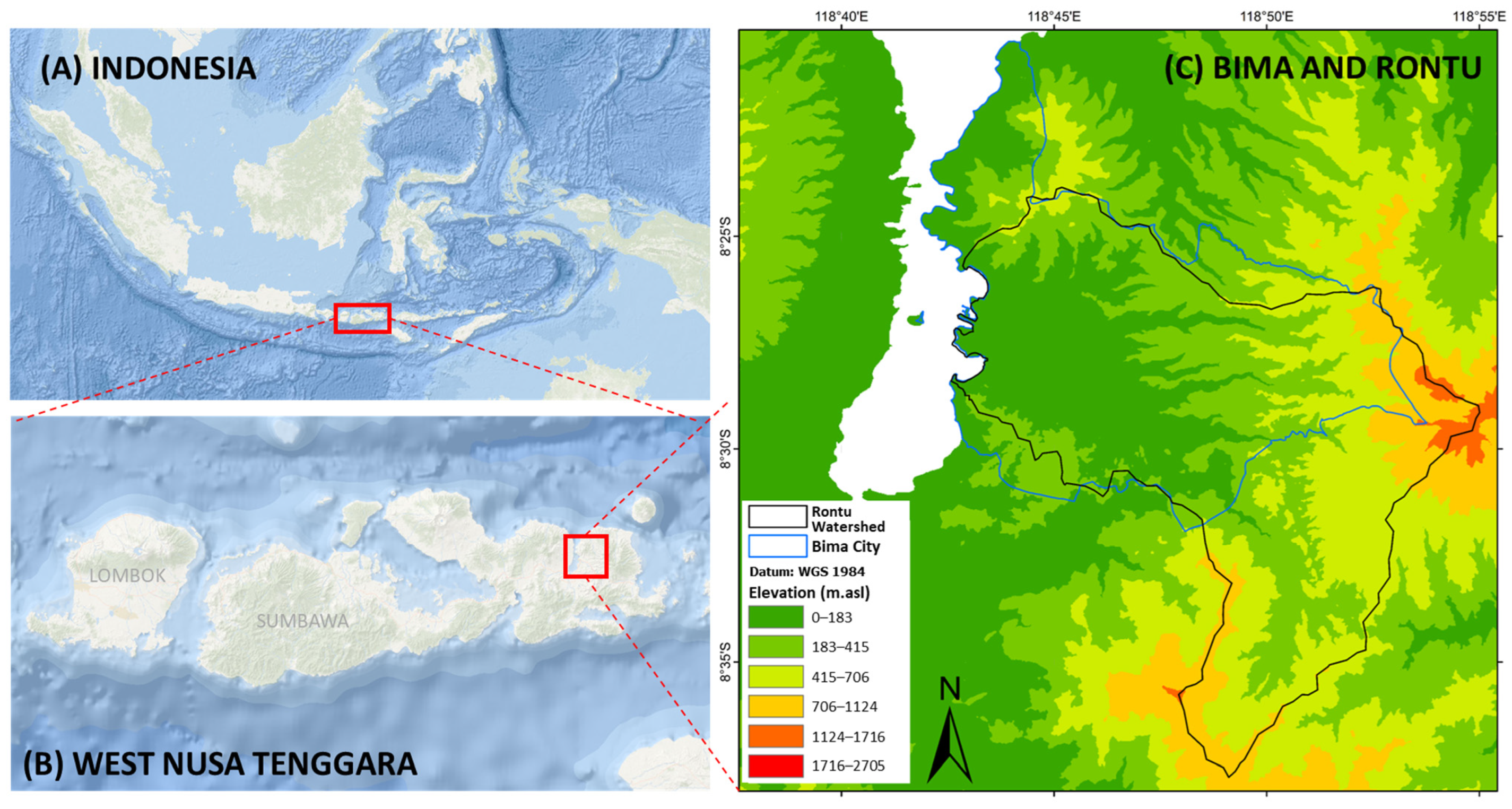
2.1. Study Domain

Indonesia is an archipelago formed on a subduction zone where most islands are composed of volcanic rocks in highland areas and alluvium in coastal areas [13]. Most cities and settlements in Indonesia are concentrated in coastal areas. Indonesia is a tropical region with average rainfall above 1500 mm/year [14], resulting in high groundwater potential on average. Since Indonesia is the world’s fourth-most populous country and most of Indonesia’s population prioritizes groundwater as the main water source [15], groundwater stress in these areas is high. Some locations with high groundwater potential now have permanent groundwater damage due to excessive groundwater withdrawal, such as in the Jakarta Basin and Semarang-Demak Basin, where groundwater potential cannot keep up with development, causing land subsidence and saltwater intrusion [16,17].
This research was conducted in a location with a growing population in a semi-arid area with volcanic–alluvium geological conditions in Indonesia, i.e., the Rontu Watershed, which includes Bima City and its surroundings. The location is in the southeast part of the Indonesian archipelago, administratively in the province of West Nusa Tenggara (Figure 1). Bima is a developing city where the population initially increased along with the development of mining practices in the area. As for the land use and land cover in the Rontu Watershed, the area is predominantly 148 km2 of barren land followed by 67 km2 of natural vegetation. The built-up area covers 26 km2 of the total study area. Geographically, Bima is similar to most developing regions in Indonesia, where the growing city starts from a small population community dominated by just a handful of occupations. The city is situated in an alluvium–volcanic area with intermittent streams and groundwater as its main water source. The city then continually grows over time into a larger community and more diverse occupations, which Bima City and other cities in Indonesia are currently experiencing.

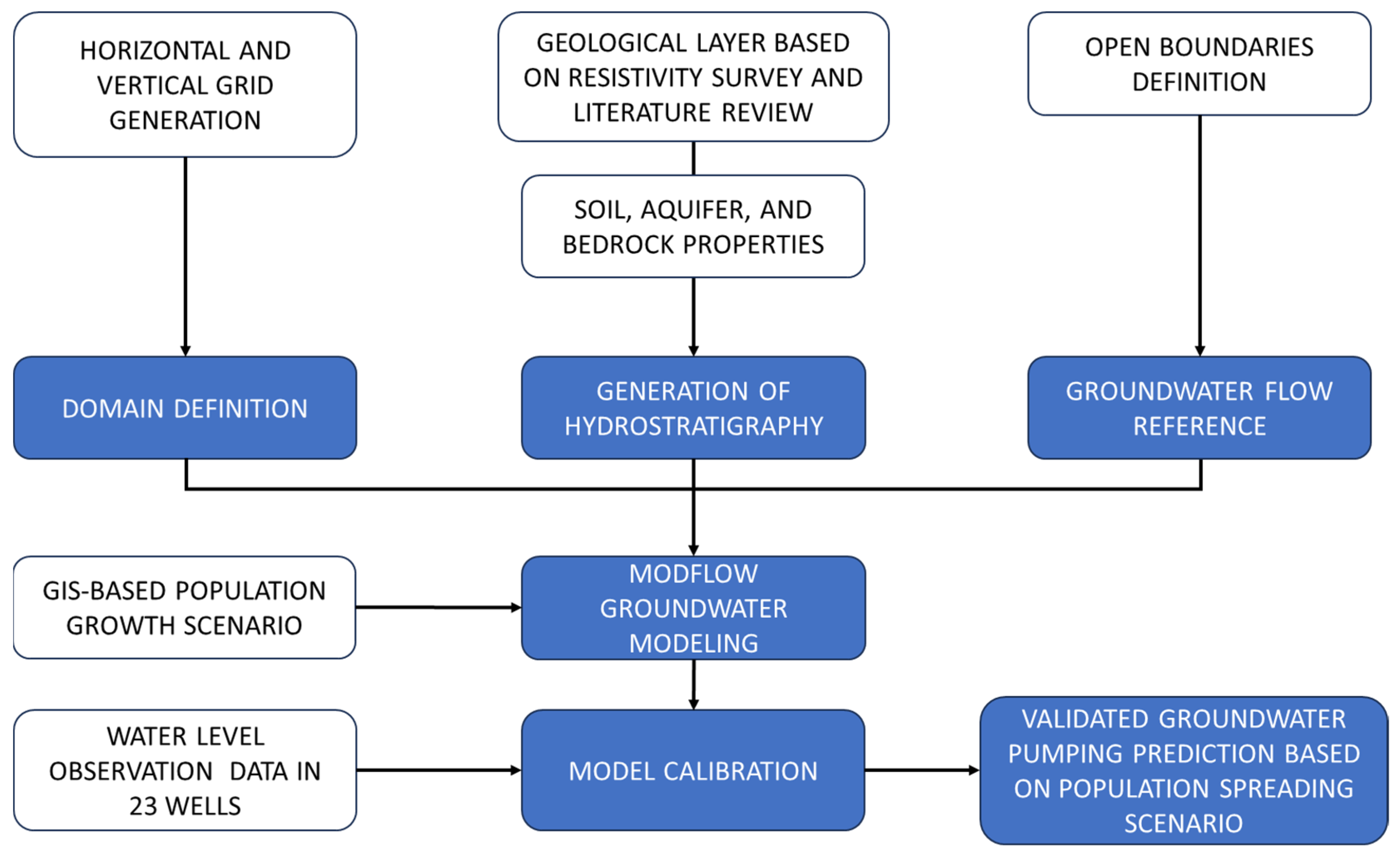
2.2. General Methodology

This research evaluates the impact of the population growth of Bima City on groundwater availability through modeling, especially in the amount of pumping in the region. The general flowchart of the study is presented in Figure 2. The modeling started with a domain definition, i.e., the boundaries of the model and the horizontal and vertical grid generation. The modeling was then continued by inputting the geological or hydrostratigraphy layers based on secondary and primarily collected datasets. The primary datasets include field-surveyed hydraulic conductivity data and well-depth data for model calibration. The groundwater modeling used the MODFLOW model with the aid of ModelMuse GUI for conceptualization, data input, and execution [18]. Other secondary datasets involved were the geological map dataset from the Geological Agency of the Republic of Indonesia and population density sourced from Statistics Indonesia (Badan Pusat Statistik, henceforth BPS). These two datasets were used for data cross-checking.
This research can be a reference for water management that considers climate, population, and hydrogeological conditions. An effective and efficient groundwater management strategy can be built according to an area’s geological conditions and population density. This is important because every city has different geological and population density conditions. Also, since the secondary data are all available throughout Indonesia, this method is applicable nationwide. This applicability especially applies to groundwater studies that are based on secondary geological and population density data. For a more detailed study, taking on primary data such as the groundwater level and information from geoelectric surveys is suggested to calibrate the model.

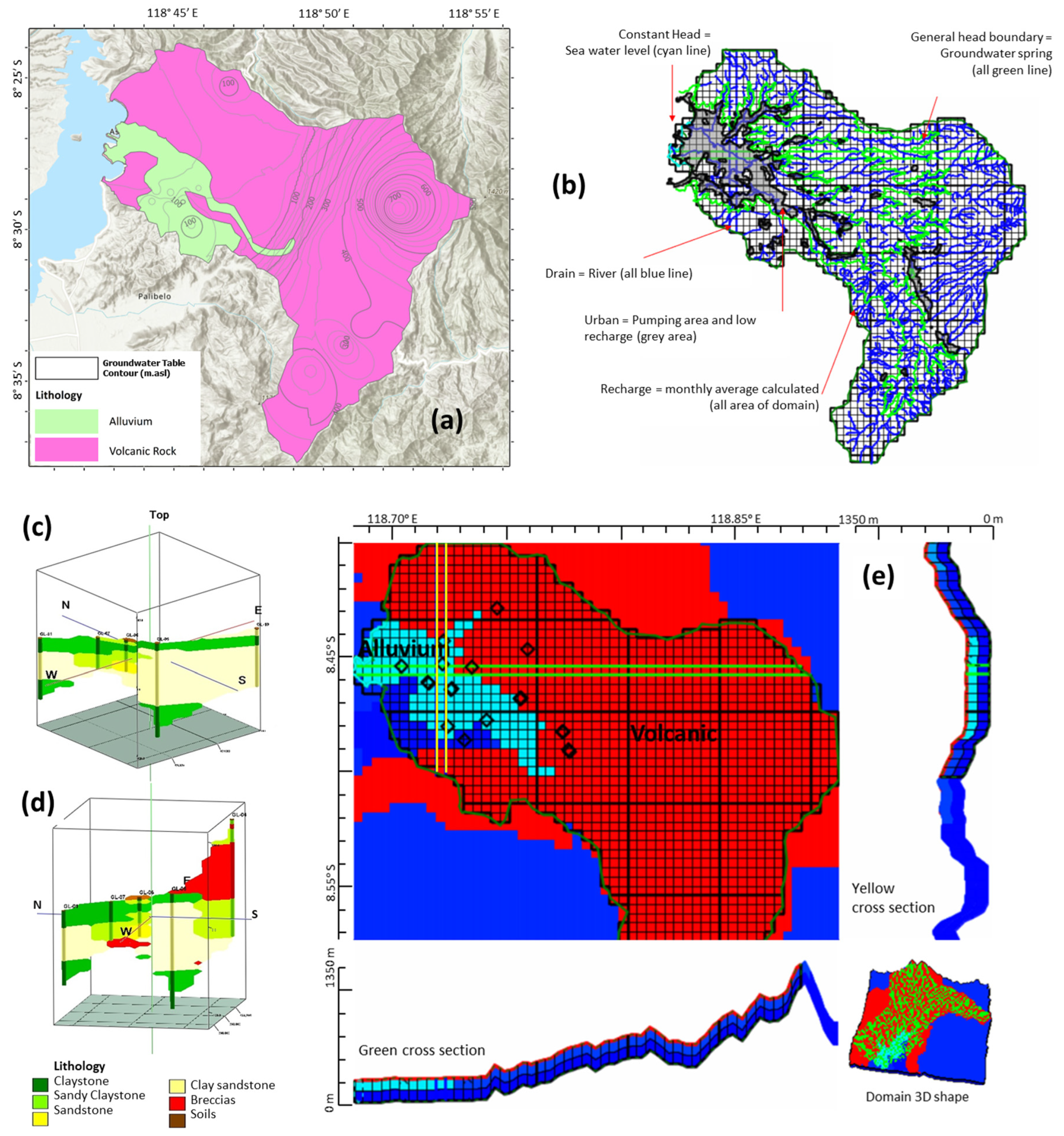
2.3. Groundwater Model

MODFLOW is one of the numerical modeling tools that is widely used for groundwater modeling. Modeling of groundwater sustainability has been conducted by many researchers using MODFLOW [19,20,21]. MODFLOW could provide spatiotemporal modeling to give a better understanding of groundwater systems. The conceptual model was constructed using MODFLOW-2005 and the Model Muse GUI [18]. Overall, groundwater modeling starts with hydrogeology data parameterization, data that has been collected and assigned as MODFLOW property using the GUI in the groundwater model. The groundwater model was calibrated using surveyed observation data, and then the calibrated model was used to predict groundwater scenarios (Figure 2).
The Rontu watershed area is 258.69 km2 with a steep slope averaging 15 degrees from the peak in the East to the sea in the West. Based on regional geological maps from the Indonesian Geological Agency [22], there are two lithologic zones in the Rontu watershed: the volcanic and the alluvium zones (Figure 3a). The hydrostratigraphy of the Rontu watershed was determined based on a resistivity method survey validated using regional geological maps from the Indonesian Geological Agency. Rocks with a higher resistivity tend to have larger grains, making the space between grains wider for groundwater flow. Conversely, lower resistivity means finer grains making the pores smaller for groundwater flow [23]. Based on resistivity values, the hydrostratigraphy of the alluvial zone consists mainly of sandy loam at depths of less than 10 m (0–10 Ωm), sandy loam at depths of 10–100 m (10–30 Ωm), and clay at depths below 100 m (0–10 Ωm) (Figure 3c). In the volcanic area, the aquifer consists mainly of volcanic breccia with sand to clay-sized grains (30–100 Ωm) overlying lava and breccia as bedrock (>100 Ωm) (Figure 3d).
The first step in building the model was to make a grid for numerical modeling boundaries by watershed area, with a total area of 258.69 km2. The discretization of the model in this study had a 400 × 400 m grid that was adequate for simulating flow and groundwater budget in the Rontu Watershed. After the horizontal grid had been built, the next step was to construct the vertical grid lithological layer based on the resistivity method, literature data, and the field geological survey. There were three layers of hydrostratigraphy in the study area: soil, aquifer, and bedrock. Each layer was projected to the Universal Transverse Mercator Coordinate and World Geodetic System (UTM WGS 84) projection system. The surface layer was assigned based on the 30 × 30 m Shuttle Radar Topography Mission (SRTM) digital elevation model (DEM). Each hydrostratigraphy layer’s top and bottom elevations were constructed using stratigraphic data from the primarily collected resistivities log. Aside from the field data, the aquifer properties were determined using the help of literature references. Due to the lack of detailed hydrogeological data for the region, uniform hydraulic conductivity values for each stratigraphic formation have been used, and a reasonable range was then manually selected, followed by manual calibration. The conductivity (K) values estimated and assigned for each layer were 2.0 × 10⁻⁵ m/s for the sandy volcanic aquifer, 2.0 × 10⁻⁴ m/s for the alluvium aquifer, and 1.0 × 10⁻⁹ m/s for the bedrock [24]. These results were validated using an infiltration test on the study area, which has a K value range from 2.0 × 10⁻⁵ up to 5.0 × 10⁻⁴ m/s. Since most of the lithology in the study area consisted of dense sandy aquifers, the storage coefficient was set to 5 × 10⁻⁵ m, and the specific yield was assigned to 20%. The effective porosity was assumed to be equal to the specific yield of the unconfined aquifer [25] (Figure 3e).
After hydro-stratigraphy had been built, boundary conditions were applied to reference groundwater flow, which can become a river, sea, lake, or other hydrological feature. These hydrologic features were obtained from satellite imagery and field surveys. Boundary conditions are parameters to determine the source or direction of groundwater flow. This study’s boundary conditions are sea, recharge from rainfall, stream, and water table observation on the field. However, the mountain peak around the area has no flow boundary. The eastern boundaries were assigned to a model that represents groundwater discharge due to springs; this boundary was assigned as the general head boundary. Monthly recharge to the upper layer was applied, and recharge was calculated using the water balance-based recharge estimation method [25,26] with the source of data from GSMaP [27,28,29,30]. On the west coast, a constant head boundary condition is assigned as a sea (Figure 3b).
After all the parameters are assigned, the groundwater model is run in MODFLOW and calibrated using field observation data. The model was calibrated by fitting observed groundwater to calculated heads in 23 observation wells. The calibration of hydraulic conductivity values (K values) is conducted by trial and error until good results are obtained. Based on the literature, this manual calibration method has been proven effective by many researchers [31]. After the model reached a good result in calibration, the groundwater model was used to simulate groundwater pumping based on the population spreading scenario. The recharge zone is at a higher elevation in the eastern volcanic area (Figure 3b), with a rough recharge estimate of 152 mm/year. Recharge occurs directly through outcrop deposition through cracks or upward and downward leakage via adjacent aquifers [32]. Based on infiltration tests in the study area, the soil in the study area consists of loamy sand with an average conductivity value of 2 × 10⁻⁴ m/s in alluvial soils and 5 × 10⁻⁴ m/s in unconsolidated volcanic soils.
The Rontu watershed has a volcanic plateau area directly adjacent to the coastal alluvial, making the Rontu watershed geologically representative of major cities in Indonesia. Regionally, the southeast islands of Indonesia have low rainfall, are dominated by dry conditions, and are related strongly to the ocean–atmospheric circulation, which is the El Nino Southern Oscillation and Indian Ocean Dipole, which modulate the anomalies of rainfall [33]. This condition is interesting to study since this location has good groundwater potential but with low rainfall as the source of groundwater.

2.4. Population Model

Population data in Bima were gathered from a raster database of the population generated by the Worldpop program. This database contains top-down constrained data that was produced using the random forest technique [34]. Population data for Indonesia were available in the grid with a resolution of 100 and have been adjusted to match United Nations national population estimates. Figure 4 shows the raster image of the gridded population count from Worldpop in 2010 and 2020 in the Rontu Watershed and Bima City area. The population number and the built-up area were then compared to judge population growth spreading following World Settlement Footprint (WSF) data. The WSF data were derived from Sentinel-1 and Landsat-8 images with an average accuracy of 86.37% [35]. From 2010 to 2020, the population grew relatively faster in the built-up area, as shown in (Figure 5A,B). The calculation of the historical, current, and projection of the population are made based on the grid cells, which have been reprojected from the 100 × 100 m grid to the 400 × 400 m grid using the zonal statistics method [36]. Afterward, the population numbers for built-up and non-built-up during the last ten years were plotted based on the number of populations per grid cell, which then projected up to 2045 using the linear least square method [37]. The population projection assumed that the population growth was constant.

3. Results

3.1. Population Density and Water Use Characteristics

Figure 4 shows the comparison of spatial population distribution for the years 2010 and 2020. A darker red area means a higher population density. In Figure 5A, the population distribution is also overlaid with settlement footprints (blue shade) to cross-check whether the location of the population is well-aligned. Then, temporal population data in Figure 5B prove that the population is steadily growing in the urban area. In contrast, the data show that the non-urban population is slightly declining every year. It is found that an increase in population occurred in areas with denser built-up areas. The 2045 urban population is projected to have grown by 21% from the population in 2020, with an average increase of 0.85% per year. In non-urban areas, the population from the last decade decreased by −0.78% from 2020 to 2045 (Figure 5B). Temporal image analysis supports the findings that the area with a higher built-up percentage also has a higher population growth. The highest built-up percentage is concentrated in the cities near the shore. In conjunction with decreasing populations in non-urban areas, we might assume that limited opportunities, such as economic development in the non-urban area, might cause the population growth to be concentrated in the cities. This growth characteristic means the urbanized areas continue to be denser with the human population, and water use increases yearly.
Based on the Ministry of Public Works and Housing of Indonesia (PUPR), the general domestic water need area is 144 L per day per person. Thus, from 2010 to 2020, the daily water needs increased from 14.45 million liters to 16.77 million liters for all areas. Another fact was found that only 40% of the water supply in Bima is directly covered by surface water. This means 60% of the remaining needs have been extracted from the groundwater for a prolonged time. In MODFLOW model implementation, the amount of pumping is determined by the standardized water demand per person per day (144 L/capita–day) multiplied by the total population in a 400 × 400 m MODFLOW grid multiplied by 60%. In addition, based on the local government’s medium-term development plans, it is planned that freshwater distribution from surface water will cover all water needs. Therefore, this research made a future scenario in which the percentage of groundwater use gradually decreases by the year due to increasing coverage of surface water distribution.

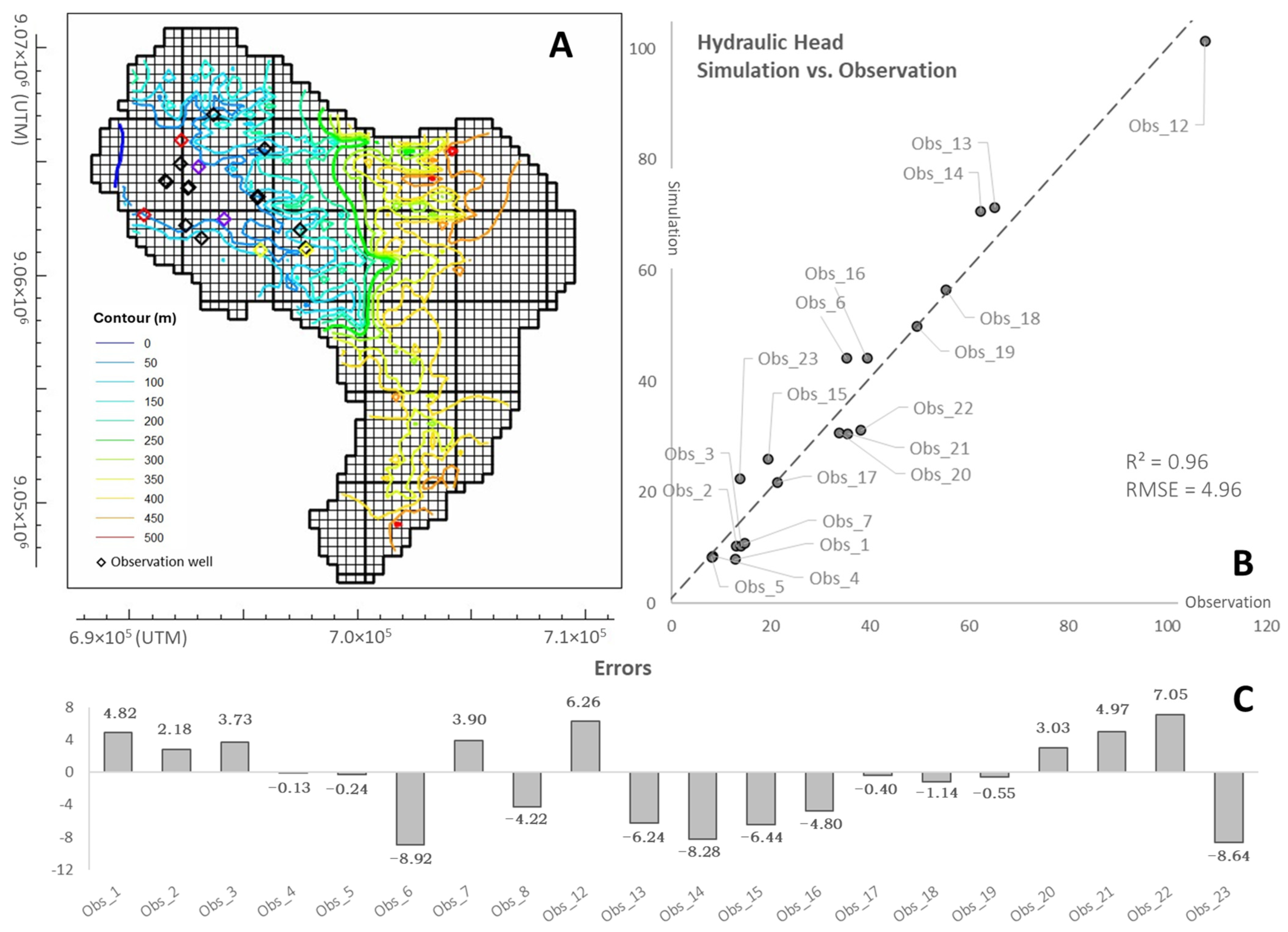
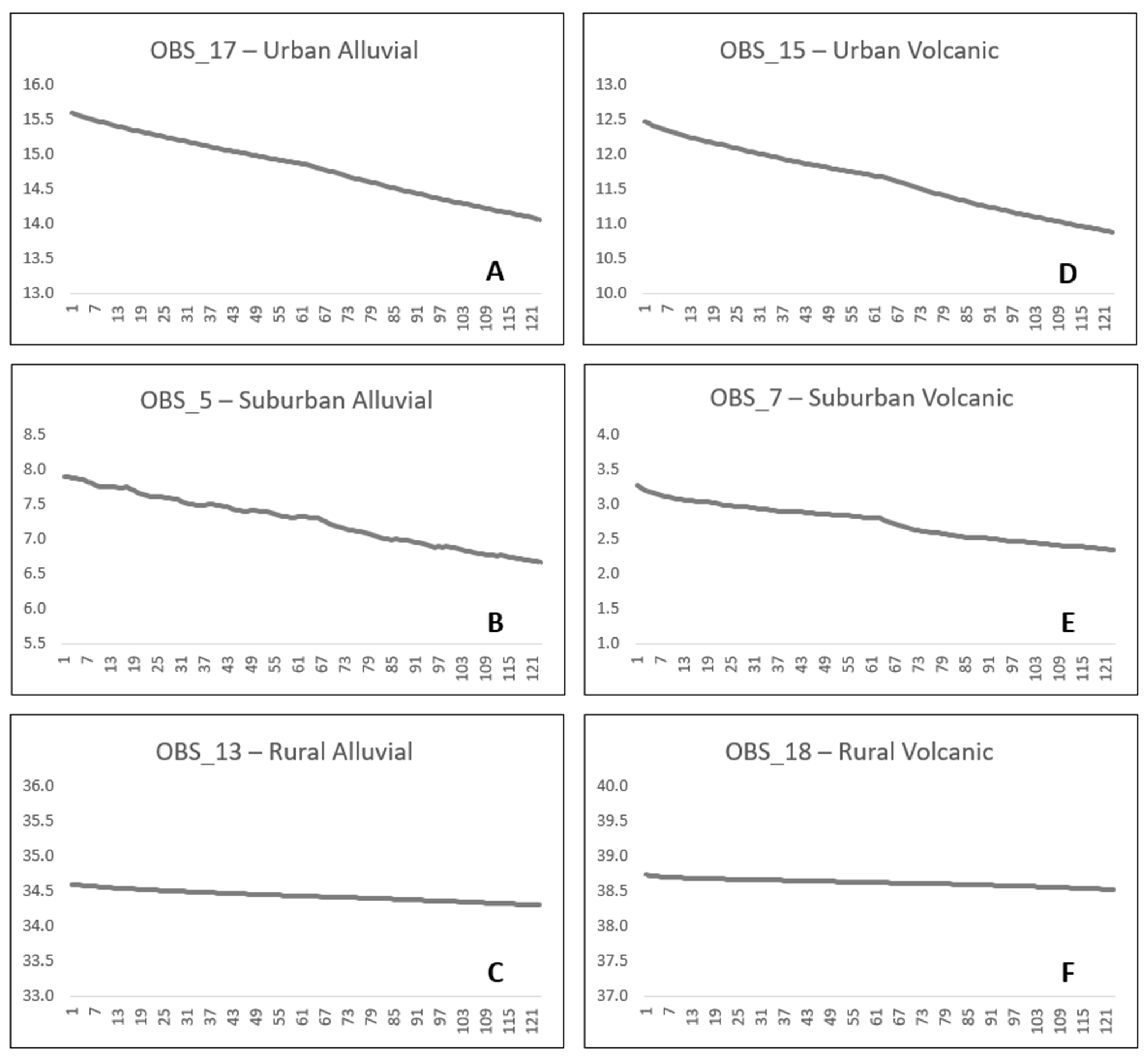
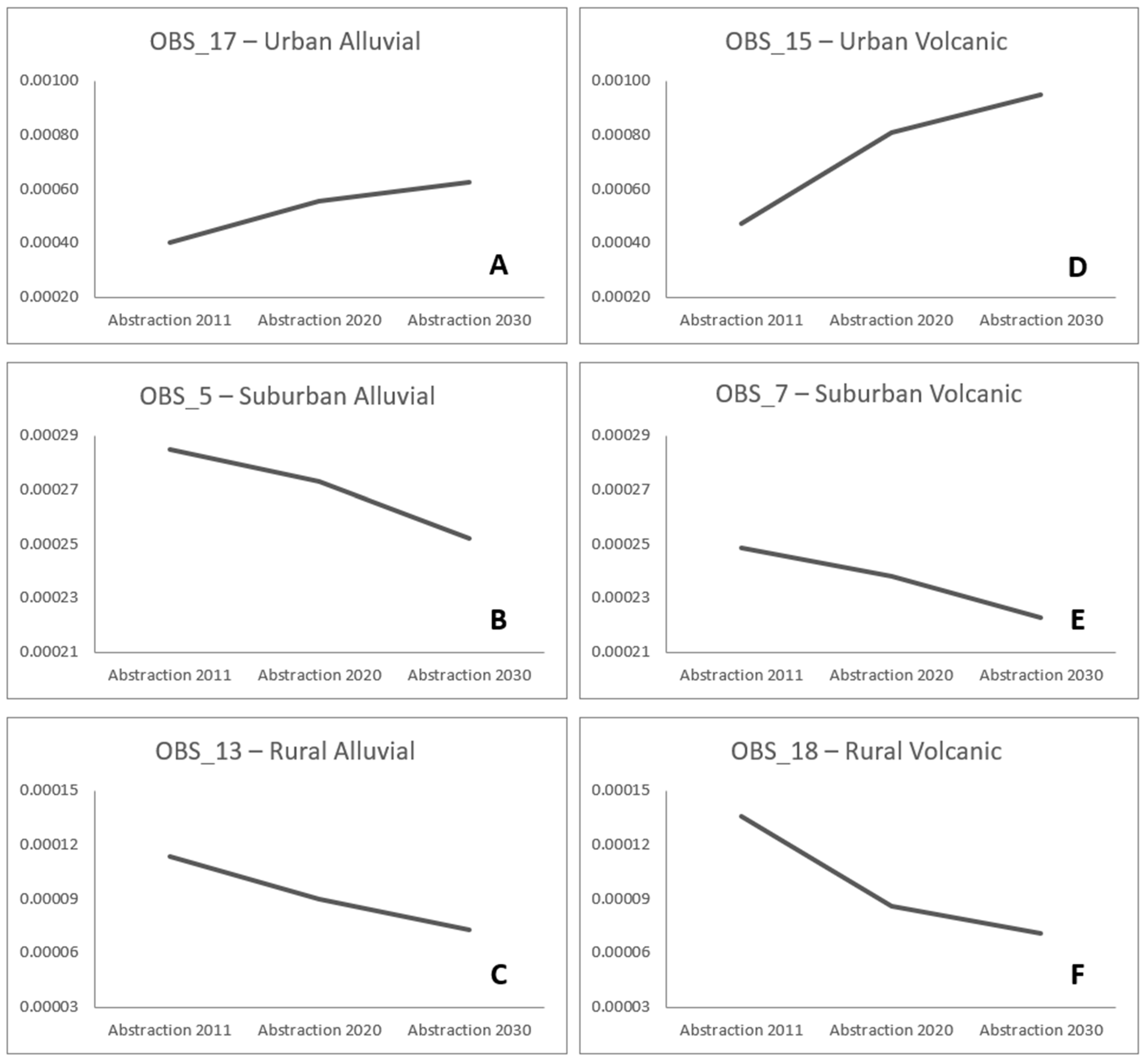
3.2. Groundwater Modeling Results

The groundwater contour map for the unconfined aquifer system shows that groundwater flow tends to follow slope direction with a maximum value of 476 m.asl (meters above average sea level) on the far east and a minimum of 0 m.asl on the west coast (Figure 6A). Groundwater flow in volcanic areas tends to be controlled by its aquifer geometry, which follows volcanic material deposition [32]. The groundwater flow is affected by constant head boundaries implemented at the western boundary as the sea and the general head boundary at the eastern boundaries. These are assigned based on actual groundwater conditions on the field observed on the surveyed groundwater well (Figure 5C).
The groundwater model was calibrated using observation data distributed at different population densities and lithologies to test the sensitivity of the parameters (Figure 5C). The calibration gave a result with an RMSE value of 4.9 m and a coefficient of determination of 0.96 (R2 = 0.96). The maximum residual difference was between 7.7 m and −7.9 m (Figure 6B), found in observation wells in volcanic areas. This finding may be caused by the complex condition of volcanic units by mixing lava and pyroclastic, as well as steep morphological conditions that may not be accommodated by the 400 × 400 m grid size. The calibration process gives K values ranging from 5 × 10⁻⁴ to 2 × 10⁻⁵ m/s for aquifers and from 1 × 10⁻⁷ to 1 × 10⁻⁹ m/s for bedrock. MODFLOW based on finite difference has limitations on conditions that vary in k (hydraulic conductivity) value and topography, but providing regional conditions is quite good [38].
From the groundwater simulation, it is found that groundwater drawdown from 2011 to 2020 is between 0.21 and 1.63 m. Urban areas have groundwater drawdowns up to 8 times higher than rural areas. Meanwhile, from 2020 up to 2030, if surface water covers up to 45% of water use, groundwater drawdown will reduce by up to 60%, and if surface water covers up to 65% of water use, in some areas, groundwater drawdown seems to stop in some areas (Table 1). From this condition, the notion is that the conjunctive use of surface water and groundwater effectively prevents rapid groundwater drawdown.
The zone budget of the groundwater model, which shows the water budget coming in and leaving out the groundwater model, is presented in Table 2. The general head boundary was the model’s most dominant water budget element. This boundary was defined as the groundwater springs. This indication is reasonable since the volcanic area had a large groundwater flux from the deeper aquifer in the higher slope area. On the other hand, the most dominant portion of the water budget leaving the model was the constant head at sea. This indication is also reasonable since all groundwater discharges to the sea. The constant head and general head boundary affected all observation wells equally. The influence of this boundary was relatively uniform in all observation wells. Therefore, these two factors can be neglected in their influence on the variation of groundwater level decline patterns of observation wells in various lithologies and population densities.

4. Discussion

Based on the simulated scenario, the groundwater drawdown in the study area for ten years only reached 1.63 m. This drawdown indicates that the Rontu watershed’s groundwater potential is good and capable of supporting domestic water needs, at least within the current modeled growth scenario. One supporting factor is that the Rontu watershed has good permeability to recharge rainfall into the groundwater since the lithology is volcanic and alluvium. This result is similar to that presented by Jasim et al. [39], where areas with volcanic hydrogeological soil conditions have good capability to support urban development.
Based on the characteristics of abstraction and groundwater level decline, there are three population density divisions: urban, suburban, and rural (Figure 7 and Figure 8). The urban area has a gradually increasing abstraction (Figure 8A,D) and experiences a linear pattern of groundwater level decline with a sharp gradient (Figure 7A,D). The pattern indicates the current condition, where the groundwater pumping is quite intense in urban areas. In the urban area, groundwater extraction or pumping exceeds its recharge capacity. The constant gradient in decreasing groundwater levels is usually found when the groundwater wells begin to stabilize, i.e., the groundwater pumping is balanced by the incoming groundwater flux. The fairly high groundwater potential in groundwater discharge areas and the high permeability of alluvium in urban areas contribute to preventing an exponential decrease in groundwater in urban areas despite an exponential increase in groundwater use.
In suburban locations, groundwater use is increasing but less than in urban areas (Figure 8B,E). The pattern of groundwater level decline is increasing but experiencing a gradual gradient in groundwater level decline over time (Figure 7B,E). This characteristic occurs when the decline in groundwater levels is yet to be steady until, at a certain time, it reaches a steady state and the decline occurs linearly. Meanwhile, groundwater extraction is decreasing in rural locations due to the population moving to cities (Figure 8C,F). However, the decline in groundwater levels continues to occur despite a sloping gradient of groundwater level decline. This indicates low groundwater potential in rural areas, where the decline continues to occur even though groundwater use is smaller. When viewed from the hydraulic properties of rocks, the low groundwater potential in rural areas indicates that volcanic rock types have relatively lower permeability than alluvial [40]. Besides that, rural areas are associated with groundwater recharge zones, in which groundwater flows regionally from this area to a lower area. Therefore, the groundwater potential in the rural area is lower.
Other research about dominant factors in the groundwater recharge process [41] found that hydraulic conductivity was the major factor affecting groundwater recharge. The volcanic rocks in this study area serve as groundwater zones with low potential, which justifies the rapid groundwater drawdown in the volcanic area. With many factors that affect groundwater drawdown, especially those highlighted in this research, such as groundwater pumping and permeability, it is found that the most sensitive factor that affects groundwater drawdown in the study area is groundwater pumping. This result is similar to the result conducted by another researcher [42]. Other findings in this research are that the Ob7 and Ob18 observation points have lower groundwater decline despite the lower permeability area. The location of the observation points near the river causes this. Since the river acts as the boundary condition to the groundwater system, the change in groundwater level was less pronounced than in other locations [43].
In this study, the reduction in groundwater use was carried out evenly throughout the region. This management scenario could be better considering the distribution of groundwater replacement. Surface water networks are not evenly distributed in all regions. However, this decrease in discharge can be used for local water management reference, where if a reduction in pumping is carried out in certain locations, the characteristics of the decline in groundwater levels can be seen locally at that location. Although groundwater modeling is carried out at the watershed scale, groundwater depletion can provide a local condition if supported by detailed resistivity data [44]. This is because groundwater is unlike surface water, which can move quickly; groundwater takes a long time to move to fill the decline. So, when a location experiences groundwater depletion, it takes work to return to the initial condition in a short time [45].
Considering the uneven characteristics of groundwater level decline in different population densities and hydrogeological characteristics, constructing surface water support facilities can be prioritized in dense areas with low permeability lithological conditions. With such a prioritization, groundwater can be better maintained and infrastructure development can benefit the community that needs it the most. Monitoring well facilities in each lithologic variation and population density is recommended because of the varying subsurface hydrogeologic conditions. With high permeability characteristics, this watershed has a high potential for groundwater recharge in the upper volcanic zone. To support the growing urban population in a sustainable fashion, a resilient groundwater recharge infrastructure system [46] is suggested to be built. This infrastructure not only consists of physical facilities, e.g., monitoring well networks and well-designed recharge wells, but also strict zoning regulations and land-use planning. Other research [21] suggested that the implementation of proper groundwater abstraction control policy and measure is able to restore the groundwater level to rise back. Indonesia already has a strict groundwater regulation legally managed by the Geological Agency of Indonesia. However, the details of such a rule, the actual on-field enforcement, and the contextual applicability are subject to follow-up studies.

5. Conclusions

The groundwater model can provide an overview of the decline in groundwater levels due to variations in population density, aquifer property, and boundary conditions. Based on the analysis of resistivity logs, regional geological maps, and field mapping, the groundwater model of Rontu Watershed, Bima comprises three main layers: the soil layer, aquifer, and bedrock. In general, two lithological groups are used to determine the aquifer property at the research site, namely alluvium and volcanic. Groundwater boundary conditions in the study area are based on surface water features of the ocean, rivers, and infiltration. Projections of population increase were made using the linear least square method so that the groundwater model could provide an overview of groundwater conditions in the next few years.
Three characteristics of groundwater drawdown were found: (1) In urban areas, the pattern of groundwater drawdown increased linearly with a relatively sharper gradient than other groups of areas; (2) In suburban areas, the groundwater drawdown increased exponentially in the first year but changed to linear with a low gradient in the last years; (3) In rural areas, the groundwater drawdown increased exponentially from year to year, although with a small gradient. It was also found that the decline in groundwater level in the alluvium plain area tends to be smaller than in the volcanic upland area with the same population density conditions. This follows the groundwater potential map published by the national government, which states that the groundwater potential in the alluvium plain area is higher than in the volcanic upland area. Besides the previous major factor, rivers as a boundary condition also give contribution to groundwater in shallow aquifers. Groundwater conservation efforts are carried out through simulations of groundwater use reduction so that the groundwater level does not continue to fall. The simulations of the groundwater model show that it is necessary to reduce groundwater use by 65% of the total water needs of the population in Bima City and replace it by optimizing the supply and use of surface water, artificial recharge, and groundwater abstraction control policy to stop groundwater levels from declining continuously. Based on the results of this research, water resource management needs to consider hydrogeological and socio-economic aspects to determine an effective and efficient management strategy.

Author Contributions

Conceptualization, F.I.W.R. (Faizal Immaddudin Wira Rohmat) and D.R.; methodology, A.H. and R.A.; software, A.H. and R.A.; validation, F.I.W.R. (Fauzan Ikhlas Wira Rohmat); formal analysis, A.H. and F.I.W.R. (Fauzan Ikhlas Wira Rohmat); investigation, A.H. and R.A.; resources, D.R.; data curation, A.H., P.V.A. and A.W.; writing—original draft preparation, A.H., R.A. and F.I.W.R. (Fauzan Ikhlas Wira Rohmat); writing—review and editing, F.I.W.R. (Faizal Immaddudin Wira Rohmat) and W.W.; visualization, A.H., R.A. and F.I.W.R. (Fauzan Ikhlas Wira Rohmat); supervision, D.R.; project administration, D.R.; funding acquisition, D.R. All authors have read and agreed to the published version of the manuscript.

Funding

The work reported was funded by a grant from the KEMDIKBUD/the Ministry of Education and Culture of the Republic of Indonesia for the project entitled “Resilient Indonesian Slums Envisioned (RISE)—Building an inclusive governance with people and water to make social-ecological interactions more resilient to water-related disasters” under the RISTEKBRIN-NWO Merian Fund call for collaboration between Indonesia and the Netherlands. The authors would also express their acknowledgment of the support provided by the ITB International Research Grant with grant number LPPM.PN-10-56-2022 and the FTSL PPMI 2022/2023 program.

Data Availability Statement

Data will be made available upon request.

Conflicts of Interest

Author R.A. was employed by the company Deltares Indonesia. The remaining authors declare that the research was conducted in the absence of any commercial or financial relationships that could be construed as a potential conflict of interest.

References

  1. Condon, L.E.; Kollet, S.; Bierkens, M.F.P.; Fogg, G.E.; Maxwell, R.M.; Hill, M.C.; Fransen, H.J.H.; Verhoef, A.; Van Loon, A.F.; Sulis, M.; et al. Global Groundwater Modeling and Monitoring: Opportunities and Challenges. Water Resour. Res. 2021, 57, e2020WR029500. [Google Scholar] [CrossRef]
  2. Li, P.; Karunanidhi, D.; Subramani, T.; Srinivasamoorthy, K. Sources and Consequences of Groundwater Contamination. Arch. Environ. Contam. Toxicol. 2021, 80, 1–10. [Google Scholar] [CrossRef] [PubMed]
  3. Ntona, M.M.; Busico, G.; Mastrocicco, M.; Kazakis, N. Modeling Groundwater and Surface Water Interaction: An Overview of Current Status and Future Challenges. Sci. Total Environ. 2022, 846, 157355. [Google Scholar] [CrossRef] [PubMed]
  4. Podgorski, J.; Berg, M. Global Threat of Arsenic in Groundwater. Science 2020, 368, 845–850. [Google Scholar] [CrossRef] [PubMed]
  5. Barbieri, M.; Barberio, M.D.; Banzato, F.; Billi, A.; Boschetti, T.; Franchini, S.; Gori, F.; Petitta, M. Climate Change and Its Effect on Groundwater Quality. Environ. Geochem. Health 2023, 45, 1133–1144. [Google Scholar] [CrossRef] [PubMed]
  6. Rohmat, F.I.W.; Labadie, J.W.; Gates, T.K. Deep Learning for Compute-Efficient Modeling of BMP Impacts on Stream- Aquifer Exchange and Water Law Compliance in an Irrigated River Basin. Environ. Model. Softw. 2019, 122, 104529. [Google Scholar] [CrossRef]
  7. Morway, E.D.; Niswonger, R.G.; Triana, E. Toward Improved Simulation of River Operations through Integration with a Hydrologic Model. Environ. Model. Softw. 2016, 82, 255–274. [Google Scholar] [CrossRef]
  8. Shultz, C.D.; Gates, T.K.; Bailey, R.T. Evaluating Best Management Practices to Lower Selenium and Nitrate in Groundwater and Streams in an Irrigated River Valley Using a Calibrated Fate and Reactive Transport Model. J. Hydrol. 2018, 566, 299–312. [Google Scholar] [CrossRef]
  9. Fields, C.M.; Labadie, J.W.; Rohmat, F.I.W.; Johnson, L.E. Geospatial Decision Support System for Ameliorating Adverse Impacts of Irrigated Agriculture on Aquatic Ecosystems. Agric. Water Manag. 2021, 252, 106877. [Google Scholar] [CrossRef]
  10. La Vigna, F. Review: Urban Groundwater Issues and Resource Management, and Their Roles in the Resilience of Cities. Hydrogeol. J. 2022, 30, 1657–1683. [Google Scholar] [CrossRef]
  11. Chaminé, I.; Afonso, M.J.; Barbieri, M.; De Paola, F.; Foster, S.; Hirata, R.; Eichholz, M.; Alam, M.-F. Urban Self-Supply from Groundwater—An Analysis of Management Aspects and Policy Needs. Water 2022, 14, 575. [Google Scholar] [CrossRef]
  12. Foster, S. The Key Role for Groundwater in Urban Water-Supply Security. J. Water Clim. Chang. 2022, 13, 3566–3577. [Google Scholar] [CrossRef]
  13. Hamilton, W.B.; Lujan, M.; Peck, D.L. Tectonics of the Indonesian Region. In Professional Paper; United States Geological Survey: Sunrise Valley Drive Reston, VA, USA, 1979. [Google Scholar] [CrossRef]
  14. As-syakur, A.R.; Tanaka, T.; Osawa, T.; Mahendra, M.S. Indonesian Rainfall Variability Observation Using TRMM Multi-Satellite Data. Int. J. Remote. Sens. 2013, 34, 7723–7738. [Google Scholar] [CrossRef]
  15. Carrard, N.; Foster, T.; Willetts, J. Groundwater as a Source of Drinking Water in Southeast Asia and the Pacific: A Multi-Country Review of Current Reliance and Resource Concerns. Water 2019, 11, 1605. [Google Scholar] [CrossRef]
  16. Geyh, M.A.; Soefner, B. Groundwater Mining Study by SImplified Sample Collection in the Jakarta Basin Aquifer, Indonesia. In Isotopes in Water Resources Management. V. 2. PROCEEDINGS of a Symposium; Proceedings Series; International Atomic Energy Agency: Vienna, Austria, 1996; pp. 174–176. [Google Scholar]
  17. Abidin, H.Z.; Andreas, H.; Gumilar, I.; Sidiq, T.P.; Fukuda, Y. Land Subsidence in Coastal City of Semarang (Indonesia): Characteristics, Impacts and Causes. Geomat. Nat. Hazards Risk 2013, 4, 226–240. [Google Scholar] [CrossRef]
  18. Winston, R.B. Winston ModelMuse Version 4: A Graphical User Interface for MODFLOW 6. In Scientific Investigations Report—US Geological Survey; United States Geological Survey: Baltimore, MD, USA, 2019. [Google Scholar]
  19. Massuel, S.; George, B.; Gaur, A.; Nune, R. Groundwater Modeling for Sustainable Resource Management in the Musi Catchment, India. Proc. Int. Congr. Model. Simul. 2007, 10, 1429–1435. [Google Scholar]
  20. Singh, A. Groundwater Modelling for the Assessment of Water Management Alternatives. J. Hydrol. 2013, 481, 220–229. [Google Scholar] [CrossRef]
  21. Lo, W.; Purnomo, S.N.; Sarah, D.; Aghnia, S.; Hardini, P. Groundwater Modelling in Urban Development to Achieve Sustainability of Groundwater Resources: A Case Study of Semarang City, Indonesia. Water 2021, 13, 1395. [Google Scholar] [CrossRef]
  22. Ratman, N.; Yasin, A. Peta Geologi Lembar Komodo, Nusatenggara. Badan Geologi Indonesia; The University of Chicago: Chicago, IL, USA, 1978. [Google Scholar]
  23. Parsekian, A.D.; Singha, K.; Minsley, B.J.; Holbrook, W.S.; Slater, L. Multiscale Geophysical Imaging of the Critical Zone. Rev. Geophys. 2015, 53, 1–26. [Google Scholar] [CrossRef]
  24. Domenico, P.A.; Schwartz, F.W. Physical and Chemical Hydrogeology, 2nd ed.; John Wiley & Sons: New York, NY, USA, 1998; p. 528. [Google Scholar]
  25. Heath, R.C. Basic Ground-Water Hydrology. In Water Supply Paper; United States Geological Survey: Baltimore, MD, USA, 1983. [Google Scholar] [CrossRef]
  26. Wardhana, Y.A.W.; Fauzan, I.; Rengganis, H. Potensi Air Tanah Di Wilayah Pengungsian Erupsi Gunung Agung Bali. J. Tek. Hidraul. 2019, 10, 74–89. [Google Scholar] [CrossRef]
  27. Tian, Y.; Peters-Lidard, C.D.; Adler, R.F.; Kubota, T.; Ushio, T. Evaluation of GSMaP Precipitation Estimates over the Contiguous United States. J. Hydrometeorol. 2010, 11, 566–574. [Google Scholar] [CrossRef]
  28. Aonashi, K.; Awaka, J.; Hirose, M.; Kozu, T.; Kubota, T.; Liu, G.; Shige, S.; Kida, S.; Seto, S.; Takahashi, N.; et al. Gsmap Passive Microwave Precipitation Retrieval Algorithm: Algorithm Description and Validation. J. Meteorol. Soc. Jpn. 2009, 87A, 119–136. [Google Scholar] [CrossRef]
  29. Kubota, T.; Shige, S.; Hashizume, H.; Aonashi, K.; Takahashi, N.; Seto, S.; Hirose, M.; Takayabu, Y.N.; Ushio, T.; Nakagawa, K.; et al. Global Precipitation Map Using Satellite-Borne Microwave Radiometers by the GSMaP Project: Production and Validation. Proc. IEEE Trans. Geosci. Remote Sens. 2007, 45, 2259–2275. [Google Scholar] [CrossRef]
  30. Kubota, T.; Aonashi, K.; Ushio, T.; Shige, S.; Takayabu, Y.N.; Kachi, M.; Arai, Y.; Tashima, T.; Masaki, T.; Kawamoto, N.; et al. Global Satellite Mapping of Precipitation (GSMaP) Products in the GPM Era. In Advances in Global Change Research; Springer: Cham, Switzerland, 2020; Volume 67. [Google Scholar]
  31. Hunt, R.J.; Fienen, M.N.; White, J.T. Revisiting “An Exercise in Groundwater Model Calibration and Prediction” after 30 Years: Insights and New Directions. Groundwater 2020, 58, 168–182. [Google Scholar] [CrossRef] [PubMed]
  32. de Vries, J.J.; Simmers, I. Groundwater Recharge: An Overview of Process and Challenges. Hydrogeol. J. 2002, 10, 5–17. [Google Scholar] [CrossRef]
  33. Rohmat, F.I.W.; Harjupa, W.; Rohmat, D.; Rohmat, F.I.W. The Impacts of Global Atmospheric Circulations on the Water Supply in Select Watersheds in the Indonesian Maritime Continent Using SPI. Heliyon 2023, 9, e15604. [Google Scholar] [CrossRef]
  34. Stevens, F.R.; Gaughan, A.E.; Linard, C.; Tatem, A.J. Disaggregating Census Data for Population Mapping Using Random Forests with Remotely-Sensed and Ancillary Data. PLoS ONE 2015, 10, e0107042. [Google Scholar] [CrossRef]
  35. Marconcini, M.; Metz-Marconcini, A.; Üreyen, S.; Palacios-Lopez, D.; Hanke, W.; Bachofer, F.; Zeidler, J.; Esch, T.; Gorelick, N.; Kakarla, A.; et al. Outlining Where Humans Live, the World Settlement Footprint 2015. Sci. Data 2020, 7, 242. [Google Scholar] [CrossRef]
  36. Hyndman, R.J.; Fan, Y. Sample Quantiles in Statistical Packages. Am. Stat. 1996, 50, 361–365. [Google Scholar] [CrossRef]
  37. Ihsan, K.T.N.; Anantri, N.M.K.; Syamsu, A.A.; Mustika, F.C. Prediction of Population Distribution in 2030 Using the Integration of the CA-ANN Land Cover Change Method with Numeric Extrapolation in Karawang-Bekasi, Indonesia. Int. Arch. Photogramm. Remote Sens. Spat. Inf. Sci. 2022, XLVI-M-2–2022, 111–118. [Google Scholar] [CrossRef]
  38. Simpson, M.J.; Clement, T.P. Comparison of Finite Difference and Finite Element Solutions to the Variably Saturated Flow Equation. J. Hydrol. 2003, 270, 49–64. [Google Scholar] [CrossRef]
  39. Jasim, A.; Hemmings, B.; Mayer, K.; Scheu, B. Groundwater Flow and Volcanic Unrest. In Advances in Volcanology; Springer: Cham, Switzerland, 2019; pp. 83–99. [Google Scholar] [CrossRef]
  40. Käser, D.; Hunkeler, D. Contribution of Alluvial Groundwater to the Outflow of Mountainous Catchments. Water Resour. Res. 2016, 52, 680–697. [Google Scholar] [CrossRef]
  41. Castillo, J.L.U.; Ramos Leal, J.A.; Martínez Cruz, D.A.; Cervantes Martínez, A.; Marín Celestino, A.E. Identification of the Dominant Factors in Groundwater Recharge Process, Using Multivariate Statistical Approaches in a Semi-Arid Region. Sustainability 2021, 13, 11543. [Google Scholar] [CrossRef]
  42. Islam, M.; Van Camp, M.; Hossain, D.; Sarker, M.M.R.; Khatun, S.; Walraevens, K. Impacts of Large-Scale Groundwater Exploitation Based on Long-Term Evolution of Hydraulic Heads in Dhaka City, Bangladesh. Water 2021, 13, 1357. [Google Scholar] [CrossRef]
  43. Chang, S.W.; Chung, I.M. Water Budget Analysis Considering Surface Water–Groundwater Interactions in the Exploitation of Seasonally Varying Agricultural Groundwater. Hydrology 2021, 8, 60. [Google Scholar] [CrossRef]
  44. Lévesque, Y.; Chesnaux, R.; Walter, J. Using Geophysical Data to Assess Groundwater Levels and the Accuracy of a Regional Numerical Flow Model. Hydrogeol. J. 2023, 31, 351–370. [Google Scholar] [CrossRef]
  45. Schreiner-McGraw, A.P.; Ajami, H. Delayed Response of Groundwater to Multi-Year Meteorological Droughts in the Absence of Anthropogenic Management. J. Hydrol. 2021, 603, 126917. [Google Scholar] [CrossRef]
  46. Mohammad-Hosseinpour, A.; Molina, J.L. Improving the Sustainability of Urban Water Management through Innovative Groundwater Recharge System (GRS). Sustainability 2022, 14, 5990. [Google Scholar] [CrossRef]
Figure 1. Study area of the research: (A) Indonesia; (B) West Nusa Tenggara Province; (C) Location of Bima City and Rontu Watershed.
Water 15 04262 g001
Figure 2. General modeling flowchart.
Water 15 04262 g002
Figure 3. (a) The study area mainly consisted of two lithology types: alluvium on the western lowland and volcanic on the eastern highland. The contours present observed groundwater table elevation in meters above sea level (m.asl). (b) Model boundary conditions, including the treatment of streams and rivers, assumed as drains or gaining streams, constant head at sea boundary, general head boundaries, urban pumping, and recharge areas. (c) Hydrostratigraphy of the alluvium study area consists of soil clay and sandy aquifer. (d) Hydrostratigraphy of the volcanic area comprises volcanic soil and underlying volcanic rocks. (e) ModelMuse interface showing plan, section, and domain views of the aquifer properties assigned to the conceptual model based on volcanic and alluvium lithology properties. The black diamond blocks are the locations of calibration points used in the model calibration.
Water 15 04262 g003
Figure 4. Population counts in 100 m grid cell for 2010 (a) and 2020 (b) based on the Worldpop data.
Water 15 04262 g004
Figure 5. (A) Population growth spread from 2010 to 2020. The red box represents areas with high population density, where the observation locations are mainly spread. The blue-shaded areas are the footprint of the settlement. (B) Population growth in Bima City for 2010–2020. The least-square linear trendline shows growth in urban areas while the non-urban area population is declining. In net, the total population growth is positive. (C) Observation well location overlaid with population dynamic, the zoom view of the red box in (A).
Water 15 04262 g005
Figure 6. (A) Regional groundwater flow of study area in MODFLOW with rural area as yellow diamonds, sub-urban as purple, and urban area as red diamonds. The black diamonds are observed points excluded from Table 1; (B) Calibration result of the study area shows RMSE of 4.96 and R2 of 0.96 with the 1:1 guideline provide visual guide of the calibration performance; (C) Error bars of every simulation point.
Water 15 04262 g006
Figure 7. Groundwater drawdown characteristics based on population density and geology type: (A) urban alluvial, (B) sub-urban alluvial, (C) rural alluvial, (D) urban volcanic, (E) sub-urban volcanic, and (F) rural volcanic. The x-axes are timesteps in month and the y-axes are groundwater elevation in meter.
Water 15 04262 g007
Figure 8. Groundwater abstraction growth characteristics based on population density and geology types: (A) urban Alluvial, (B) sub-urban alluvial, (C) rural alluvial, (D) urban volcanic, (E) sub-urban volcanic, and (F) rural volcanic. The y-axes are groundwater abstractions in m3/s.
Water 15 04262 g008
Table 1. Groundwater drawdown from 2021 to 2030 for various scenarios.
Observation WellLithologyPopulation Density Type2011–2020 Drawdown (m)2030 Drawdown with 45% Pipeline
Coverage
(m)
2030 Drawdown with 55% Pipeline
Coverage
(m)
Ob7VolcanicSuburban0.920.250.10
Ob5AlluvialSuburban1.220.420.22
Ob15VolcanicUrban1.590.670.42
Ob17AlluvialUrban1.530.770.52
Ob13AlluvialRural0.300.200.17
Ob18VolcanicRural0.210.260.22
Table 2. Zone budget of groundwater model.
Zone Budget (m3/s)
In:Out:
Storage = 1.2405 × 10⁻²Storage = 1.150 × 10⁻³
Constant Head = 7.9965 × 10⁻²Constant Head = 0.1772
Wells = 0.0000Wells = 6.6081 × 10⁻²
Drains = 0.0000Drains = 2.9308 × 10⁻²
Head Dep Bounds = 0.1628Head Dep Bounds = 2.0613 × 10⁻²
Recharge = 1.2810 × 10⁻²Recharge = 0.0000
Total In = 0.2680Total Out = 0.2680
Disclaimer/Publisher’s Note: The statements, opinions and data contained in all publications are solely those of the individual author(s) and contributor(s) and not of MDPI and/or the editor(s). MDPI and/or the editor(s) disclaim responsibility for any injury to people or property resulting from any ideas, methods, instructions or products referred to in the content.

