A Combined Model for Water Quality Prediction Based on VMD-TCN-ARIMA Optimized by WSWOA

Abstract

With environmental degradation and water scarcity becoming increasingly serious, it is urgent to carry out effective management of water resources. The key task of water environment monitoring is to conduct statistics and analysis of changes in water quality characteristics. Aiming to address the problem of the strong fluctuation and strong temporal correlation of water quality characteristics prediction, a new framework for water quality prediction based on variational mode decomposition–temporal convolutional networks–autoregressive integrated moving average (VMD-TCN-ARIMA) optimized by weighted swarm the whale search algorithm (WSWOA) algorithm is proposed. First, the WSWOA was proposed by introducing the two-weighted-factor perturbation strategy and the particle swarm search method based on the whale optimization algorithm (WOA), which effectively improves the convergence speed and global search capabilities. Second, to adaptively decompose the original water quality sequences, the VMD algorithm optimized by WSWOA was utilized, which can extract features and reduce noise in the original sequence. Furthermore, the TCN-ARIMA combined model is proposed for time series analysis. The combined model is introduced to assign different algorithms to the decomposed components to reduce prediction error and modeling effort. In comparison to VMD-TCN model, the experimental results have shown that on the data of water quality characteristic dissolved oxygen (DO), the proposed model’s root mean square error (RMSE) and computational time is reduced by 41.05% and 26.06%, further improving the accuracy and efficiency of prediction.

1. Introduction

Water is fundamental to life, essential for providing pure drinking water, sustaining agricultural production, and preserving ecological balance [1]. However, with the rapid development of the social economy, technology, and industry, global water quality issues are becoming increasingly severe [2]. The efficient implementation of testing and management strategies for water resources has emerged as a significant area of interest in recent years [3]. Water quality prediction, as the foundation for environmental monitoring and management of water quality, has become an important research theme in the fields of environmental science and water resources management [4]. Water quality characteristics include parameters such as dissolved oxygen concentration, pH, turbidity, nitrogen, phosphorus, and organic matter content, which are critical for assessing the health of water bodies, ensuring the quality of water supplies, and maintaining ecosystem stability [5].

The data used to characterize water quality are nonlinear and influenced by a variety of external factors, such as temperature, weather, and location [6]. To accurately predict the trend of changes in water quality, it is vital to extract effective details from the raw data and select the most suitable prediction model. Currently, the methods for predicting water quality characteristics can be categorized into three groups. The first type includes traditional statistical methods of prediction, such as the common gray system theory model [7] and the Markov model [8]. Ghaemi et al. [9] developed an autoregressive integrated moving average model (ARIMA) for predicting water quality characteristics in the distribution network using static and dynamic samples to improve the performance of the water distribution network and warn of contamination within the network. The experimental results show that the model can learn the changing characteristics of time series data and is applicable for predicting the characterization of water quality. However, the learning capability of these traditional time series analysis models is too shallow to fit highly complex nonlinear time series.

To solve this problem, we have the second type of water quality prediction algorithms, represented by back propagation neural networks (BP), convolutional neural network (CNN), long- and short-term memory networks (LSTM), and temporal convolutional networks (TCN), which, based on machine learning, have been gradually applied to the field to overcome nonlinear difficulties [10,11]. Cheng et al. [12] proposed a BP neural network based on the Levenberg–Marquant algorithm to simulate the dissolved oxygen concentration in the Yellow River in China. The prediction effect was superior to using a BP network directly. AlDahoul et al. [13] utilized LSTM model to simulate and forecast the suspended sediment concentration of the Johor River in Malaysia. The experimental results show that its performance is better than the traditional regression model and BP neural network in daily, weekly, and monthly prediction scenarios. Fu et al. [14] proposed a prediction method with TCN as the core based on the key characteristics of marine aquaculture, with an accuracy of 91.91%. Research demonstrates that this model has higher prediction accuracy and lower time complexity than recurrent neural network (RNN), simple recurrent units (SRU), bi-directional simple recurrent units (BISRU), LSTM, and gate recurrent unit (GRU) similar prediction networks. However, the prediction effect produced by a single neural network algorithm will have shortcomings such as poor generalization ability and easy overfitting, and will not be able to handle the variability and complexity of water quality characteristics data effectively [15].

Consequently, a third type model emerged: the combination prediction model. Current combined models can be classified broadly into two categories. A model combining multiple prediction algorithms is one, which amalgamates the strengths of multiple algorithms to overcome the limitations associated with the use of a single algorithm [16]. Nevertheless, the performance of such a model exhibits large fluctuations and poor generalization to different water quality characteristics. For example, the LSTM-BP [17] and LSTM-CNN [18] combined prediction model can effectively extract changes in specific water quality characteristics, but it has poor generalization and cannot obtain the same effect for other water quality characteristics. The other category is a model based on signal decomposition and feature extraction. The effective features of the water quality data are extracted via signal decomposition then fitted by the predictor; ultimately, the signal is reconstructed to obtain the prediction result. Common time series decomposition methods mainly include empirical mode decomposition (EMD), complete ensemble empirical mode decomposition with adaptive noise (CEEMDAN), and VMD, and such methods have been widely used in forecasting studies of various types of time series data [19]. Zhang et al. [20] proposed an integrated EMD-LSTM combined prediction model and used it to simulate and predict five water quality characteristics, including chemical oxygen demand (COD), total phosphorus (TP), and other water quality characteristics in the Tahe oil field in China. Wang et al. [21] proposed a combined VMD-GRU prediction model, using integrated variational modal decomposition VMD and gated recurrent unit GRU to simulate and predict seven water quality characteristics, such as pH and TP, in the drainage network gathered from a wastewater treatment plant in Shenzhen, China. However, due to the addition of data decomposition modules on the original basis, the requirements for the hyperparameter settings have increased, making the selection of the appropriate hyperparameter settings for each model a key factor in determining the efficacy of the models. Geng et al. [22] optimized the model by using a particle swarm algorithm (PSO), and a combined VMD-TCN model was used to predict time series. The results indicate that modifying the model’s parameters using optimization algorithms can improve the model’s prediction accuracy and efficiency. Liu et al. [23] utilized the improved whale optimization algorithm (IWOA) to similarly optimize the parameters of BP neural network prediction model, thereby establishing the combined prediction model CEEMDAN-IWOA-BP. Experimental results indicate that the IWOA is preferable to the WOA, the genetic algorithm (GA), and the PSO when optimizing the parameters of BP neural network for predicting water quality characteristics. Moreover, the combined model’s predictive accuracy has been enhanced when compared to the individual models.

The models developed in the above discussions and studies have been able to accurately predict water quality characteristics. However, these models can only be applied to water quality data in a fixed area, and different parameters must be manually selected based on various water quality characteristics for the model to function optimally [24]. Therefore, it is necessary to enhance the prediction model’s generalization. Secondly, the best-performing models at present are all founded on the learning capabilities of deep neural networks. However, deep network training and fitting require a significant amount of time, whereas traditional statistical models do not. To reduce model time and increase prediction efficiency, it is crucial to combine the benefits of both approaches [25]. Finally, compared to other optimization algorithms, the WOA has a straightforward structure, fewer parameters, and a quicker iteration speed. However, the original WOA algorithm is prone to local optima, necessitating improvements to the algorithm’s structure to enhance its global search capability [26].

This study proposes a combined prediction model of VMD-TCN-ARIMA based on the WSWOA optimization algorithm in response to the mentioned issues. First, to address the fundamental issues in the original WOA, the WSWOA algorithm is suggested. This method integrates the position updating technique from particle swarm optimization, which enhances the search space and accelerates the convergence rate, as well as a stochastic perturbation strategy with coupled dual weights to eliminate the local optimum defect. Second, the water quality characteristics are separated into two sections, complex and simple, based on the standardized discrete coefficients of each modal component after the decomposition of the water quality sequence with the VMD optimized by WSWOA. The former is fed into the WSWOA-optimized TCN neural network, whereas the latter is fed into the ARIMA. Finally, the result of the prediction is obtained by superimposing all output-fitting components. The proposed model was applied to the Victoria Harbour, Hong Kong, water quality characteristic data, and its superiority was validated through a comparison with other models.

The main innovations of this paper are as follows.

• A new optimization algorithm WSWOA is proposed based on the WOA algorithm. It introduces the perturbation strategy of dual weight factors and the particle swarm search method, which enhances the update ability of the later population and improves the convergence speed of the algorithm.
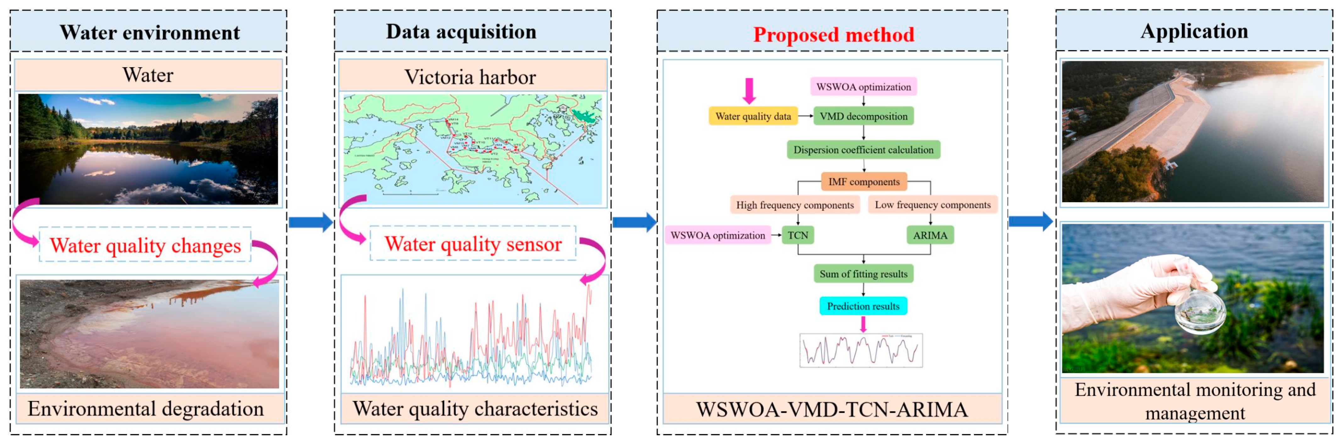
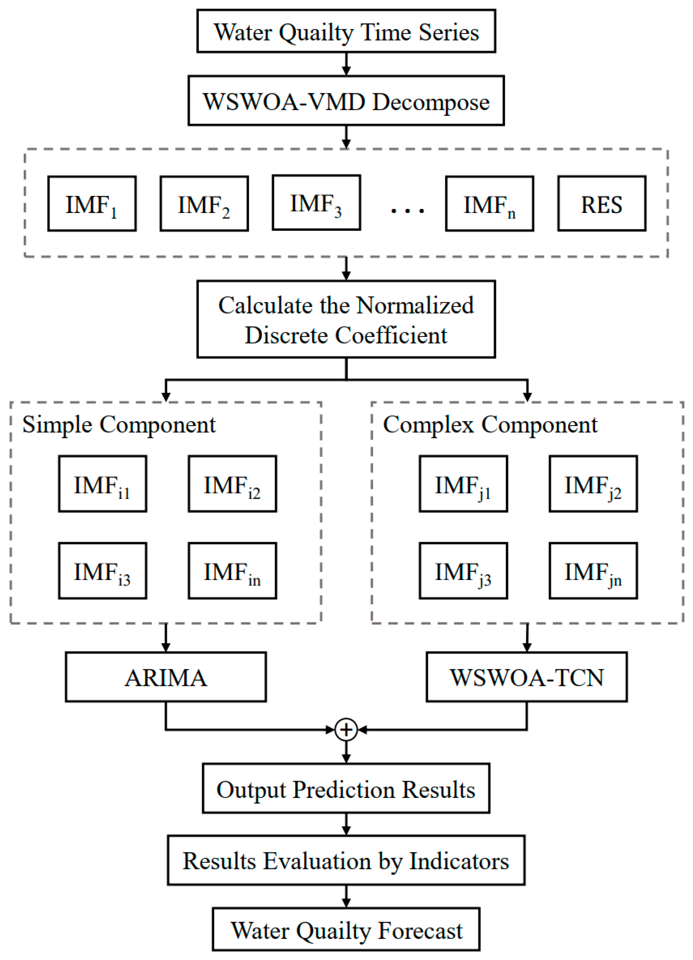
• The adaptive algorithm WSWOA-VMD is used to process water quality data. The number of modes and penalty parameters of VMD decomposition are optimized through WSWOA to improve the input quality of the prediction model.
• A TCN-ARIMA combination model is proposed to achieve water quality prediction. The different types of modal components obtained via decomposition are input into the corresponding prediction algorithms, which improves the accuracy and efficiency of the model.

The rest of this paper is constructed as follows. In Section 2, the method used in this article and the established framework are described, including parameter optimization, feature extraction and combined prediction modules. Section 3 takes the Victoria Harbor VM1 monitoring station data as an example for prediction and shows the prediction results. Section 4 analyzes the prediction results to verify the superiority of the prediction results. Section 5 is a discussion of the results of this study. Finally, the conclusions are drawn in Section 6. The flowchart of this work is shown as Figure 1.

2. Methodology

2.1. Parameter Optimization Model

2.1.1. WOA

In 2016, Mirjalili et al. [27] proposed the WOA algorithm, a bionic meta-heuristic optimization algorithm based on the feeding behavior of humpback whales in nature. Due to its high global search capability and rapid convergence speed in solving the optimization of model parameters, the WOA has a wide range of application scenarios. The algorithm consists primarily of three components: encircling prey, bubble net fishing, and random search. The specific steps are as follows:

• Step 1: Encircling prey

Each whale in the WOA represents an individual, the individual’s position in the search space represents the solution, and the individual’s search range is the solution space. When a group of whales hunts prey, they must establish the location of the prey and encircle it, assuming that the optimal solution in the current population is the target prey or the location closest to the prey, and the other individual whales in the population continue to approach the optimal solution. The expression of this behavior is as follows:

$$D =\left|{C·X}^{*}\left(t\right)-X_i\left(t\right)\right|,$$

(1)

$$X_i\left(t+1\right){=X}^{*}\left(t\right)-A·D.$$

(2)

where t is the current iteration, $X_i\left(t\right)$ denotes the position of individual i in the population at moment t, $X^{*}\left(t\right)$ denotes the current optimal position vector. The coefficients of variation A and C are calculated as follows:

$$A=2a·r-a,$$

(3)

$$C=2r,$$

(4)

where $a$ is a linearly decreasing contraction factor from 2 to 0 and $r$ is a random value in the range [0, 1].

• Step 2: Bubble net fishing

The variable coefficient A and C largely determines the updating of the position of the captured prey, as shown by the preceding equation. However, the bubble net feeding mechanism, which reproduces a hunting method unique to humpback whales, is accomplished by creating bubbles in paths similar to the number 9. The majority of its position update is determined by the spiral logarithmic equation with the expression:

$$X_i\left(t+1\right){=D}^{‘}{\times e}^{bl}\times \cos \left(2\pi l\right){+X}^{*}\left(t\right),$$

(5)

$$D^{‘}=\left|X^{*}\left(t\right)-{ X}_i\left(t\right)\right|,$$

(6)

where $b$ is a logarithmic helix constant to control the shape of the helix and $l$ is a random number in [−1, 1].

In addition, while whale populations engage in predation, they move towards the location of their prey using a round-up prey mechanism and a bubble net predation mechanism, with the WOA selecting the mechanism to move based on the probability p, which is chosen as shown below:

$$X_i\left(t+1\right)=\left\{\begin{array}{cc}{X}^{*}\left(t\right)-A·D \hfill & \hfill p < 0.5\hfill \\ D^{‘}{ \times e}^{bl}\times \cos \left(2\pi l\right){+X}^{*}\left(t\right) \hfill & \hfill p \ge 0.5\hfill \end{array}\right..$$

(7)

• Step 3: Random search

To investigate all solutions in the searchable space. According to the size of the absolute value of the variable coefficient A, the way of moving is judged. When |A| < 1, the individuals of the population move to the optimal position in the population through the mechanism of rounding up prey or the mechanism of bubble net predation; when |A| > 1, the individuals move randomly to expand the search range of the population and avoid the situation of locally optimal solutions, the expression is shown as follows:

$$D^{‘‘}=\left|{C·X}_{i,\mathit{rand}}-X_i\left(t\right)\right|,$$

(8)

$$X_i\left(t+1\right){=X}_{i,\mathit{rand}}-{A·D}^{‘‘},$$

(9)

where $X_{\mathit{rand}}$ is a randomly generated location.

The WOA is characterized by a strong global search capability and a fast convergence speed. However, the WOA only uses the optimal position in the population at the current moment and does not use the positional information of the individuals in the past moments, which restricts the range and direction of their individual movements. In addition, the combination of the position variable X and the distance variable D in the update of individual positions is relatively monotonous, reducing the diversity of the population. Therefore, the way of updating individual positions in the whale optimization algorithm needs to be updated.

2.1.2. WSWOA

The original WOA has restrictions on the mining and utilization of population data [28]. First, the combination of position variable X and distance variable D in the position update method of the WOA individual search does not make full use of their respective characteristics, and the relative importance of both should be altered during different periods to increase population diversity. In this study, we present the perturbation strategy of the double weighting factor, which modifies the weights of X and D based on two inversely varying parameters ${\omega }_1$ and ${\omega }_2$, which are calculated as follows:

$${\omega }_1=1 -\sin \left(\frac{\pi ·t}{2T}\right),$$

(10)

$${\omega }_2=1+\sin \left(\frac{\pi ·t}{2T}\right).$$

(11)

The double weighting factor improves the model’s ability to update individuals in the late population and can effectively prevent the model from reaching local optima. The improved update formulae for encircling prey, bubble net fishing, and random search are as follows:

• Encircling prey:

$$X_i\left(t+1\right){=\omega }_1{·X}^{*}\left(t\right)-{\omega }_2·A·D;$$

(12)

• Bubble net fishing:

$$X_i\left(t+1\right){=\omega }_1{·D}^{‘}{ \times e}^{\mathit{bl}} \times \cos \left(2\pi l\right){+\omega }_2{·X}^{*}\left(t\right);$$

(13)

• Random search:

$$X_i\left(t+1\right){=\omega }_1{·X}_{i,\mathit{rand}}-{\omega }_2{·A·D}^{‘‘}.$$

(14)

Secondly, the WOA does not mine and use historical positional information, limiting the direction and velocity of individual movement and the rate of population convergence. In this study, we refer to the individual updating method of particle swarm optimization combined with the perturbation strategy of double weight factor and add the following search method to the WOA:

$$X_i\left(t+1\right){=\omega }_1{·X}_i\left(t\right){+\omega }_2{·V}_i\left(t\right).$$

(15)

$$V_i\left(t\right){=V}_i\left(t-1\right){+r}_1\left(\mathit{ibest}-X_i\left(t-1\right)\right){+r}_2\left(\mathit{gbest}-X_i\left(t-1\right)\right),$$

(16)

where $X_i\left(t\right)$ and $V_i\left(t\right)$ represent the position and velocity of individual $i$ at moment $t$; $\mathit{ibest}$ is the best position experienced by the individual $I$; $\mathit{gbest}$ is the best position experienced by the population; and $r_1$ and $r_2$ are random numbers between 0 and 1.

As shown in Equations (12)–(16), the WSWOA algorithm continues to adhere to the humpback whale predation strategy, retaining the characteristics of robust global search capability and rapid convergence speed. However, the WSWOA introduces a double weighting factor and a new search strategy that can effectively use the information of both individuals and groups, improve the algorithm’s convergence speed, and enhance the capability of late population renewal.

2.2. Feature Extraction Model

2.2.1. VMD

The VMD is an adaptive, non-recursive variational modal algorithm that decomposes a signal into multiple local modal components [29]. These components, which are the oscillatory modes of the signal in distinct frequency ranges, can describe the volatility of the original signal. However, in contrast to EMD and CEEMAND, VMD needs to set the component number K before the decomposition, which related to the data decomposition effect directly [30]. These local modal components are defined as follows:

$$u_k\left(t\right){=A}_k\left(t\right){ \cos (\phi }_k\left(t\right)),$$

(17)

where t is the time, $A_k\left(t\right)$ is the signal envelope, and ${\phi }_k\left(t\right)$ is the signal’s instantaneous phase. The specific implementation steps of VMD decomposition are as follows:

Step 1: Calculate the analytical signal and one-sided spectrum of each modal function component through Hilbert transformation, translate the frequency band of the signal to the baseband, and finally, obtain the bandwidth of the modal function component by calculating the gradient norm of the demodulated signal, which can be expressed as follows:

$$\Vert {\partial }_t·\left\{\left[\delta \left(t\right)+\frac{j}{\pi t}\right]{·u}_k\left(t\right)\right\}{·e}^{-{j\omega }_{k}t}{\Vert }_2^2.$$

(18)

Step 2: The decomposition yields K modal components that, in addition to determining their respective center frequency and bandwidth parameters, must satisfy the condition that the sum of all the components’ bandwidths is minimal. The constraint model is stated as follows:

$$\left\{\begin{array}{c}\min \left\{{\displaystyle \sum }_{k=1}^K\Vert {\partial }_t·\left\{\left[\delta \left(t\right)+\frac{j}{\pi t}\right]{·u}_k\left(t\right)\right\}{·e}^{-{j\omega }_{k}t}{\Vert }_2^2\right\}\hfill \\ s.t. {\displaystyle \sum }_{k=1}^K{u}_k=f\left(t\right) \hfill \end{array}\right..$$

(19)

Step 3: By introducing the Lagrange multiplier λ and the second-order penalty factor α, the constrained problem is equivalent to an unconstrained problem. The augmented Lagrangian function is as follows:

$$L\left(\left\{u_k\right\},\left\{{\omega }_k\right\},\lambda \left(t\right)\right)=a{{\displaystyle \sum }}_{k=1}^K\Vert {\partial }_t·\left\{\left[\delta \left(t\right)+\frac{j}{\pi t}\right]{·u}_k\left(t\right)\right\}{·e}^{-{j\omega }_{k}t}{\Vert }_2^2+\Vert f\left(t\right)-u_k\left(t\right){\Vert }_2^2+[\lambda \left(t\right),f\left(t\right)-{{\displaystyle \sum }}_{k=1}^K{u}_k\left(t\right)].$$

(20)

Step 4: The center frequency of each component is searched through the alternating direction multiplier method ADMM, and k components with established center frequency and bandwidth parameters are obtained:

$${\omega }_k^{n+1}=\frac{{{\displaystyle \int }}_0^{\infty }\omega ·{\left|{\hat{u}}_k\left(\omega \right)\right|}^{2}d\omega }{{{\displaystyle \int }}_0^{\infty }{\left|{\hat{u}}_k\left(\omega \right)\right|}^{2}d\omega },$$

(21)

$${\hat{u}}_k^{n+1}\left(\omega \right)=\frac{\hat{f}\left(\omega \right) -{{\displaystyle \sum }}_{i\ne k}{\hat{u}}_i\left(\omega \right)+\frac{\hat{\lambda } \left(\omega \right)}{2}}{1+2\alpha ·{\left(\omega -{\omega }_k\right)}^2}.$$

(22)

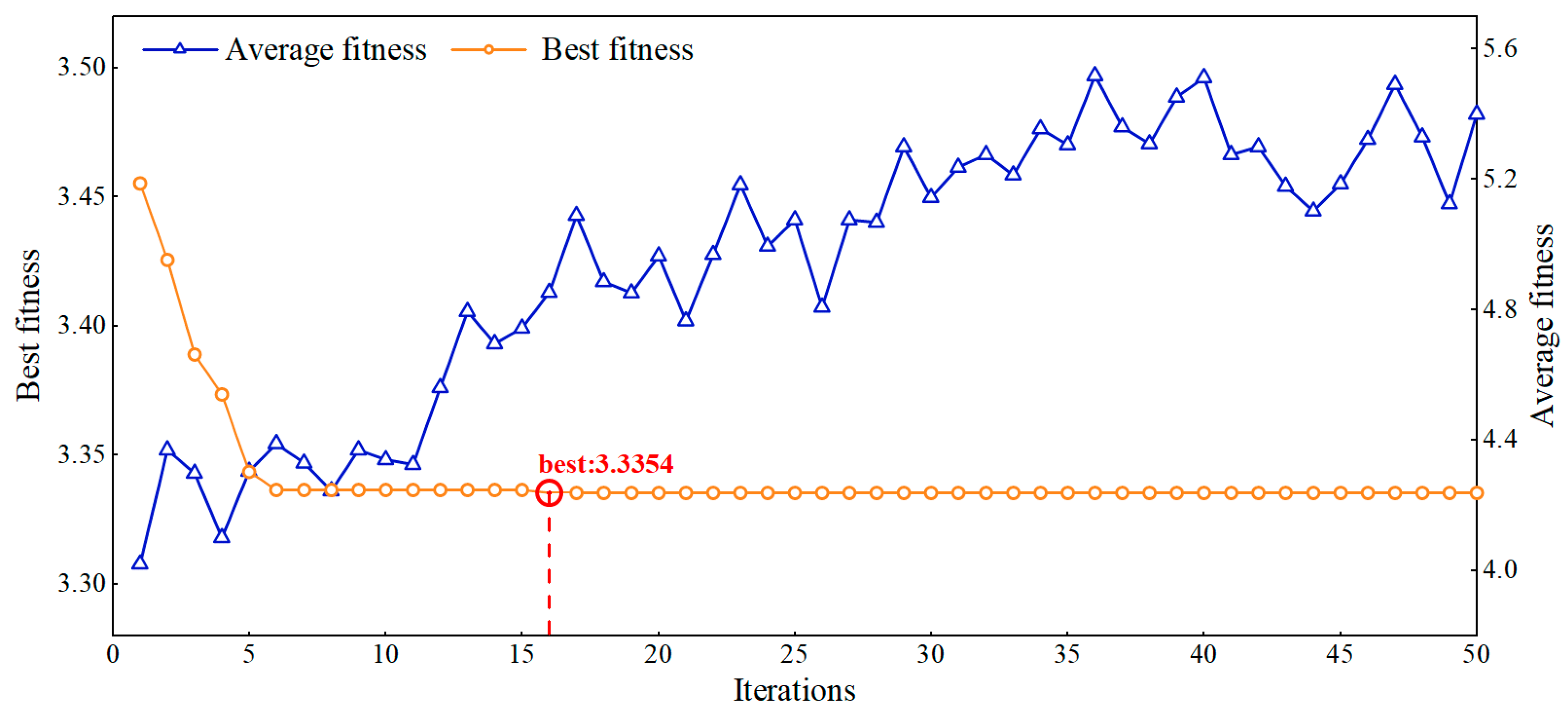
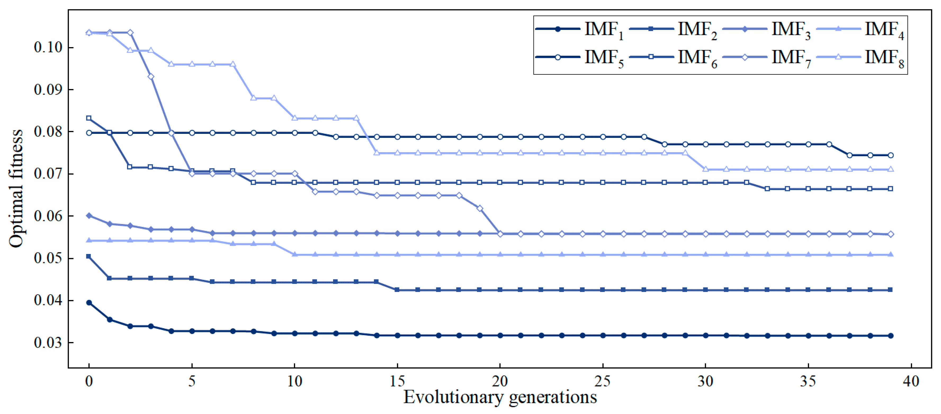
2.2.2. VMD Parameters Optimized Based on WSWOA

In the VMD decomposition procedure, the quadratic penalty factor $\sigma$ and the number of IMF components K must be manually specified. In the past, the settings of these parameters were frequently determined by the experimenter’s experience, which was largely a trial-and-error problem with large limitations. If the parameters are not chosen sensibly, the signal cannot be decomposed effectively, which impacts the data’s feature extraction and noise elimination [31]. Therefore, in order to obtain superior prediction results, it is necessary to choose appropriate $\sigma$ and K values for the VMD. In this paper, the WSWOA is selected to optimize the VMD to determine the optimal parameter combination [$\sigma$, K].

Permutation Entropy is a measure of entropy based on the theory of permutations that is primarily used to evaluate the randomness and complexity of signal sequences. It has been widely used in time series analysis [32]. In this study, the sum of the permutation entropy of each modal component is employed as its fitness function for parameter optimization of VMD decomposition. The calculation for the arrangement entropy is as follows:

Step 1: There is a time series data of length N: $\left\{X\left(i\right), i=1, 2,\dots ,N\right\}$, specifying an embedding dimension m and a time delay L, then reconstructing the original sequence space as $x$, with each subsequence denoted by $x\left(s\right)=X\left(s\right),X(s+L),\dots ,X[s+(m-1)\ast L]$. The expression after spatial reconstruction is as follows:

$$x =\left[\begin{array}{c}x\left(1\right)\\ x\left(2\right)\\ x\left(s\right)\\ \dots \\ x\left(k\right)\end{array}\right]=\left[\begin{array}{c}X\left(1\right) X\left(1+L\right) \dots X [1+\left(m-1\right)\ast L]\\ X\left(2\right) X\left(2+L\right) \dots X [2+\left(m-1\right)\ast L]\\ X\left(s\right) X\left(s+L\right) \dots X[s+\left(m-1\right)\ast L]\\ \dots \\ X\left(k\right) X\left(k+L\right) \dots X[k+\left(m-1\right)\ast L]\end{array}\right],$$

(23)

where the number of sequences k is calculated based on the embedding dimension m and the time delay $L$: $k=N-(m-1)\ast L$.

Step 2: Sorting incrementally the interior of each subsequence x(s) into $X[s+\left(z_m-1\right)\ast L]$, and recording its index $z_m$ in an ascending order as follows:

$${S\left(\xi \right)=(z}_1{,z}_2{,z}_3{,\dots z}_m), \xi =1, 2, 3,\dots ,\vartheta (\vartheta \le m!).$$

(24)

From Equation (24), it can be seen that $x\left(s\right)$ is mapped to $S\left(\xi \right)$ through incrementally sorting and index records. Thus, each $S\left(\xi \right)$ is one of the m! permutations.

Step 3: Calculate the probability of occurrence of different arrangements in all $S\left(\xi \right)$, denoted as $P_{\vartheta }$. Then, the permutation entropy calculation formula of time series $X\left(i\right)$ is as follows:

$$P_{ }={{\displaystyle \sum }}_{k=1}^K{P}_i{\ast \mathrm{lnP}}_i.$$

(25)

2.3. Combined Forecasting Model

2.3.1. Feature Classification

After the raw data are decomposed by the VMD, the degree of fluctuation of each IMF is different. To ensure the accuracy of the model and at the same time minimize the time consumption of prediction, we differentiate between complex and simple components by calculating the standardized discrete coefficients of each IMF. Then, the complex components are fed into a deep network that requires extensive training time for fitting, while the simple components are fed into a regression model that does not require extensive training time for fitting. The standardized discrete coefficient $c_v$ is calculated as follows:

$$C_v=\frac{\epsilon }{\mu },$$

(26)

$$c_v=\frac{C_v {- C}_v{}_{\min }}{C_v{}_{\max }-C_v{}_{\min }},$$

(27)

where $\epsilon$ is the standard deviation and $\mu$ is the mean.

2.3.2. Model Selection

To efficiently accommodate the variation of complex components, we require a deep learning model that can learn enough about the evolutionary characteristics of the time series. The TCN is an algorithm model for analyzing time series proposed by Shaojie Bai et al. in 2018 [33]. In contrast to the original CNN network, the TCN employs a causal convolution module and deforms the one-dimensional convolution to make the convolutional network appropriate for processing one-dimensional time series data. In addition, the extended convolution module and residual portions are added to the model to implement its memory function. A brief description of each structure follows.

The TCN network is based on the convolutional network architecture to deal with time series data, with causal convolution, extended convolution, and residuals as its three primary modules. As shown in Figure 2a, causal convolution is a rigorously time-constrained model; the inputs at the current time can only depend on the input information prior to the current time, effectively avoiding the interference of future information. Whereas extended convolution, as shown in Figure 2b, is performed by skipping some of the inputs, allowing the deep network to learn a wider range of inputs and avoiding the problem of excessive network depth and vanishing gradients due to learning more inputs.

Blindly stacking convolutional layers can lead to issues with vanishing gradients, explosions, and degradation, even when causal and extended convolution are applied [34]. Therefore, the TCN network employs a residual block module, which has been proven to be an effective method for training deep networks, allowing the network to transfer information between layers [35]. Its structure is shown in Figure 3. The residual block is composed of two sets of extended causal convolutional layers, a weight normalization layer, a nonlinear mapping function called Relu, and a Dropout layer.

To fit the simple features quickly and accurately, the integrated autoregressive average moving average model was chosen to fit the simple features in this study. ARIMA consists of three components—autoregressive (AR), differencing process (I), and moving average (MA)—and the algorithm can fit time series with minor fluctuations well [36]. It is ideally suited for forecasting simple components decomposed by the VMD. The mathematical model of the algorithm is as follows:

$${\hat{y}}_t={{\displaystyle \sum }}_{i=1}^p{\varphi }_i{y}_{t-i}{+\epsilon }_t-{{\displaystyle \sum }}_{j=1}^q{\theta }_j{\epsilon }_{t-j},$$

(28)

where ${\hat{y}}_t$ is the predicted value at moment t; $y_{t-i}$ is the real value at moment $t-I$; ${\theta }_j$ is the moving average term; ${\varphi }_i$ is the autoregressive term; ${\epsilon }_t$ is the random error; $p$ is the number of autoregressive parameters; and $q$ is the number of moving average parameters, which are determined by autocorrelation coefficients and bias correlation coefficients.

2.4. VMD-TCN-ARIMA Model Optimized by WSWOA

The overall process of the water quality characteristics prediction model is shown in Figure 4. First, in this study, the VMD decomposition algorithm is combined with the TCN and ARIMA, with the VMD decomposing and extracting features from the original time series data. Secondly, the IMF components were then classified by calculating standardized dispersion coefficients. Simple components are fed into the ARIMA for prediction and complex components are fed into the TCN for training and prediction. Finally, the parameters in the VMD and TCN are optimized by using the WSWOA proposed in the previous section to improve the accuracy of the model and reduce the consumption time of the model.

The specific steps of water quality prediction based on VMD-TCN-ARIMA optimized by WSWOA are shown below:

Step 1: Decomposing and reconstructing the original time series by the VMD, and the WSWOA algorithm is used to optimize the parameters of the VMD;

Step 2: Calculating the standardized dispersion coefficient of each IMF and classifying each component into two categories: complex and simple;

Step 3: Using the TCN to predict complex components and optimize the parameters of the TCN network through the WSWOA;

Step 4: Using the ARIMA to predict simple components;

Step 5: The output values of each IMF component are superimposed to finally generate the prediction results of water quality characteristics.

3. The Result of the Proposed Model

3.1. Dataset Settings

The design and analyses of this study are based on the historical dataset of various water quality indicators collected at the VM1 monitoring station in Victoria Harbour Bay, Hong Kong, which includes a total of 342 months of official statistics of various water quality indicators during the period from January 1992 to June 2020. Including dissolved oxygen (DO), dissolved oxygen saturation (DOsat), suspended solids (SS), salinity, pheophytin, lake transparency (SD), silica (SiO₂), biochemical oxygen consumption (BOD), total nitrogen (TN), a total of 10 water quality characteristics. The resolution of the dataset varied from semi-monthly to monthly, with each measurement including water quality levels at three depths: surface, middle, and bottom.

In this study, we selected data measured at the surface level, and we considered the effect of the data resolution on the prediction. We uniformly screened the data according to a resolution of one month and ultimately selected 342 data points from January 1992 to June 2020, of which 274 data points were used as a training set and 68 data points were used as a test set.

3.2. Evaluation Metrics

In order to objectively evaluate the performance and efficacy of an algorithm when time series are forecasted using a combined model, reasonable evaluation indices must be established to calculate the various categories of differences between the predicted and actual values produced by the model [37].

Four generally applicable metrics are chosen to evaluate the performance of the proposed prediction model. The formulae and brief descriptions are provided in

Table 1. Selection and interpretation of evaluation indicators.

Metrics	Formula	Explanation
RMSE (Root Mean Square Error)	$\sqrt{\frac{1}{N}{\displaystyle {\displaystyle \sum }_{i=1}^N}{\left(y_p{}^1-{ y}_t{}^2\right)}^2}$	RMSE denotes the mean error, which is more sensitive to extreme values, and it can be used as the benchmark for the robustness test of the model.
MAE (Mean Absolute Error)	$\frac{1}{N}{\displaystyle {\displaystyle \sum }_{i=1}^N}\left|y_p-y_t\right|$	MAE is a linear score in which all individual differences are equally weighted on the mean.
SMAPE (Symmetric Mean Absolute Percentage Error)	$\frac{100\%}{N}{\displaystyle {\displaystyle \sum }_{i=1}^N}\frac{\left|y_p-y_t\right|}{(\left|y_p\right|+\left|y_t\right|)/2}$	SMAPE uses a percentage 0–100% to represent the error size of the model.
NSE (Nash–Sutcliffeefficiency Coefficient)	$1-\frac{{{\displaystyle \sum }}_{i=1}^N{\left(y_p-y_t\right)}^2}{{{\displaystyle \sum }}_{i=1}^N{\left({\overline{y}}_t-{ y}_t\right)}^2}$	NSE is widely utilized model performance indices in the water-related research domain, and the closer the value is to 1, the better the predictive ability of the model.
R2 (Coefficient of Determination)	$\frac{{\left({{\displaystyle \sum }}_{i=1}^N\left({\overline{y}}_t-{ y}_t\right)\ast \left({\overline{y}}_p-{ y}_p\right)\right)}^2}{{{\displaystyle \sum }}_{i=1}^N{\left({\overline{y}}_t-y_t\right)}^2\ast {{\displaystyle \sum }}_{i=1}^N{\left({\overline{y}}_p-{ y}_p\right)}^2}$	R2 represents the goodness of model fitting. The closer the value is to 1, the better the fit between the fitted value and the actual value, and the better the model performance.

Notes: ¹ $y_p$ is the predicted value. ² $y_t$ is the true value.

.

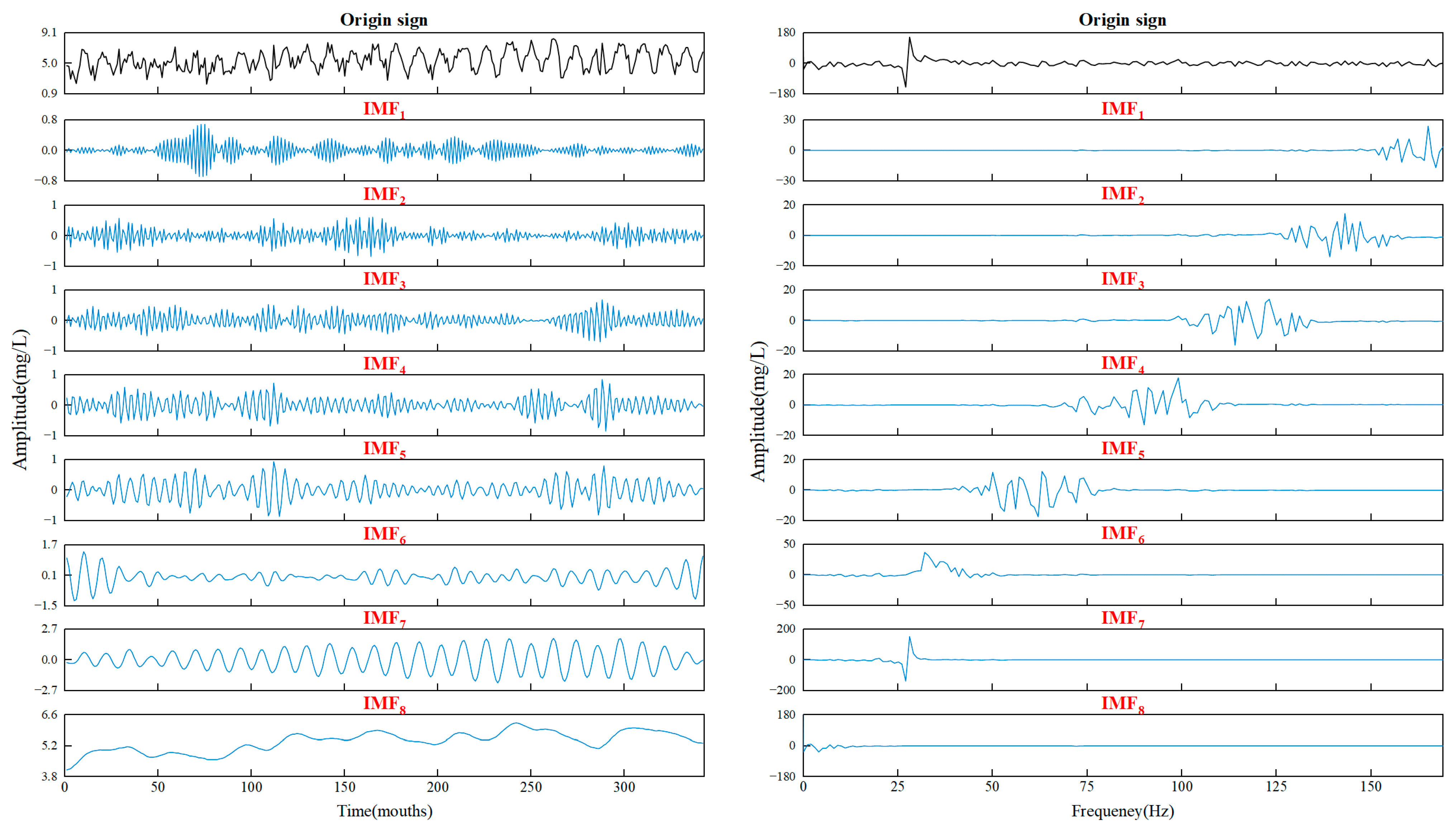
3.3. Model Decomposition Results Based on WSWOA-VMD

To reduce the impact of non-stationary and random noise in the original time series data on the prediction, the original data were decomposed using the VMD decomposition algorithm optimized through the WSWOA. The population size of WSWOA is set to 40, the maximum number of iterations is set to 40, the number of optimization variables is set to 2, the range of the penalty factor $\sigma$ is set to [1000, 9999], and the range of the decomposition number K is set to [4, 12], with all values being integers. Using DO data as an illustration, Figure 5 depicts the optimal fitness curve and the average fitness change curve during the iterative process of WSWOA.

As shown in Figure 5, the WSWOA reaches the optimal position after 16 iterations with an optimal fitness value of 3.3354, the optimal quadratic penalty factor $\sigma$ and the number of IMF components K as 1307 and 8, respectively. According to the changes in the average fitness curves, it can be inferred that the model does not fall into local search local search during the later stages of iteration, and effectively prevented it from converging to a local optimum.

Figure 6 shows the time and frequency domain plots of each modal component after VMD decomposition based on the optimal parameters. According to the spectrograms, the individual modes are independent of one another, effectively avoiding the issue of modal blending and demonstrating the viability of WSWOA-VMD.

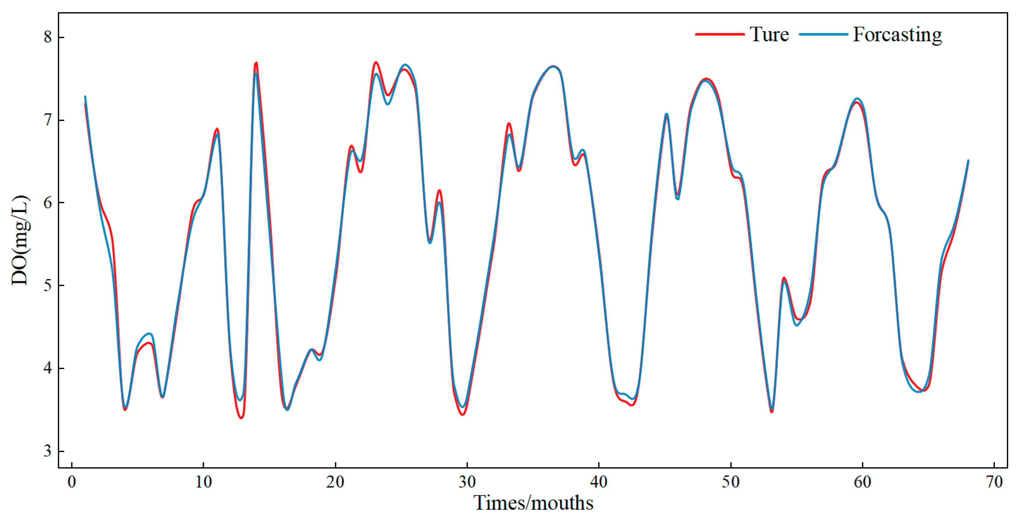
3.4. Water Quality Prediction Results Based on WSWOA-VMD-TCN-ARIMA

The ARIMA and TCN are both algorithms for predicting time series, and the effect of the ARIMA is positively correlated with the regularity of the data. The TCN is a deep learning algorithm that can learn complex patterns of data change, but its training and prediction are slower than the ARIMA. Therefore, simple components are predicted with the ARIMA and complex components with the TCN, which can substantially improve the model’s speed and precision.

The time series forecasting model was the ARIMA-TCN combined model. First, the optimal parameters in the TCN are determined by the WSWOA. The population size is set to 40, the maximum number of iterations is set to 40, the number of variables is set to 2, the range of the learning rate LR is set to [0.001, 0.1], the range of the time step T is set to [4, 12] and only integer values are allowed, and the RMSE index after the prediction of the TCN is selected as the individual’s fitness function. Taking the 8 IMF components of DO as an example, WSWOA was employed to determine the optimal network parameters for each IMF component. Figure 7 demonstrates the optimal fitness curves for the TCN network parameters for the eight IMF components.

The parameter settings of the TCN network for the eight IMF components are shown in

Table 2. Optimal parameter parameters of TCN and categories for IMF component.

	Time Step T	Learning Rate LR	${\mathit{c}}_{\mathit{v}}$	Classification
IMF1	7	0.105	1.000	complex
IMF2	7	0.099	0.857	complex
IMF3	7	0.052	0.594	complex
IMF4	8	0.073	0.401	complex
IMF5	5	0.114	0.225	complex
IMF6	4	0.325	0.158	simple
IMF7	4	0.097	0.076	simple
IMF8	4	0.032	0.000	simple

. The individual IMF components were then classified as either complex or simple based on the magnitude of their respective standardized dispersion coefficients $c_v$ by establishing thresholds. In this study, a threshold value of 0.2 was established for the standardized dispersion coefficient; when it exceeded 0.2, the IMF component was judged to be a complex component and was input into the TCN for prediction, whereas it was judged to be a simple component and was input into the ARIMA for prediction when it was below 0.2. Table 2 shows the standardized dispersion coefficients and categories for the eight IMF components of the water quality characteristic DO.

The various categories of IMF components are input into the corresponding prediction models, and the prediction of our original series is obtained by summing all the predicted values. Figure 8 is the prediction result of water quality characteristic DO by this model.

The combined model VMD-TCN-ARIMA optimized by WSWOA proposed in this paper produces good fitting accuracy in the prediction of water quality characteristics DO and maintains good robustness in the face of fluctuating data, as shown in Figure 8. The evaluation metric NSE and R² of this prediction is 0.9951 and 0.9957, which is close to 1. The RMSE is 0.0958 mg/L, the MAE is 0.0747 mg/L, and the SAMPE is 1.48%.

4. Analysis of Experimental Results

4.1. Multi-Model Comparison

This study is a combined model to predict water quality, so in order to evaluate the predictive effectiveness of the model on water quality characteristics, two types of comparative tests were constructed to verify the strengths and weaknesses of each part of the model. The first category is to validate the efficacy of the WSWOA optimization algorithm on the model parameters, while the second category is to validate the efficacy of the VMD decomposition algorithm and the TCN-ARIMA combined prediction algorithm.

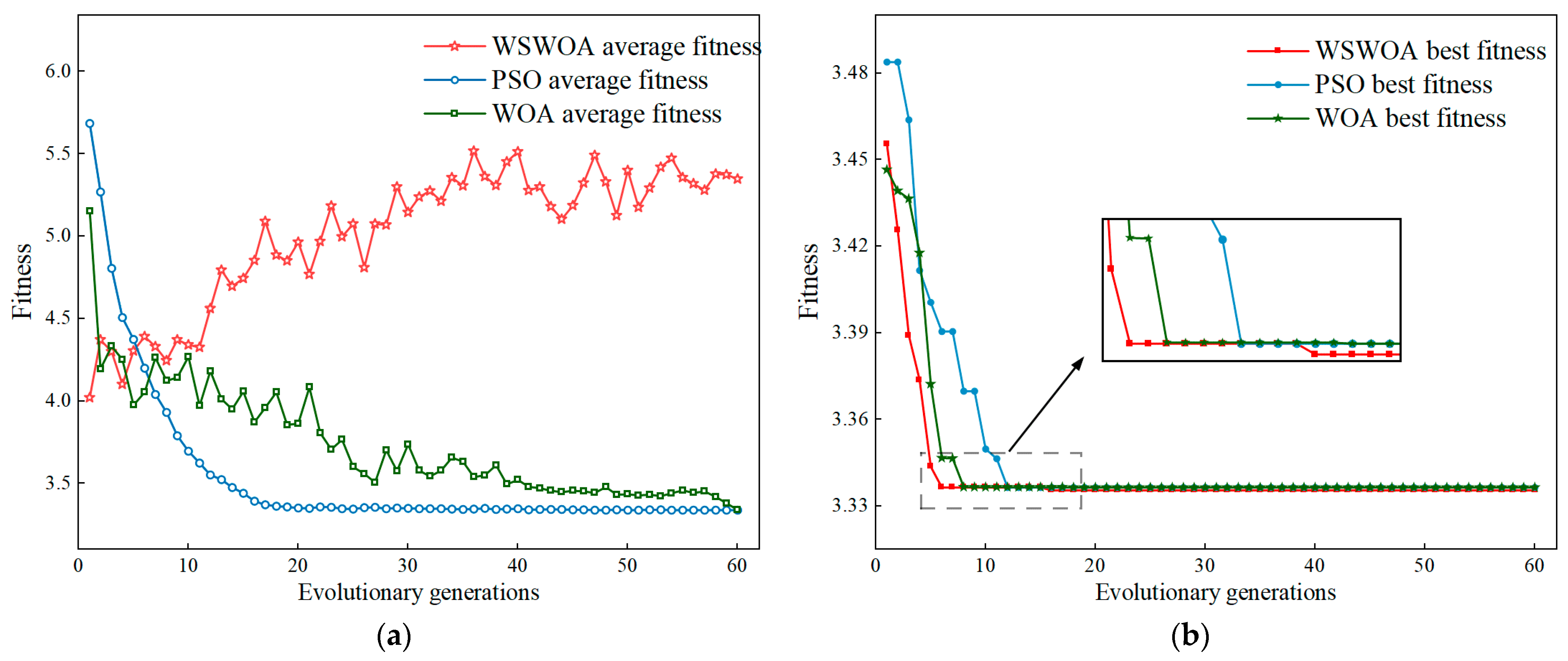
4.1.1. The Influence of Using Optimization Algorithm WSWOA

This study compares the variation of the fitness curves of the PSO and WOA in optimizing the parameters of the VMD for water quality characteristics DO. The parameter settings of the PSO and WOA algorithms are consistent with the WSWOA, the number of populations is set to 40, the maximum number of iterations is set to 40, the number of variables is set to 2, the range of penalty factor $\sigma$ is set to [1000, 9999], and the range of decomposition number K value is set to [4, 12]. The comparison of fitness curves is shown in Figure 9.

From Figure 9, it can be observed that the optimal fitness of the WOA and PSO is lower than that of the WSWOA, and the population average fitness of the WSWOA is higher than that of the other algorithms in the late iteration period, indicating that the WSWOA has a stronger searching ability in the late iteration period and is better able to jump out of the local optimal case due to the algorithm’s incorporation of the stochastic perturbation strategy of the coupling double. Meanwhile, the WSWOA converges to lower values than the WOA and PSO when the number of iterations is small. This is because the WSWOA combines PSO’s position updating method with WOA, which enhances the algorithm’s convergence performance. These two results demonstrate that the WSWOA can be used to optimize the VMD.

4.1.2. The Influence of Using Combined Model

In this study, ten additional models were constructed to validate the effect of adding the VMD data decomposition algorithm and the ARIMA prediction model. The compared models include BP, LSTM, TCN, ARIMA, VMD-TCN, EMD-TCN, CEEMDAM-TCN, and VMD-LSTM-ARIMA. To ensure that the variables underlying the comparison experiments were consistent, the BP, LSTM, TCN, and VMD algorithms in these models were optimized by WSWOA for the parameters, and the population size and number of iterations of the WSWOA algorithms were consistent with the model setups in this study. In addition, to compare with recent similar studies, this study adds the CEEMDAN-IWOA-BP model to verify the performance of the model. The prediction curves of all compared models are shown in Figure 10, and the evaluation metrics of the prediction results are shown in

Table 3. Comparison of evaluation metrics of the prediction results.

Model	Abbreviation	RMSE/mg	MAE/mg	SMAPE	NSE	R2	TIME
BP	#1	0.936	0.684	12.86%	0.518	0.723	1.89
LSTM	#2	0.890	0.675	12.61%	0.564	0.756	7.65
ARIMA	#3	1.139	0.843	15.32%	0.487	0.691	0.82
TCN	#4	0.872	0.629	11.98%	0.582	0.763	6.82
VMD-TCN	#5	0.163	0.121	2.39%	0.985	0.994	42.44
EMD-TCN	#6	0.495	0.372	7.31%	0.866	0.935	32.39
CEEMDAN-TCN	#7	0.572	0.426	8.47%	0.822	0.901	34.58
VMD-LSTM-ARIMA	#8	0.158	0.123	2.38%	0.986	0.994	44.42
VMD-TCN-ARIMA	#9	0.096	0.075	1.48%	0.995	0.996	31.38
CEEMDAN-IWOA-BP	#10	0.632	0.414	8.26%	0.828	0.911	11.96

.

• The influence of adding WSWOA-VMD

Compared with #4 and #5, the VMD decomposition conducts feature extraction and noise reduction on the original time series, resulting in reductions of 0.718, 0.508, and 9.59% in RMSE, MAE, and SMAPE, respectively. Simultaneously, it enhances NSE by 0.401 and R² by 0.231. According to the results, VMD decomposition of raw water quality sequences can provide enough effective information for the prediction model and substantially improve the prediction accuracy.

Compared with #5, #6, and #7, the currently commonly used time series decomposition algorithms EMD and CEEMDAN reduce NSE compared to the VMD for water quality time series data with large fluctuations and many influencing factors, respectively, 12.1% and 16.6%. This demonstrates that the VMD is significantly better than the EMD and CEEMDAN for predictive optimization of water quality data and is capable of good feature extraction and noise reduction of the original time series.

2.

The influence of using TCN-ARIMA

Compared with #1, #2, #3, and #4, it demonstrates that the TCN matches the water quality data better than the LSTM, BP, and ARIMA, thereby validating the selection of the TCN as the core prediction model. However, the ARIMA is significantly less time-consuming than deep networks that require training, and selecting the ARIMA can increase the prediction efficiency of the model.

Compared with #5, #8, and #9, the model with the highest NSE and the least time-consuming prediction is the model proposed in this study. Example #9 improves NSE by 0.9% and reduces time consumption by 26.1% compared to #5, indicating that adding ARIMA not only improves prediction efficiency but also reduces prediction errors and optimizes prediction accuracy #9 has a 0.9% improvement in NSE compared to #8, indicating that the prediction accuracy of TCN-ARIMA for the feature sequence after VMD decomposition is higher than that of LSTM-TCN. The model proposed in this study has stronger fitting capability for water quality data and can mine more time series information.

4.2. Further Research

To further verify the generalization ability of the proposed model, this study also predicted the remaining nine water quality characteristics of the proposed area. The settings of the optimization algorithm and the process of the prediction model were consistent with the water quality characteristic DO. The VMD decomposition parameters and evaluation indicators of prediction results for the nine water quality characteristics are shown in

Table 4. Evaluation metrics for prediction results of other water quality characteristics.

	VMD Optimal Solutions		RMSE	MAE	SMAPE	NSE	R2
	K	σ
DOsat	9	1190	1.467	1.146	1.40%	0.985	0.994
SS	8	1277	0.436	0.349	8.17%	0.987	0.994
turbidity	8	1013	0.293	0.239	9.55%	0.988	0.995
Salinity	9	2082	0.185	0.146	0.48%	0.989	0.996
Pheophytin	7	1761	0.113	0.092	13.09%	0.986	0.995
SD	9	1311	0.098	0.072	3.02%	0.980	0.994
SiO2	9	1769	0.041	0.032	6.09%	0.985	0.995
BOD	9	1569	0.033	0.027	7.66%	0.985	0.993
TN	9	1149	0.023	0.019	5.51%	0.983	0.993

.

It can be seen from Table 4 that the evaluation metric NSEs of the remaining nine water quality characteristics are all above 0.98, indicating that this model can learn the change patterns of different water quality characteristics and predict them effectively. It is demonstrated that the WSWOA-VMD-TCN-ARIMA water quality prediction model proposed in this study has a very superior generalization ability to adaptively fit and predict different water quality characteristics.

5. Discussion

The experimental results in this study offer valid evidence for the effectiveness of the proposed WSWOA-VMD-TCN-ARIMA water quality predication model. First, in the assessment of the impact of the WSWOA optimization algorithm on VMD parameters, it is evident that WSWOA exhibits a pronounced superiority in convergence speed and late-stage search capabilities over PSO and WOA. This highlights its potential to effectively optimize model parameters. Second, the effectiveness of the VMD-TCN-ARIMA composite model is demonstrated through a comparison with ten similar models. The performance of WSWOA-optimized VMD surpasses that of EMD and CEEMDAN, showcasing its robust feature extraction and denoising capabilities for water quality time series data. The combined prediction method of TCN and ARIMA enables the proposed model to further improve the prediction accuracy and reduce the time consumption Finally, to validate the model’s generalization capability, predictions were extended to nine additional water quality characteristics. Across diverse features, the sustained high NSE values substantiate the model’s adaptive ability to forecast different water quality parameters. This underscores the outstanding generalization capability of the WSWOA-VMD-TCN-ARIMA model.

However, despite the proposed model exhibiting commendable performance in various, it is imperative to acknowledge certain limitations, warranting further investigation in the field of water quality prediction. For example, this study excluded external factors other than water quality data when predicting water quality. As the trends in water quality data are influenced by external variables, especially variables related to environmental changes such as weather and temperature, integrating these pertinent variables into water quality predictions would enable a more comprehensive understanding of the variations in water quality characteristics.

Therefore, in future water quality prediction studies, we should integrate external factors such as weather and temperature into prediction models to capture the subtle interactions between these variables and water quality dynamics. Secondly, current research generally focuses on improving model accuracy, and not many studies have focused on reducing model time consumption and improving prediction efficiency. In the future, more advanced optimization algorithms, innovative decomposition technologies, and accurate and rapid prediction models can be integrated to improve the accuracy and timeliness of predictions. Through these endeavors, the scientific community can propel research in water quality prediction to new heights, offering valuable insights for sustainable water resource management and environmental conservation.

6. Conclusions

In this study, we combined the VMD decomposition with the TCN network and the ARIMA regression model, and we used the WSWOA algorithm to optimize the parameters of the VMD and TCN to develop a combined VMD-TCN-ARIMA prediction model optimized by WSWOA. This model was then applied to the time series data of water quality characteristics from the monitoring stations in Victoria, Hong Kong. After comparing the proposed method with several existing water quality sequence prediction methods, our conclusions are as follows:

• The results of decomposing the time series demonstrate that the VMD optimized by WSWOA can effectively suppress the mixing of modal components, extract various features from the original sequence, and enhance the accuracy of the subsequent prediction steps. Compared with other existing parameter optimization algorithms, this method has stronger global search capabilities and faster convergence speed, providing an effective new method for existing model parameter optimization technology.
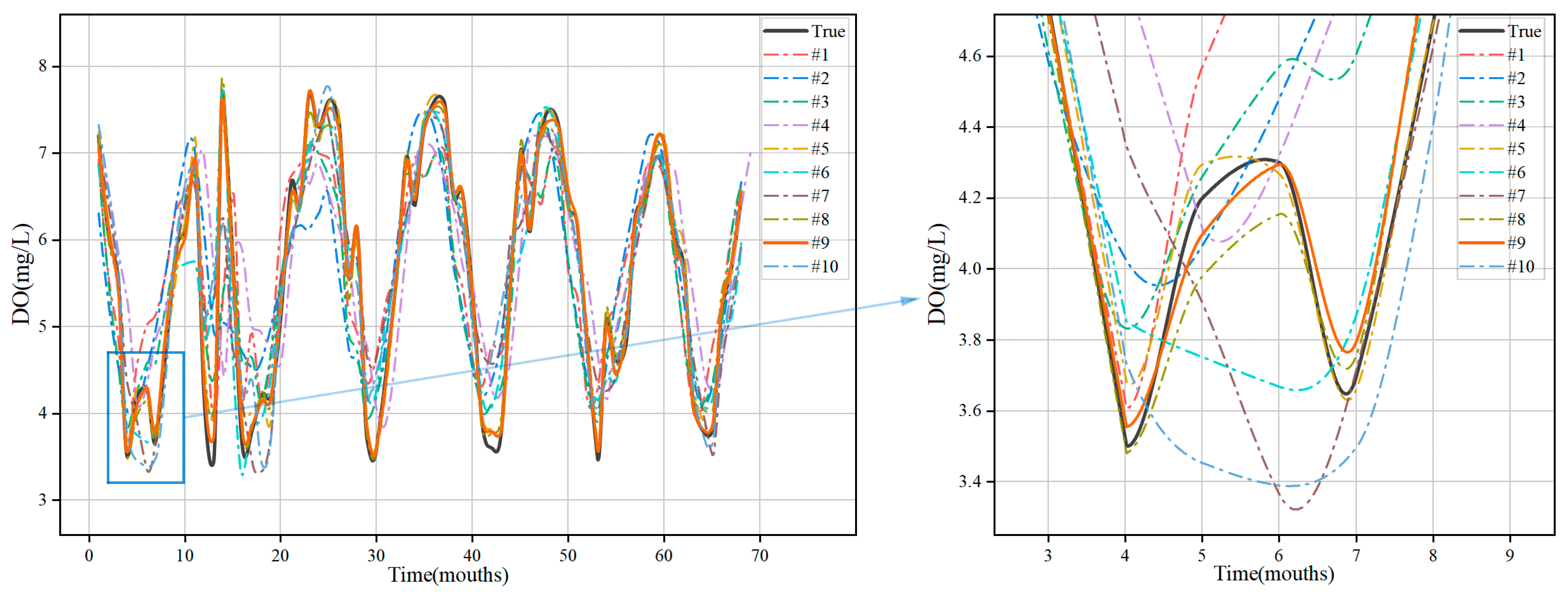
• Comparisons with different forecasting models show that the combined model is more accurate and efficient in forecasting than a single model. It is demonstrated that the TCN-ARIMA combined model can effectively suit the modal components following VMD decomposition of the original data and achieve more precise and faster prediction results.
• The results of predicting multiple water quality characteristics demonstrate that the model in this study is distinct from the majority of models at this stage, which must be restricted to a fixed range of water quality areas and characteristics. The model proposed in this study can adaptively find the optimal model parameters for different types of time series data by utilizing the WSWOA, which removes the need for manual adjustments and greatly improves the generalizability and intelligence of the model.

References

1. Shen, Z.X.; Zhang, Q.; Singh, V.P.; Pokhrel, Y.; Li, J.P.; Xu, C.Y.; Wu, W.H. Drying in the low-latitude Atlantic Ocean contributed to terrestrial water storage depletion across Eurasia. Nat. Commun. 2022, 13, 10. [Google Scholar] [CrossRef]
2. Yan, T.; Shen, S.-L.; Zhou, A. Indices and models of surface water quality assessment: Review and perspectives. Environ. Pollut. 2022, 308, 119611. [Google Scholar] [CrossRef] [PubMed]
3. Li, H.M.; Wang, F.Q.; Zhang, C.Y.; Wang, L.Y.; An, X.W.; Dong, G.H. Sustainable supplier selection for water environment treatment public-private partnership projects. J. Clean. Prod. 2021, 324, 18. [Google Scholar] [CrossRef]
4. Han, M.; Su, Z.Y.; Na, X.D. Predict water quality using an improved deep learning method based on spatiotemporal feature correlated: A case study of the Tanghe Reservoir in China. Stoch. Environ. Res. Risk Assess. 2023, 37, 2563–2575. [Google Scholar] [CrossRef]
5. Li, H.M.; Xia, Q.; Wen, S.P.; Wang, L.Y.; Lv, L.L. Identifying Factors Affecting the Sustainability of Water Environment Treatment Public-Private Partnership Projects. Adv. Civ. Eng. 2019, 2019, 15. [Google Scholar] [CrossRef]
6. Uddin, M.G.; Nash, S.; Rahman, A.; Olbert, A.I. A comprehensive method for improvement of water quality index (WQI) models for coastal water quality assessment. Water Res. 2022, 219, 20. [Google Scholar] [CrossRef]
7. Dong, Y.A.; Ren, Z.; Li, L.H. Forecast of Water Structure Based on GM (1,1) of the Gray System. Sci. Program. 2022, 2022, 7. [Google Scholar] [CrossRef]
8. Zhang, J.P.; Wang, Y.H.; Zhao, Y.; Fang, H.Y. Multi-scale flood prediction based on GM (1,2)-fuzzy weighted Markov and wavelet analysis. J. Water Clim. Chang. 2021, 12, 2217–2231. [Google Scholar] [CrossRef]
9. Ghaemi, E.; Tabesh, M.; Nazif, S. Improving the ARIMA Model Prediction for Water Quality Parameters of Urban Water Distribution Networks (Case Study: CANARY Dataset). Int. J. Environ. Res. 2022, 16, 10. [Google Scholar] [CrossRef]
10. Doorn, N. Artificial intelligence in the water domain: Opportunities for responsible use. Sci. Total Environ. 2021, 755, 10. [Google Scholar] [CrossRef]
11. Noori, R.; Karbassi, A.R.; Ashrafi, K.; Ardestani, M.; Mehrdadi, N. Development and application of reduced-order neural network model based on proper orthogonal decomposition for BOD5 monitoring: Active and online prediction. Environ. Prog. Sustain. Energy 2013, 32, 120–127. [Google Scholar] [CrossRef]
12. Chen, L.H.; Li, L. Evaluation of dissolved oxygen in water by artificial neural network and sample optimization. J. Cent. South Univ. Technol. 2008, 15, 416–420. [Google Scholar] [CrossRef]
13. AlDahoul, N.; Essam, Y.; Kumar, P.; Ahmed, A.N.; Sherif, M.; Sefelnasr, A.; Elshafie, A. Suspended sediment load prediction using long short-term memory neural network. Sci. Rep. 2021, 11, 22. [Google Scholar] [CrossRef]
14. Fu, Y.X.; Hu, Z.H.; Zhao, Y.C.; Huang, M.X. A Long-Term Water Quality Prediction Method Based on the Temporal Convolutional Network in Smart Mariculture. Water 2021, 13, 2907. [Google Scholar] [CrossRef]
15. Alizadeh, M.J.; Kavianpour, M.R. Development of wavelet-ANN models to predict water quality parameters in Hilo Bay, Pacific Ocean. Mar. Pollut. Bull. 2015, 98, 171–178. [Google Scholar] [CrossRef] [PubMed]
16. Noori, R.; Karbassi, A.; Ashrafi, K.; Ardestani, M.; Mehrdadi, N.; Nabi Bidhendi, G.-R. Active and online prediction of BOD5 in river systems using reduced-order support vector machine. Environ. Earth Sci. 2012, 67, 141–149. [Google Scholar] [CrossRef]
17. Li, L.; Liu, Y.J.; Wang, K.; Zhang, D. Simulation of Pollution Load at Basin Scale Based on LSTM-BP Spatiotemporal Combination Model. Water 2021, 13, 516. [Google Scholar] [CrossRef]
18. Baek, S.S.; Pyo, J.; Chun, J.A. Prediction of Water Level and Water Quality Using a CNN-LSTM Combined Deep Learning Approach. Water 2020, 12, 3399. [Google Scholar] [CrossRef]
19. Li, S.X.; Xie, J.C.; Yang, X.; Jing, X. Comparison of hybrid machine learning models to predict short-term meteorological drought in Guanzhong region, China. Water Sci. Technol. 2023, 87, 2756–2775. [Google Scholar] [CrossRef]
20. Zhang, Y.T.; Li, C.L.; Jiang, Y.Q.; Sun, L.; Zhao, R.B.; Yan, K.F.; Wang, W.H. Accurate prediction of water quality in urban drainage network with integrated EMD-LSTM model. J. Clean. Prod. 2022, 354, 12. [Google Scholar] [CrossRef]
21. Wang, F.H.; Zhang, D.M.; Min, G.Y.; Li, J.X. Reservoir Production Prediction Based on Variational Mode Decomposition and Gated Recurrent Unit Networks. IEEE Access 2021, 9, 53317–53325. [Google Scholar] [CrossRef]
22. Geng, G.C.; He, Y.; Zhang, J.; Qin, T.X.; Yang, B. Short-Term Power Load Forecasting Based on PSO-Optimized VMD-TCN-Attention Mechanism. Energies 2023, 16, 4616. [Google Scholar] [CrossRef]
23. Liu, F.P.; Liu, Y.; Yang, C.; Lai, R.X. A New Precipitation Prediction Method Based on CEEMDAN-IWOA-BP Coupling. Water Resour. Manag. 2022, 36, 4785–4797. [Google Scholar] [CrossRef]
24. Yan, T.; Zhou, A.N.; Shen, S.L. Prediction of long-term water quality using machine learning enhanced by Bayesian optimisation. Environ. Pollut. 2023, 318, 10. [Google Scholar] [CrossRef] [PubMed]
25. Flores, V.; Bravo, I.; Saavedra, M. Water Quality Classification and Machine Learning Model for Predicting Water Quality Status-A Study on Loa River Located in an Extremely Arid Environment: Atacama Desert. Water 2023, 15, 2868. [Google Scholar] [CrossRef]
26. Kumar, Y.; Kaur, A. Variants of bat algorithm for solving partitional clustering problems. Eng. Comput. 2022, 38, 1973–1999. [Google Scholar] [CrossRef]
27. Mirjalili, S.; Lewis, A. The Whale Optimization Algorithm. Adv. Eng. Softw. 2016, 95, 51–67. [Google Scholar] [CrossRef]
28. Lu, K.Z.; Ma, Z.M. A modified whale optimization algorithm for parameter estimation of software reliability growth models. J. Algorithms Comput. Technol. 2021, 15, 14. [Google Scholar] [CrossRef]
29. Zhang, Y.G.; Pan, G.F.; Chen, B.; Han, J.Y.; Zhao, Y.; Zhang, C.H. Short-term wind speed prediction model based on GA-ANN improved by VMD. Renew. Energy 2020, 156, 1373–1388. [Google Scholar] [CrossRef]
30. Noori, R.; Safavi, S.; Nateghi Shahrokni, S.A. A reduced-order adaptive neuro-fuzzy inference system model as a software sensor for rapid estimation of five-day biochemical oxygen demand. J. Hydrol. 2013, 495, 175–185. [Google Scholar] [CrossRef]
31. Wang, L.S.; Liu, Y.H.; Li, T.S.; Xie, X.Z.; Chang, C.M. Short-Term PV Power Prediction Based on Optimized VMD and LSTM. IEEE Access 2020, 8, 165849–165862. [Google Scholar] [CrossRef]
32. Rajabi, S.; Azari, M.S.; Santini, S.; Flammini, F. Fault diagnosis in industrial rotating equipment based on permutation entropy, signal processing and multi-output neuro-fuzzy classifier. Expert Syst. Appl. 2022, 206, 16. [Google Scholar] [CrossRef]
33. Lea, C.; Flynn, M.D.; Vidal, R.; Reiter, A.; Hager, G.D. IEEE. Temporal Convolutional Networks for Action Segmentation and Detection. In Proceedings of the 30th IEEE/CVF Conference on Computer Vision and Pattern Recognition (CVPR), Honolulu, HI, USA, 21–26 July 2017; pp. 1003–1012. [Google Scholar] [CrossRef]
34. Liu, X.L.; Zhao, J.J.; Lin, S.F.; Li, J.Q.; Wang, S.H.; Zhang, Y.M.; Gao, Y.Y.; Chai, J.C. Fine-Grained Individual Air Quality Index (IAQI) Prediction Based on Spatial-Temporal Causal Convolution Network: A Case Study of Shanghai. Atmosphere 2022, 13, 959. [Google Scholar] [CrossRef]
35. Song, T.Z.; Song, Y.; Wang, Y.X.; Huang, X.G. Residual network with dense block. J. Electron. Imaging 2018, 27, 9. [Google Scholar] [CrossRef]
36. Chodakowska, E.; Nazarko, J.; Nazarko, L.; Rabayah, H.S.; Abendeh, R.M.; Alawneh, R. ARIMA Models in Solar Radiation Forecasting in Different Geographic Locations. Energies 2023, 16, 5029. [Google Scholar] [CrossRef]
37. Han, Z.Y.; Zhao, J.; Leung, H.; Ma, A.; Wang, W. A Review of Deep Learning Models for Time Series Prediction. IEEE Sens. J. 2021, 21, 7833–7848. [Google Scholar] [CrossRef]
Figure 1. Flowchart of this work.
Water 15 04227 g001
Figure 2. Construction of TCN: (a) form of causal convolution; (b) form of extended convolution.
Water 15 04227 g002
Figure 3. Form of residual block.
Water 15 04227 g003
Figure 4. Flowchart of water quality prediction model.
Water 15 04227 g004
Figure 5. Fitness curve of VMD training process.
Water 15 04227 g005
Figure 6. Time domain waveform and spectrum diagram of water quality data decomposed by WSWOA-VMD.
Water 15 04227 g006
Figure 7. The optimal fitness curve of the TCN parameters of the IMF component.
Water 15 04227 g007
Figure 8. The optimal fitness curve of the TCN parameters of the IMF component.
Water 15 04227 g008
Figure 9. Optimal fitness and average fitness curves of different algorithms: (a) curves of average fitness; (b) curves of optimal fitness.
Water 15 04227 g009
Figure 10. Comparison of the prediction curves of multiple models.
Water 15 04227 g010