Waterborne Disease Risk Assessment and Mapping for a Floating Village by Combining 3D Hydraulic Simulation and Quantitative Microbial Risk Assessment

Abstract

Spatiotemporal changes in waterborne disease risk were evaluated for the Chhnok Tru floating village in the Tonle Sap Lake by combining a hydraulic simulation and quantitative microbial risk assessment (QMRA). First, a three-dimensional (3D) hydraulic simulation was performed, and the transport of Escherichia coli (E. coli) was simulated. Prior to the simulation, by coupling satellite imagery analysis using the normalized difference water index (NDWI) and a sounding survey using an acoustic Doppler current profiler (ADCP), a new digital elevation model was generated for the complex channel network with high resolution. The results of the 3D hydraulic simulation revealed the flow regime and nonuniform pathogen distribution in the floating village. QMRA was performed for the village using the E. coli distribution calculated by the 3D hydraulic model. Subsequently, the disease risk in the village was visualized through an effective and easy-to-understand disease risk map. To demonstrate the usefulness of the hydraulic-simulation-based disease risk map, the map was used to quantitatively compare simple policies by evaluating their reduction in disease risk.

1. Introduction

Tonle Sap Lake (TSL) is the largest freshwater lake in Southeast Asia, located approximately in the center of the Kingdom of Cambodia (Figure 1). Eleven major tributaries flow into the TSL, and the TSL is connected to the Mekong River (MR) through the Tonle Sap River (TSR) located southeast of the lake. The TSL has unique hydraulic and hydrological characteristics. The climate of the region is characterized by a clearly divided dry season (November to April) and wet season (May to October) [1].

During the dry season, the TSL releases a large amount of water into the MR through the TSR. In November, which is the beginning of the dry season, the TSL starts releasing water into the MR with a discharge of approximately 10,000 m${}^3$/s, which is the maximum discharge in the dry season. As a result, the water level in the TSL continuously decreases over time. In February, the release of water from TSL into MR weakens to a discharge of approximately 1000 m${}^3$/s. Then, for the next 3 months, until early May, the TSL maintains a shallow depth, with a minimum monthly depth of 1.5 m [2,3].

Conversely, during the wet season, the TSL receives a large amount of water from the MR due to reversal flow in the TSR [4]. The maximum flux of the reversal flow reaches approximately 10,000 m${}^3$/s. This phenomenon causes a significant rise in the TSL’s water level, filling up wide floodplains surrounding the lake. By the end of the wet season, the lake’s depth reaches 10 m, and the water surface area expands sixfold (15,000 km${}^2$) compared to that of the dry season (2600 km${}^2$) [2]. Due to the cyclical expansion and shrinking of its water area throughout the year, the TSL is referred to as the “heart of Cambodia”.

In addition to its function as a detention reservoir for the Mekong Delta area [3], the TSL provides important infrastructure for society and the ecosystem. It provides the largest fishery in Cambodia, accounting for 70% of the protein consumed in the country [5]. The flooded forests, shrubs, grasslands, and agricultural fields in the floodplain provide habitats and food for a wide range of species, including globally threatened species. In addition, the lake provides not only economic infrastructure but also places of residence. More than one million people live in the TSL’s floodplain [6]. To cope with seasonal fluctuations in the water level, a large number of people live in floating houses (Figure 2), with ceramic pots or plastic drums fastened to the bases of the houses. Due to the buoyancy of the pots, the floating houses can continue to float on the water surface even as the water level of the lake changes. These floating houses cluster together and form communities, with approximately 90 villages in the TSL [7]. Figure 3 displays the Chhnok Tru floating village, which is one of the largest villages in the TSL and the target site of this study. The Chhnok Tru village is located along water channels in the transitional area connecting the TSL and TSR.

Although there is lake water under the thin floorboards of the houses, access to safe drinking water tends to be difficult, as public water supply pipelines do not reach the village. There are water stations where individuals can purchase lake water treated by filtration and chemical sterilization; however, the treated water is not affordable for a large number of households. Many households lack private land for farming and depend entirely on unstable fishing [8]. The majority of households are below the poverty line, suffering from severe poverty [9]. According to a recent baseline survey conducted using a questionnaire [10], approximately half of the residents of the village have consumed lake water, with approximately 30% of the water being untreated. Therefore, the residents are susceptible to infection of waterborne diseases due to use of unsafe water. However, there are hardly any sanitation facilities to prevent pathogens from being excreted into the lake water. As there are no water supply pipes, there is also no sewage drainage system installed in the village. Figure 2b displays a toilet used in a floating house. The most common type of toilet is a hole in the floor through which feces drop directly into the lake water without being collected in a bucket. Thus, the lake water is easily contaminated with harmful pathogens found in feces. In fact, according to the questionnaire survey [10], almost all adults living in the floating village experience diarrhea at least once a year, with 18.8% of them having experienced severe diarrhea in their lives. In addition to diarrhea, it has been suggested that a number of people suffer from diseases such as parasitic infections and gastroenteritis caused by Helicobacter pylori, which can be contracted through lake water contaminated by feces [11].

Knowing the flow regime is necessary for understanding the pathogen distribution trends in the village. Water currents carry away harmful lake water contaminated by pathogens; therefore, the concentration of pathogens in the lake water decreases over time. However, the actual reduction speed is expected to change according to the water flow state; high-speed flow quickly carries the pathogen to the outside of the village, and turbulent flow accelerates pathogen reduction by enhancing dilution with the surrounding clean water. Furthermore, water currents determine the maximum area in which the pathogens can exist, as certain pathogens, such as Escherichia coli (E. coli), cannot survive in lake water beyond a certain period of time.

Numerical hydraulic simulation is a powerful tool to determine the spatial structure of water flow. For example, Hashimoto et al. [12] simulated flooding in Dhaka city, Bangladesh, using a two-dimensional (2D) hydraulic model. By comparing the results with questionnaires about diarrhea in children, the authors concluded that morbidity is likely higher in areas with a maximum flooding depth of 0.7–1.2 m than in areas with a maximum flooding depth of 0.1–0.2 m. Kazama et al. [13] estimated the spatial distribution of disease risk in Phnom Penh city, Cambodia, using a 2D integrated hydraulic model. Using the spatial distribution of coliform bacteria advected by the hydraulic model, the authors quantitatively evaluated the probability of waterborne disease using a dose–response model. The results revealed that the location of high-risk areas changes based on flooding magnitude.

As stated above, 2D hydraulic simulations are useful for assessing disease risk in shallow floodwater, in which the pathogen concentration tends to be uniformly distributed in the vertical direction. In contrast, three-dimensional (3D) hydraulic simulations make it possible to conduct risk assessments in water environments where the vertical distribution of pathogens is crucial. For example, Hoyer et al. [14] applied a 3D hydraulic model to a large alpine lake in the United States and simulated the transport of human waterborne pathogens from a recreational beach to water intakes. Their model enabled simulation of the vertical distribution of pathogens by explicitly considering vertical dispersion caused by thermal stratification and selective degradation of pathogens by ultraviolet irradiation in the surface layer. Floating villages tend to be located where the topography changes within a small area, such as a small meandering channel and tributary river mouth. Therefore, a 3D hydraulic model is expected to be suitable for simulating flow that has a complex 3D profile and changes locally in the village.

To reduce waterborne diseases, it is important for individuals to gain awareness of existing risks and change their behavior. A risk map that illustrates where unsafe water is located and how dangerous it is can be an effective way to convey this information. For this risk map to be useful and illustrate the seriousness of disease risk to the residents, it should depict the likelihood of contracting disease rather than the pathogen concentration derived from hydraulic transport simulations. Quantitative microbial risk assessment (QMRA) is an assessment method that employs mathematical modeling to evaluate the risk of infection due to an expected or actual amount of exposure to infectious microorganisms [15,16]. By applying a dose–response model, the quantitative probability of individuals contracting a disease within a certain period can be calculated from the number of pathogen cells that the individuals ingest through drinking and touching contaminated water. In previous studies, similar disease risk maps have been generated using 2D hydraulic simulation models [13,17]. However, these maps displayed the spatial distribution of risk on a regional scale (up to 100 km), and no previous study has created a disease risk map at the village scale through 3D hydraulic simulation. Thus, in this study, by creating a disease risk map for the Chhnok Tru floating village as a pilot site, we aimed to demonstrate the effectiveness of the combination of 3D hydraulic simulation and QMRA. Furthermore, by summarizing the sequential process from hydraulic simulation to QMRA, we aimed to provide a reference for developing risk maps using similar methods in the future.

In Section 2, the 3D numerical hydraulic model used in this study is introduced. Then, in Section 3, preparation of the data necessary for hydraulic simulation is explained. Because the Chhnok Tru floating village is located in a complex dendritic network of many water channels, a detailed topographical map of the water channels is necessary to apply the hydraulic model to the area. Thus, a new topographic map was constructed by conducting both a sounding survey and satellite image analysis. In addition to the topography, information about inflows from upstream channels into the village is required for the boundary conditions. To prepare this information, a depth-averaged 2D flow simulation was performed for the broader area including the Chhnok Tru floating village where the 3D hydraulic model was applied. In Section 4, after modeling the E. coli input to the water, the simulated E. coli distribution is presented, and its features are investigated in relation to the water flow regime in the village. In Section 5, application of QMRA and creation of the disease risk map are described. Furthermore, to demonstrate the usefulness of the disease risk map based on hydraulic simulation, simple policies are quantitatively compared by evaluating the reduction in disease risk using the disease risk map.

2. Hydraulic Simulation

2.1. 3D Hydraulic Model

As the 3D hydraulic model, the Tokyo Institute of Technology Water Reservoir Model (TITech-WARM) was employed. TITech-WARM was initially proposed as a numerical hydraulic model to solve 3D water flow in river channels. Since then, it has been improved and applied to various types of water flow, such as saltwater intrusion into river channels [18], transport of dissolved oxygen and assessment of hypoxia [19], wind-driven current and generation of thermal stratification in a lake, and sediment transport in a water reservoir [20]. An outline of the model and its important features are presented below.

Water flow is modeled by the incompressible Navier–Stokes equations supplemented with the $k-\mathit{ϵ}$ turbulence model. By solving the equations, TITech-WARM estimates temporal and spatial changes in water flow velocity $\mathbf{u}(t,x,y,z)$, pressure $p(t,x,y,z)$, turbulence kinetic energy $k(t,x,y,z)$, turbulence energy dissipation rate $\mathit{ϵ}(t,x,y,z)$, and water temperature $T(t,x,y,z)$.

$$\begin{array}{cc}\hfill \frac{D\mathbf{u}}{Dt}=& \frac{\mathsf{\partial }}{\mathsf{\partial }x}\left(K_H\frac{\mathsf{\partial }\mathbf{u}}{\mathsf{\partial }x}\right)+\frac{\mathsf{\partial }}{\mathsf{\partial }y}\left(K_H\frac{\mathsf{\partial }\mathbf{u}}{\mathsf{\partial }y}\right)+\frac{\mathsf{\partial }}{\mathsf{\partial }z}\left(K_V\frac{\mathsf{\partial }\mathbf{u}}{\mathsf{\partial }z}\right)-\frac{\nabla p}{\mathit{\rho }}+\frac{{\mathbf{F}}_E}{\mathit{\rho }}\hfill \end{array}$$

(1)

$$\begin{array}{cc}\hfill \frac{Dk}{Dt}=& \frac{\mathsf{\partial }}{\mathsf{\partial }x}\left(\frac{K_H}{{\mathit{\sigma }}_k}\frac{\mathsf{\partial }k}{\mathsf{\partial }x}\right)+\frac{\mathsf{\partial }}{\mathsf{\partial }y}\left(\frac{K_H}{{\mathit{\sigma }}_k}\frac{\mathsf{\partial }k}{\mathsf{\partial }y}\right)+\frac{\mathsf{\partial }}{\mathsf{\partial }z}\left(\frac{K_V}{{\mathit{\sigma }}_k}\frac{\mathsf{\partial }k}{\mathsf{\partial }z}\right)+P_k-\mathit{ϵ}+G_k\hfill \end{array}$$

(2)

$$\begin{array}{c}\hfill \begin{array}{cc}\hfill \frac{D\mathit{ϵ}}{Dt}=& \frac{\mathsf{\partial }}{\mathsf{\partial }x}\left(\frac{K_H}{{\mathit{\sigma }}_{\mathit{ϵ}}}\frac{\mathsf{\partial }\mathit{ϵ}}{\mathsf{\partial }x}\right)+\frac{\mathsf{\partial }}{\mathsf{\partial }y}\left(\frac{K_H}{{\mathit{\sigma }}_{\mathit{ϵ}}}\frac{\mathsf{\partial }\mathit{ϵ}}{\mathsf{\partial }y}\right)+\frac{\mathsf{\partial }}{\mathsf{\partial }z}\left(\frac{K_V}{{\mathit{\sigma }}_{\mathit{ϵ}}}\frac{\mathsf{\partial }\mathit{ϵ}}{\mathsf{\partial }z}\right)\hfill \\ \hfill & +\left(C_1{P}_k-C_2\mathit{ϵ}+C_1\left(1-C_3\right)G_k\right)\frac{\mathit{ϵ}}{k}\hfill \end{array}\end{array}$$

(3)

$$\begin{array}{cc}\hfill \frac{DT}{Dt}=& \frac{\mathsf{\partial }}{\mathsf{\partial }x}\left(\frac{K_H}{{\mathit{\sigma }}_T}\frac{\mathsf{\partial }T}{\mathsf{\partial }x}\right)+\frac{\mathsf{\partial }}{\mathsf{\partial }y}\left(\frac{K_H}{{\mathit{\sigma }}_T}\frac{\mathsf{\partial }T}{\mathsf{\partial }y}\right)+\frac{\mathsf{\partial }}{\mathsf{\partial }z}\left(\frac{K_V}{{\mathit{\sigma }}_T}\frac{\mathsf{\partial }T}{\mathsf{\partial }z}\right)+{\mathit{\varphi }}_{Heat}\hfill \end{array}$$

(4)

$$\begin{array}{cc}\hfill \frac{\mathsf{\partial }u}{\mathsf{\partial }x}+& \frac{\mathsf{\partial }v}{\mathsf{\partial }y}+\frac{\mathsf{\partial }w}{\mathsf{\partial }z}=0\hfill \end{array}$$

(5)

$$\begin{array}{cc}\hfill P_k=& K_V\left[{\left(\frac{\mathsf{\partial }u}{\mathsf{\partial }z}\right)}^2+{\left(\frac{\mathsf{\partial }v}{\mathsf{\partial }z}\right)}^2\right]\hfill \end{array}$$

(6)

$$\begin{array}{cc}\hfill G_k=& \frac{g}{\mathit{\rho }}\frac{K_V}{{\mathit{\sigma }}_t}\frac{\mathsf{\partial }\mathit{\rho }}{\mathsf{\partial }z}\hfill \end{array}$$

(7)

$$\begin{array}{cc}\hfill K_H=& 0.01D^{4/3}\hfill \end{array}$$

(8)

$$\begin{array}{cc}\hfill K_V=& K_{mol}+C_{\mathit{\mu }}\frac{k^2}{\mathit{ϵ}}\hfill \end{array}$$

(9)

where x and y denote horizontal coordinates, z denotes the vertical coordinate, and u, v, and w denote flow velocity components in the x, y, and z directions, respectively. $K_H$ and $K_V$ represent the kinematic viscosity in the horizontal and vertical directions, respectively. Whereas $K_H$ is determined according to Richardson’s $4/3$ law with a characteristic length D (horizontal grid size), $K_V$ is estimated as a combination of molecular viscosity $K_{mol}$ and turbulence viscosity $C_{\mathit{\mu }}{k}^2/\mathit{ϵ}$. In addition, ${\mathit{\sigma }}_k$, ${\mathit{\sigma }}_{\mathit{ϵ}}$, ${\mathit{\sigma }}_t$, ${\mathit{\sigma }}_T$, $C_1$, $C_2$, $C_3$, and $C_{\mathit{\mu }}$ are parameters in the $k-\mathit{ϵ}$ turbulence model. In this study, standard values for these parameters (${\mathit{\sigma }}_k=1$, ${\mathit{\sigma }}_{\mathit{ϵ}}=1.3$, ${\mathit{\sigma }}_t=0.8$, ${\mathit{\sigma }}_T=1$, $C_1=1.44$, $C_2=1.92$, $C_3=1$, $C_{\mathit{\mu }}=0.09$) are employed [18]. Furthermore, $\mathit{\rho }(t,x,y,z)$ denotes the density of water and is estimated from the water temperature according to the equation of the state of the water. In the solution of water temperature T, the influence of the atmosphere is considered. The heat flux ${\mathit{\varphi }}_{Heat}$ is modeled as a combination of incoming shortwave radiation, outgoing longwave radiation, and latent and sensible heat transfer using meteorological observation data [20]. Furthermore, ${\mathbf{F}}_E$ represents additional forces affecting the water, such as bottom friction, gravity, and wind friction. Together with the above equations, the following conservative equation is solved to trace temporal and spatial changes in the water level $h(t,x,y)$:

$$\frac{\mathsf{\partial }h}{\mathsf{\partial }t}+\frac{\mathsf{\partial }}{\mathsf{\partial }x}\left({\int }_b^{h}udz\right)+\frac{\mathsf{\partial }}{\mathsf{\partial }y}\left({\int }_b^{h}vdz\right)=0,$$

(10)

where $b(x,y)$ denotes the bed level. The governing equations are discretized using a computational mesh by applying finite difference approximations and an algorithm similar to the simplified MAC scheme. TITech-WARM employs a unique adaptive mesh called the Soroban mesh (named after the Japanese word for abacus) [21]. In the Soroban mesh, the vertical position of grid points is updated at every time step to suppress diffusive errors by gathering them around the stratification interface. A detailed description of the numerical procedures and Soroban mesh are provided in [19].

2.2. E. coli Transport Model

It is well-known that feces are the main source of waterborne pathogens. Because E. coli bacteria are commonly found in the intestines of humans and animals, they are typically used as an indicator to represent the extent of fecal pollution in water. In QMRA, which is applied to evaluate the probability of disease in this study, the concentration of E. coli is commonly used as an input parameter for the dose–response model. In this study, the transport of E. coli is modeled by the following advection–diffusion equation:

$$\begin{array}{ccc}& & \frac{DC}{Dt}=\frac{\mathsf{\partial }}{\mathsf{\partial }x}\left(\frac{K_H}{{\mathit{\sigma }}_C}\frac{\mathsf{\partial }C}{\mathsf{\partial }x}\right)+\frac{\mathsf{\partial }}{\mathsf{\partial }y}\left(\frac{K_H}{{\mathit{\sigma }}_C}\frac{\mathsf{\partial }C}{\mathsf{\partial }y}\right)+\frac{\mathsf{\partial }}{\mathsf{\partial }z}\left(\frac{K_V}{{\mathit{\sigma }}_C}\frac{\mathsf{\partial }C}{\mathsf{\partial }z}\right)-\frac{C}{{\mathit{\tau }}_C},\hfill \end{array}$$

(11)

where $C\left(t,x,y,z\right)$ represents the concentration of E. coli, measured in colony-forming units (CFUs)/100 mL, which denotes the number of viable microbial cells in 100 mL of water. Here, ${\mathit{\sigma }}_C$ is the Schmidt number, which characterizes the diffusion process of E. coli. In this study, we set ${\mathit{\sigma }}_C=1$. The last term on the right-hand side, $-C/{\mathit{\tau }}_C$, represents a reduction due to the lifespan of E. coli in lake water. Here, ${\mathit{\tau }}_C$ represents the lifetime in which E. coli reduces to approximately half of its initial population. Tan et al. conducted a field experiment to measure the survivability of E. coli in the TSL [22]. E. coli was encapsulated into a dialysis membrane tube, which was submerged in the TSL for 6 days. By counting the number of coliform bacteria every day, the temporal reduction rate of E. coli in the lake water was measured. According to the results of the experiment, the value of ${\mathit{\tau }}_C=10$ (h) is employed in this study.

3. Preparation of Computational Conditions

Although Asian countries, including Cambodia, are exhibiting major growth, fundamental data for hydraulic investigations are often not available for these countries. In the case of floating villages, because the villages tend to be formed in small areas where the topography changes in a complex manner, such as meandering narrow channels and river mouths of tributaries/canals, data such as the topography and flow rate are often not available. It is often necessary to prepare these data before performing hydraulic simulations.

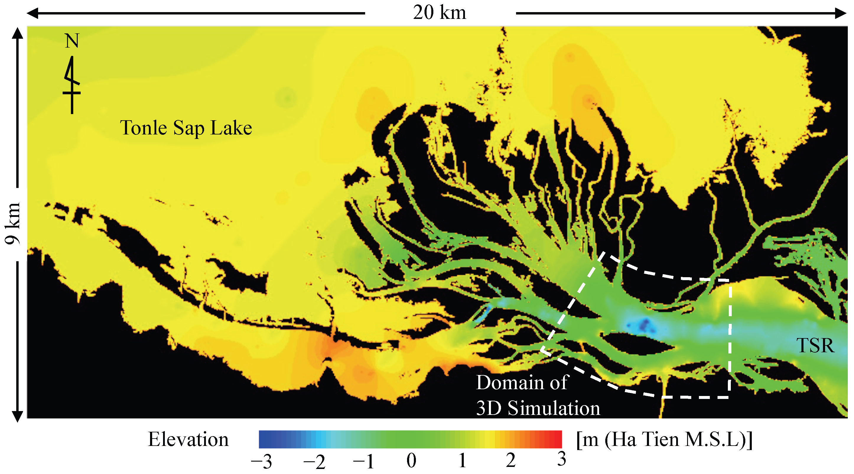
3.1. Topography of Water Channels

As illustrated in Figure 3, the Chhnok Tru floating village is located in the transitional area between the TSL and TSR. The village is located not in the main channel of the TSR but in the southern sub-channels branching off from the TSR. Furthermore, upstream between the village and TSL, the TSR splits into many small channels that create a complex dendritic network of waterways. Under these complex topographic conditions, the availability of accurate topographic data is crucial to achieve realistic flow simulations.

Although the Mekong River Commission (MRC) provides a bathymetric map of the entire stream of the MR, including the TSR and TSL [23], the bathymetric data on the map are presented mainly for cross-sections of the main channels at relatively coarse intervals (every 400 m in the longitudinal direction of the channel). The depth of small sub-channels where the Chhnok Tru village is located is not adequately displayed on the map. Furthermore, due to active sediment deposition expected in the area, the depth and location of channels may differ from the MRC bathymetry map, which was created based on a sounding survey and aerial photos from over 20 years ago. Thus, in this study, we started the hydraulic simulation by creating a fine topographic map of the water channels near the village. The map was created as a digital elevation model (DEM) using the following three processes: (1) detecting both the location and network of water channels using satellite image analysis, (2) conducting a sounding survey in the sub-channels near the village, and (3) interpolating the elevation on each DEM mesh using a smooth profile provided by the biharmonic equation. Because a main part of the village is located in a sub-channel with a width of 200 m (see Figure 3), we aimed to create a DEM with a mesh size of 10 m.

3.1.1. Detection of Location and Network of Water Channels

To generate a fine DEM, we used a satellite image provided by the Sentinel-2 Multispectral Instrument (MSI). Figure 4a displays the satellite image in true color, which we employed. The satellite image was recorded in the middle of the dry season (10 March 2018) when the water level decreased to a sufficiently low level to clearly distinguish channels from sandbanks. The Sentinel-2 MSI measures electromagnetic reflectance on the land surface, ranging from visible to infrared wavelengths. Because water absorbs near-infrared light to a larger extent than visible green light, the water content on the land surface can be detected by evaluating the difference in reflectance between visible green and near-infrared light. The normalized difference water index (NDWI) [24,25] is an index based on this concept that is sensitive to water content on the land surface:

$$\mathrm{NDWI}=\frac{X_{green}-X_{nir}}{X_{green}+X_{nir}},$$

(12)

where $X_{green}$ and $X_{nir}$ denote the reflectance of visible green light (band-3; wavelength $\mathit{\lambda }=559$ nm) and near-infrared light (band-8; $\mathit{\lambda }=833$ nm), respectively. The reflectance values $X_{green}$ and $X_{nir}$ are provided as a digitized map with a mesh size of 10 m. In this study, the digital numbers of band-3 and band-8 were directly used for $X_{green}$ and $X_{nir}$, respectively, without conversion to raw reflectance values.

Figure 5 presents a scatter plot of the reflectance values at locations that can be clearly distinguished as either land surface or water surface in the true color image (Figure 4a). In the plot, different values of NDWI are represented as straight lines with different slopes. The NDWI values range from –1 to 1, with a higher value indicating a larger presence of water on the land surface. Dry surfaces, such as forests and paddy fields, are associated with lower NDWI values. Based on the scatter plot, we set $\mathrm{NDWI}=-0.2$ as the threshold value. Meshes with NDWI values higher than this threshold were considered to represent the water surface of channels. Figure 4b presents the detected water channels. A dendritic network of many small channels upstream of the Chhnok Tru village is clearly detected.

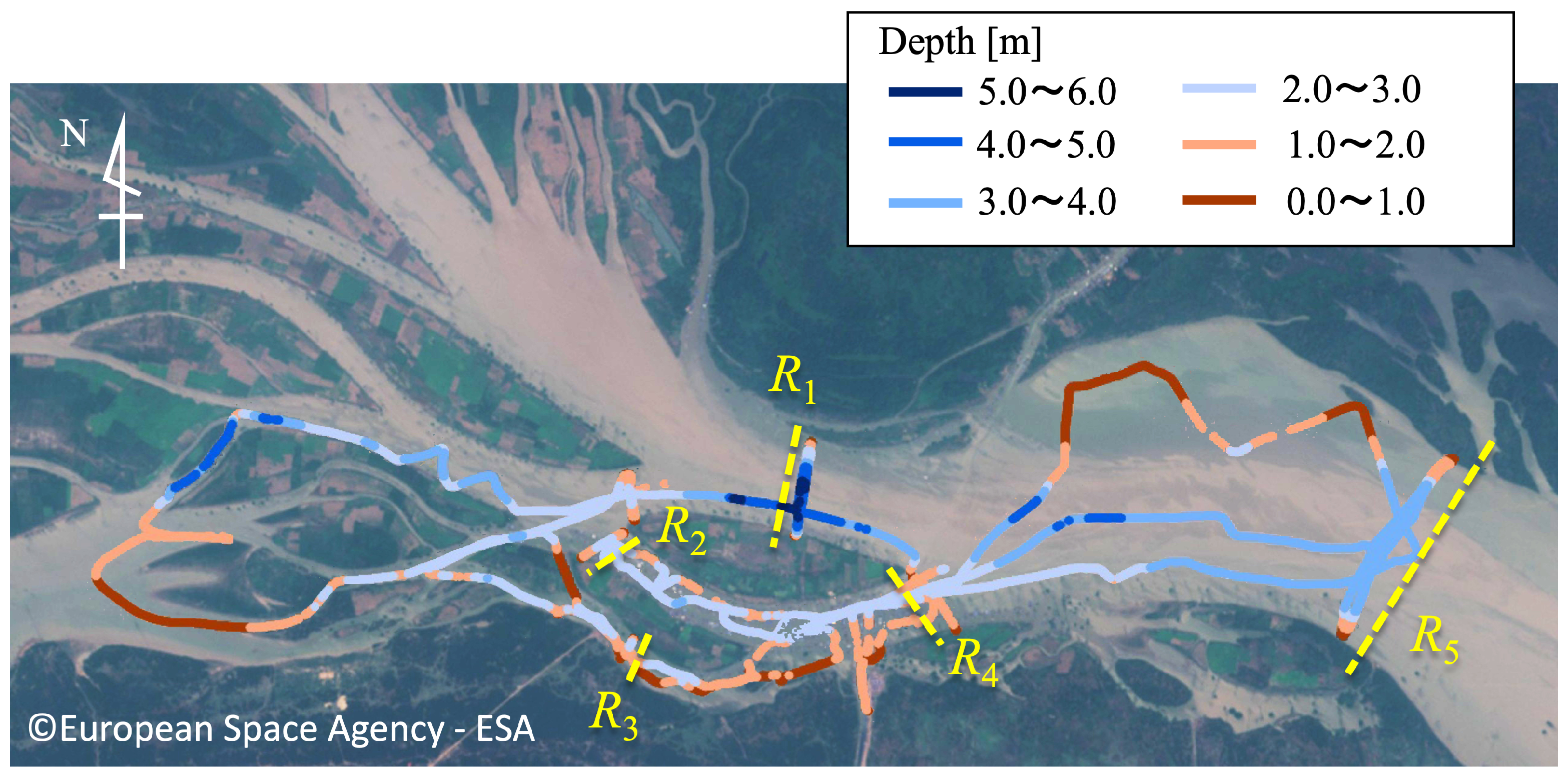
3.1.2. Sounding Survey

To compensate for the lack of bathymetric data for the small sub-channels where the Chhnok Tru village is located, we conducted a sounding survey on 7 March 2018, three days before the recording of the satellite image used for the NDWI analysis. An acoustic Doppler current profiler (ADCP) unit (River Surveyor M9, SonTek/Xylem) was employed. The ADCP had eight transducers for flow velocity profiling and one vertical transducer for water depth observation. To measure the flow velocity with a measurement error of 1% or 0.2 cm/s, the water depth was measured by irradiating a 0.5 MHz ultrasonic wave vertically downward and recording the reflections. In the survey, the ADCP was installed on the side of a small FRP boat. By driving the boat in a zigzag pattern (Figure 6), spatially dense data were captured across the entire area of the village. In the field observation, in addition to the sounding survey, the flow rate was measured at the five cross-sections indicated by yellow lines in Figure 6. The measured flow rate is presented in

Table 1. Flow rate at cross-sections $R_1$–$R_5$ in the Chhnok Tru floating village. Observational data obtained by ADCP and flow rates calculated by 2D and 3D hydraulic models are provided.

	${\mathit{R}}_1$ [m3/s]	${\mathit{R}}_2$ [m3/s]	${\mathit{R}}_3$ [m3/s]	${\mathit{R}}_4$ [m3/s]	${\mathit{R}}_5$ [m3/s]
Observation	480.3 ± 37.3	61.0 ± 0.6	37.4 ± 5.9	98.5 ± 6.6	586.5 ± 43.9
Simulation (2D model)	437.0	82.0	29.9	102.4	582.9
Simulation (3D model)	421.0	98.3	29.2	124.5	- †

Note: ^† $R_5$ cross-section located outside of computational domain.

.

3.1.3. Interpolation Using a Biharmonic Equation

A DEM was created by spatially interpolating the observational results of the sounding survey and the bathymetric data provided by MRC’s map. A rectangular area encompassing the village, measuring 20 km from east to west and 9 km from north to south, was digitized using a uniform Cartesian mesh with a width of 10 m (see Figure 7). To interpolate the bed surface of the channels with a smooth profile, we employed the following biharmonic equation:

$$\frac{{\mathsf{\partial }}^{4}Z}{\mathsf{\partial }{x}^4}+\frac{{\mathsf{\partial }}^{4}Z}{\mathsf{\partial }{x}^2\mathsf{\partial }{y}^2}+\frac{{\mathsf{\partial }}^{4}Z}{\mathsf{\partial }{y}^4}=\sum _m{Z}_m^{obs}\mathit{\delta }\left(x-x_m^{obs},y-y_m^{obs}\right),$$

(13)

where $Z(x,y)$ represents the interpolated elevation of the bed surface of the water channels. $x_m^{obs},y_m^{obs}$ are the horizontal coordinates, and the elevation $Z_m^{obs}$ is provided by the sounding survey and MRC’s bathymetric map. The smoothness of the spatial profile is indicated by the total square of curvature:

$$T=\int \int {\left(\frac{{\mathsf{\partial }}^{2}Z}{\mathsf{\partial }{x}^2}+\frac{{\mathsf{\partial }}^{2}Z}{\mathsf{\partial }{y}^2}\right)}^{2}dxdy$$

(14)

Smaller values of T imply a smoother profile of Z. Briggs demonstrated that the solution of the biharmonic Equation (13) minimizes T [26]. In this study, the biharmonic Equation (13) was discretized on the DEM mesh by applying the finite difference method and solved using the BiCGstab method. After interpolating the elevation of the bottom surface of the water channels, the elevation of DEM meshes, which were located on land, was patched using the DEM of the NASA Shuttle Radar Topography Mission 3 arc-second global (SRTM3) [27]. Figure 8 displays the resulting DEM.

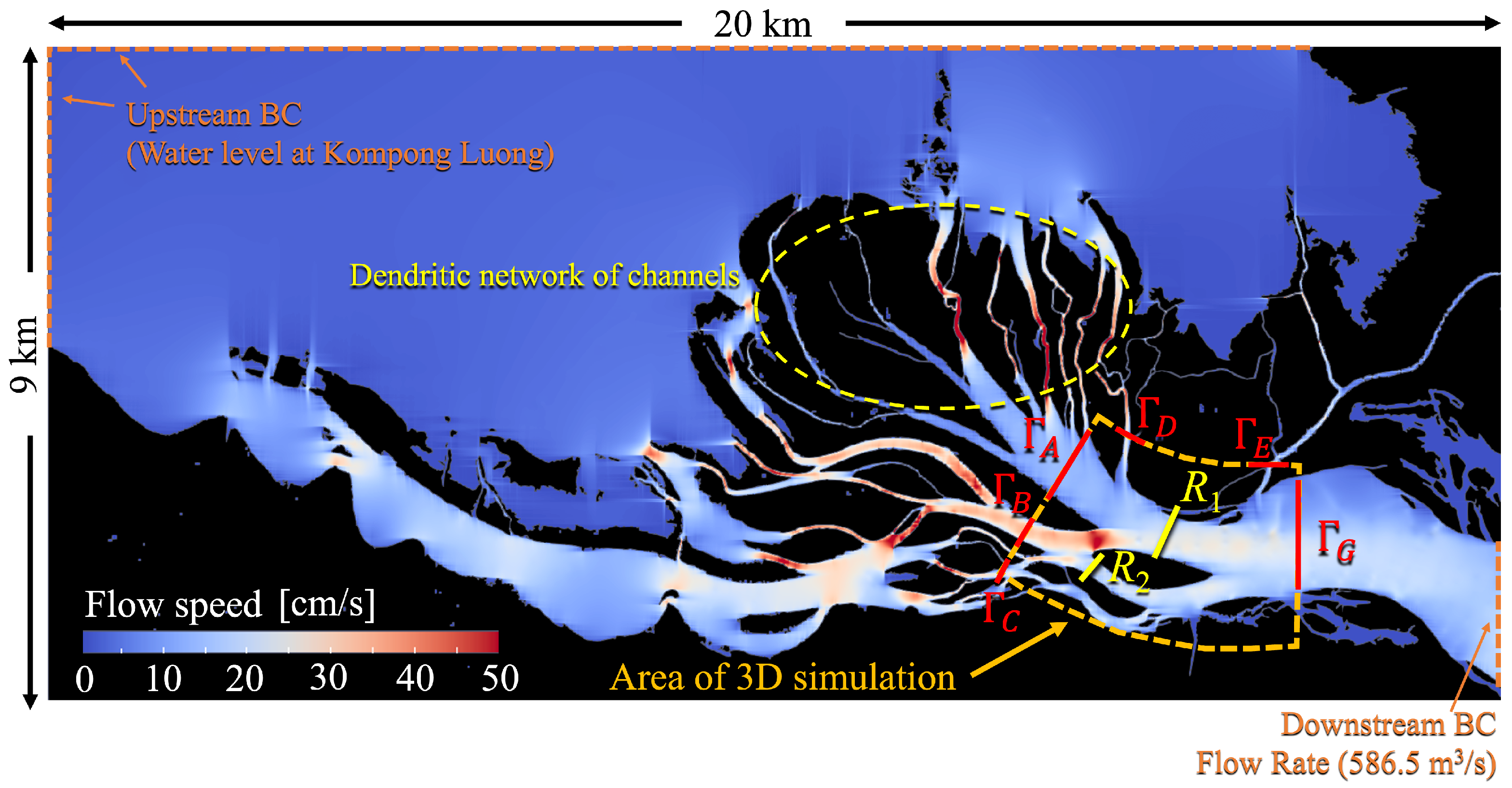
3.2. Flow Rate of Water Channels

Small channels form the complex dendritic network upstream of the Chhnok Tru village. Water flows from the TSL into the village through the various routes of the network. To simulate the flow in the village, the flow rates of individual small upstream channels were necessary as the boundary condition. However, because information regarding the flow rate was not available, we employed a 2D hydraulic model to estimate the flow rate. The computational domain was set to the entire area of the DEM displayed in Figure 7. Although the domain was wide (20 km × 9 km), encompassing both the village and upstream channel network, a fine mesh size of 10 m was used to represent narrow channels. To address the long computational time caused by the fine mesh, we applied a newly developed 2D model. This model solves the shallow water equation and accelerates the simulation to be 100 times faster than a conventional model through massive parallel computation using the general-purpose computing on graphics processing units (GPGPU) method (see [28] for details). The model has already been applied to the flow simulation in the same water area as this study, while the area is expanded to include the whole TSL and TSR [28]. In that previous work, it had been confirmed that the model has enough performance to effectively restore the seasonal rising/descending of water level in the TSL with accuracy, and the Manning’s roughness coefficient had been optimized, being based on the observational data. We employed the same Manning’s coefficient of $n=0.035$ in the present work.

The simulation was performed for the day of the sounding survey conducted using the ADCP (7 March 2018). The observed water level at the Kompong Luong gauge station in the TSL was used as the upstream boundary condition, while the observed flow rate was imposed at the downstream boundary in the TSR. Figure 9 presents the depth-averaged flow velocity calculated after a 3-day run-up calculation. A comparison with the observational flow rate is presented in Table 1. The flow rates of the 2D model at cross-sections $R_1-R_5$ were calculated by integrating the flow velocity along the cross-sections. The total amount of water flowing from the TSL to the TSR (flow rate at cross-section $R_5$) is in good agreement with the observational data. While the model overestimated at the southern cross-section $R_2$, the flow rate at the northern cross-section $R_1$ was underestimated. As one of the causes of this difference between the observation and simulation, we suspect that the water channels between the TSL and $R_1$ were simulated with slower flow than in actual fact. As shown in Figure 9, the southern channel where $R_2$ is located connects to relatively wide channels in the upstream between ${\Gamma }_B$ and the TSL. On the other hand, the northern channel where $R_1$ is located connects into a dendritic network consisting of many narrow channels between ${\Gamma }_A$ and the TSL (the yellow dashed circle shown in Figure 9). Although the DEM was generated with the relatively fine mesh size of 10 m, there are possibly channels ignored in the DEM due to having a width narrower than the mesh size. Furthermore, a limitation of the satellite imagery analysis makes the proper detection of the narrow channel more difficult. As shown in Figure 10, in the dendritic network in the upstream of $R_1$, the water surface could be covered by flooded forests and clusters of floating water hyacinth. When the authors visited the site and conducted the sounding survey with a small boat, we observed upstream of the floating village that the whole water surface of the many narrow channels was completely covered with the water hyacinth, making it impossible for the boat to proceed. Because the water surface covered by the vegetation cannot be detected by the satellite imagery analysis with the NDWI, some channels upstream of $R_1$ may have been ignored or misidentified as narrower. We think that these DEMs are an insufficient representation of the narrow channels, as they caused the inflow from the TSL to $R_1$ to decrease and the inflow to $R_2$ to increase, as compensation.

4. 3D Hydraulic Simulation for Chhnok Tru Village

Using the generated topographic data and estimated flow rates, we performed 3D hydraulic simulation to determine the flow regime and transport of E. coli using TITech-WARM. While the hydraulic conditions of the TSL change drastically between the dry season (November to April) and wet season (May to October), water pollution due to floating houses in the dry season is expected to be more severe than that in the wet season. This is because there is weakening of the concentration of contaminants, due to both dilution of pollution and transport of contaminated water away from the village, in the wet season, when the water current and water level increase. Based on this consideration, we focused on the dry season in this work. Specifically, we selected the day of the sounding survey (7 March 2018) as the target due to data availability and performed a hydraulic simulation of both water flow and pathogen transport.

4.1. Computational Conditions of Water Flow

The computational domain was set to a 3.6 km section in the longitudinal direction of the TSR (Figure 8). The domain contained both the main channel and sub-channels in which the village was located. The horizontal mesh size was set to 20 m in both the longitudinal and transverse directions of the channel. In the vertical direction, 20 computational grid points were used, independent of water depth. The simulation was performed for one day (7 March 2018). After a run-up calculation was performed for 6 days under the same conditions, the spatiotemporal changes in water flow over 24 h were simulated.

As shown in Figure 8, a total of seven boundaries ${\Gamma }_A$–${\Gamma }_G$ are set in the 3D simulation. Here, we would like to note that locations of the boundaries ${\Gamma }_A$–${\Gamma }_G$ are different from the cross-sections $R_1$–$R_5$, where the flow rate was measured by the ADCP. Among the seven boundaries, for the five boundaries ${\Gamma }_A$–${\Gamma }_E$, the flow rates calculated by the 2D hydraulic model were used as boundary conditions. The location of the ${\Gamma }_A$–${\Gamma }_E$ in the computational domain of the 2D simulation is shown in Figure 9. Firstly, the flow rate at each boundary ${\Gamma }_A$–${\Gamma }_E$ was calculated by integrating the depth-averaged flow velocity calculated with the 2D model. Then, the calculated flow rate was inputted to the 3D model and the velocity on ${\Gamma }_A$–${\Gamma }_E$ was set. The 2D model calculates the transverse profile of the depth-averaged flow velocity and ideally we can utilize that information to set a spatial transverse profile of the velocity on each boundary ${\Gamma }_A$–${\Gamma }_E$ in the 3D model. However, due to a technical limitation of the TITech-WARM, which is the 3D model used in this work, the velocity was assumed to be uniform in each cross-section and was set to a constant value, estimated by dividing the inputted flow rate by the surface of each cross-section. Boundary ${\Gamma }_F$ was located at the entrance of a short canal ending approximately 500 m away. Because the canal lacked any inflow, we set the wall boundary condition to ${\Gamma }_F$. At the downstream boundary ${\Gamma }_G$, the Neumann condition was applied to both velocity and temperature, and the water level was set to the cross-sectional average of the calculated results of the 2D simulation. The boundary conditions are summarized in

Table 2. Boundary conditions for 3D hydraulic simulation.

${\Gamma }_A$	Inflow boundary	${\Gamma }_E$	Inflow boundary
	Constant flow rate ($Q=176.9$ m/s) *		Constant flow rate ($Q=23.6$ m/s) *
	Observed water temperature **		Observed water temperature **
${\Gamma }_B$	Inflow boundary	${\Gamma }_F$	Wall boundary
	Constant flow rate ($Q=260.8$ m/s) *		Zero flow rate $Q=0$ m/s
	Observed water temperature **
${\Gamma }_C$	Inflow boundary	${\Gamma }_G$	Outflow boundary
	Constant flow rate ($Q=78.1$ m/s) *		$\mathsf{\partial }\mathbf{u}/\mathsf{\partial }x=\mathsf{\partial }T/\mathsf{\partial }x=0$
	Observed water temperature **		Constant water level ($h=2.295$ m) *
${\Gamma }_D$	Inflow boundary
	Constant flow rate ($Q=32.5$ m/s) *
	Observed water temperature **

Note: * Flow rate Q and water level h calculated by 2D simulation. ** Hourly data observed on water surface in the upstream.

.

The initial conditions were set as follows. The velocity was set to zero for the entire area, the water level was set to the average of the calculated results of the 2D hydraulic simulation, and the water temperature was set to the uniform temperature measured at the center of the village on the target day. To evaluate the wind frictional force and heat exchange on the water surface, we input hourly meteorological data, which were prepared by averaging data observed in March 2019. Obstruction of water flow by the floating houses was not modeled in the simulation.

4.2. Computational Conditions of E. coli Transport

The input of E. coli from each house to the water was modeled as follows. First, the location of each house in the village was determined using satellite imagery. Because the spatial resolution of Sentinel-2 satellite images was insufficient to clearly distinguish each house on the target day, we used images provided by Google Earth. The images were taken on 1 January 2017, approximately two months before the target day (7 March 2018). Both January and March fall within the dry season and have low water levels. Furthermore, it was reported by many residents that relocation of houses to other villages is infrequent. Therefore, we assumed that the discrepancy in the image recording day had a negligible impact on the location of houses or the population of the village. Based on the satellite images, we determined the locations of 1362 houses.

The next step was to determine the amount of E. coli excreted from each house. We assumed five family members in each house, which is the average household size in Cambodia [29]. The amount of feces excreted is dependent on what individuals consume. Tanaka et al. measured the weight of fresh feces of Japanese individuals following a rice-containing diet [30]. Because rice is a staple food in Cambodia as well as Japan, we assumed that each resident in the village excreted 105 g of feces per day, which is the average for males, as reported by Tanaka et al. Furthermore, referring to a study by Ervin et al. [31], we assumed that an E. coli amount of ${10}^9$ CFU was contained per gram of feces. Combining the above assumptions, the total amount of E. coli excreted from one house in one day was calculated as $5\times 105\times {10}^9=5.25\times {10}^{11}$ CFU per house.

We assumed that all houses excreted E. coli every morning and that the time of excretion was distributed randomly during a 4 h period around sunrise (from 4:00 to 8:00). This timeframe was based on reports from the residents about their daily routine. In the calculation, the concentration of E. coli in the computational mesh of the water surface where each house was located was increased at the excretion time, assuming that the excreted E. coli was momentarily diluted in the mesh.

Because of a lack of information regarding the pollution of bottom sediments with E. coli in the target site, absorption and elution of E. coli to/from the bottom sediments were not modeled in this work. Some recent research reports that E. coli are detected at high concentrations in the bottom sediments of the rivers [32,33]. Furthermore, some experimental studies, which measured temporal reduction in E. coli in the river bottom mud incubated at a certain temperature, report that E. coli can survive in the sediments for more than a month [34,35]. This research related to the bottom sediments suggests that the sediments may have an influence on E. coli concentration and distribution in water; the modeling of the influence of the bottom sediments is expected to enable a more reliable analysis of E. coli transport.

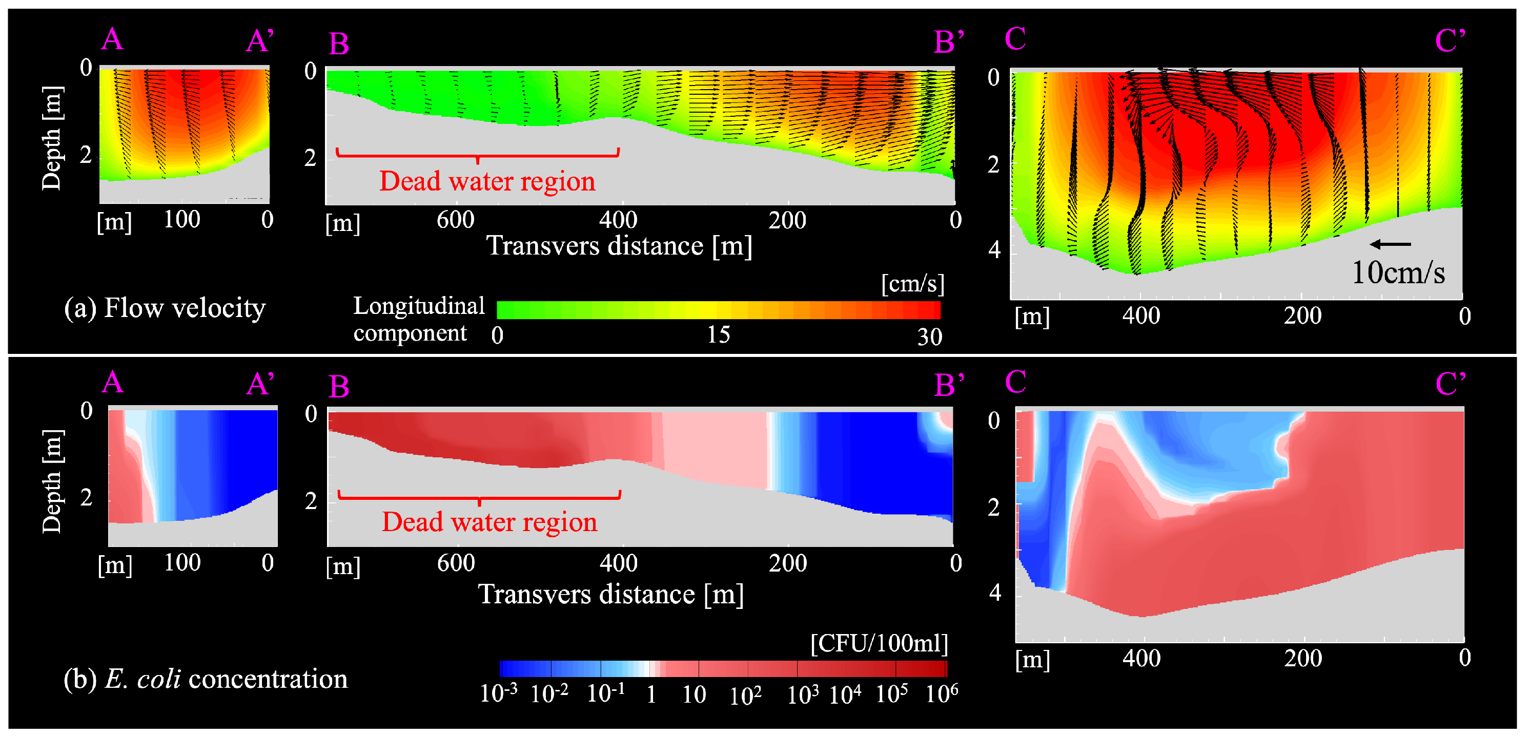
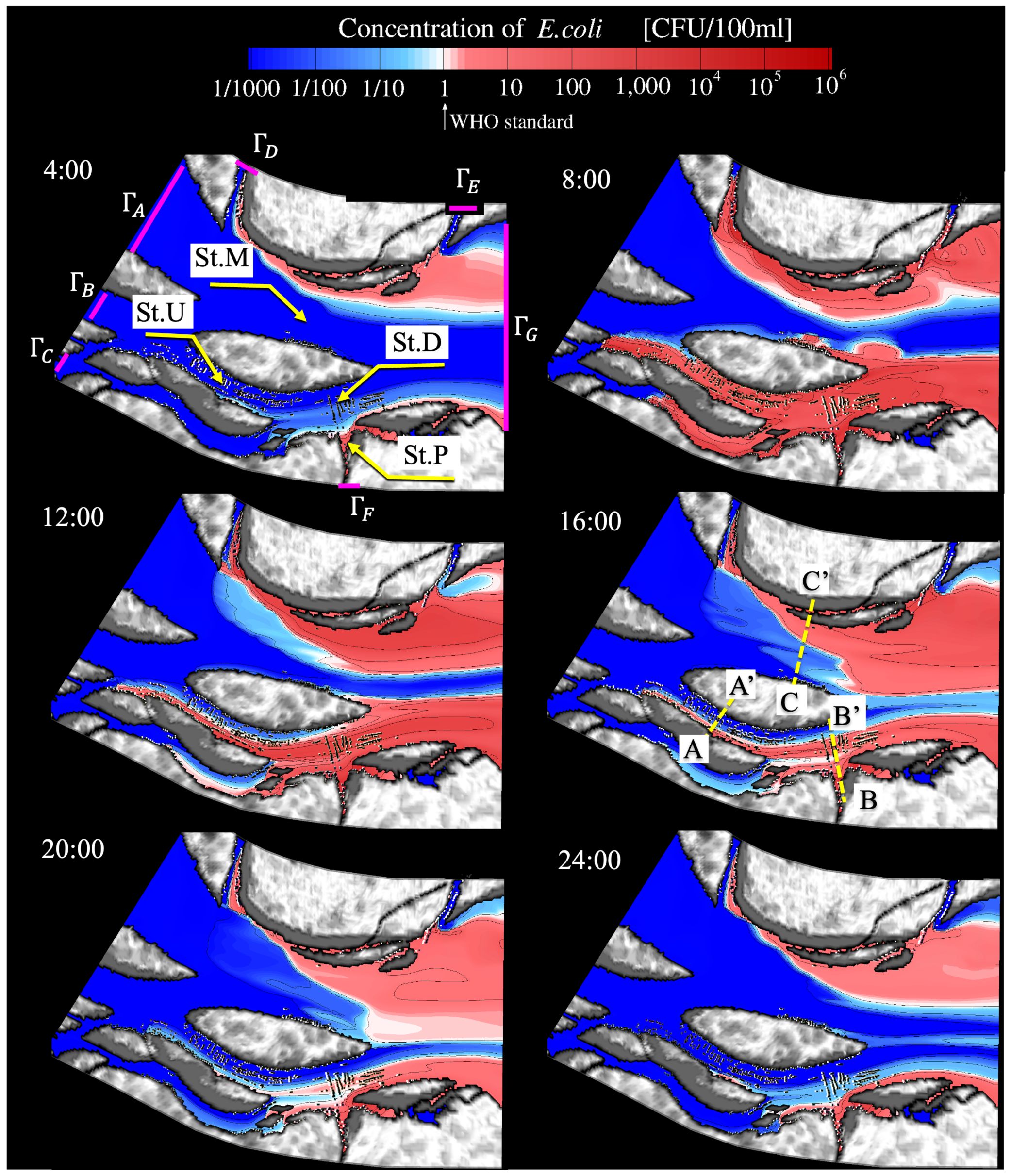
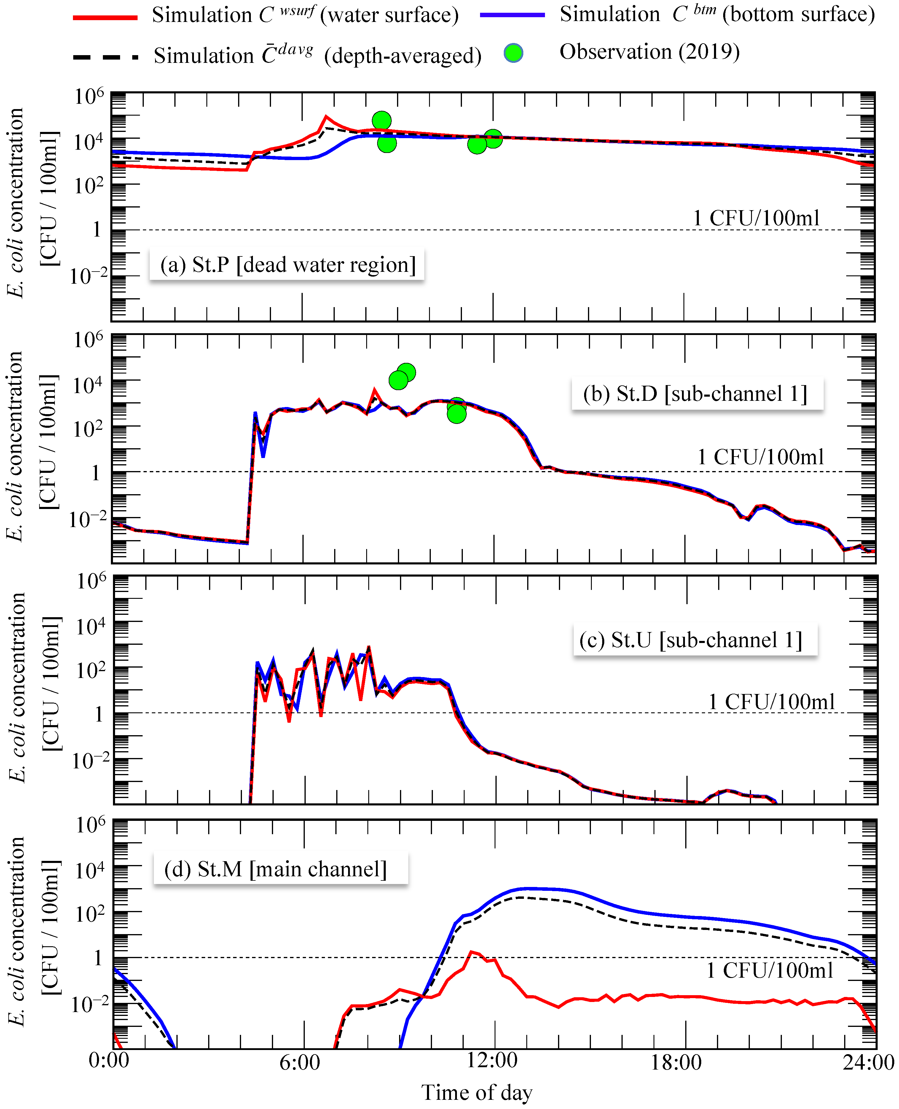
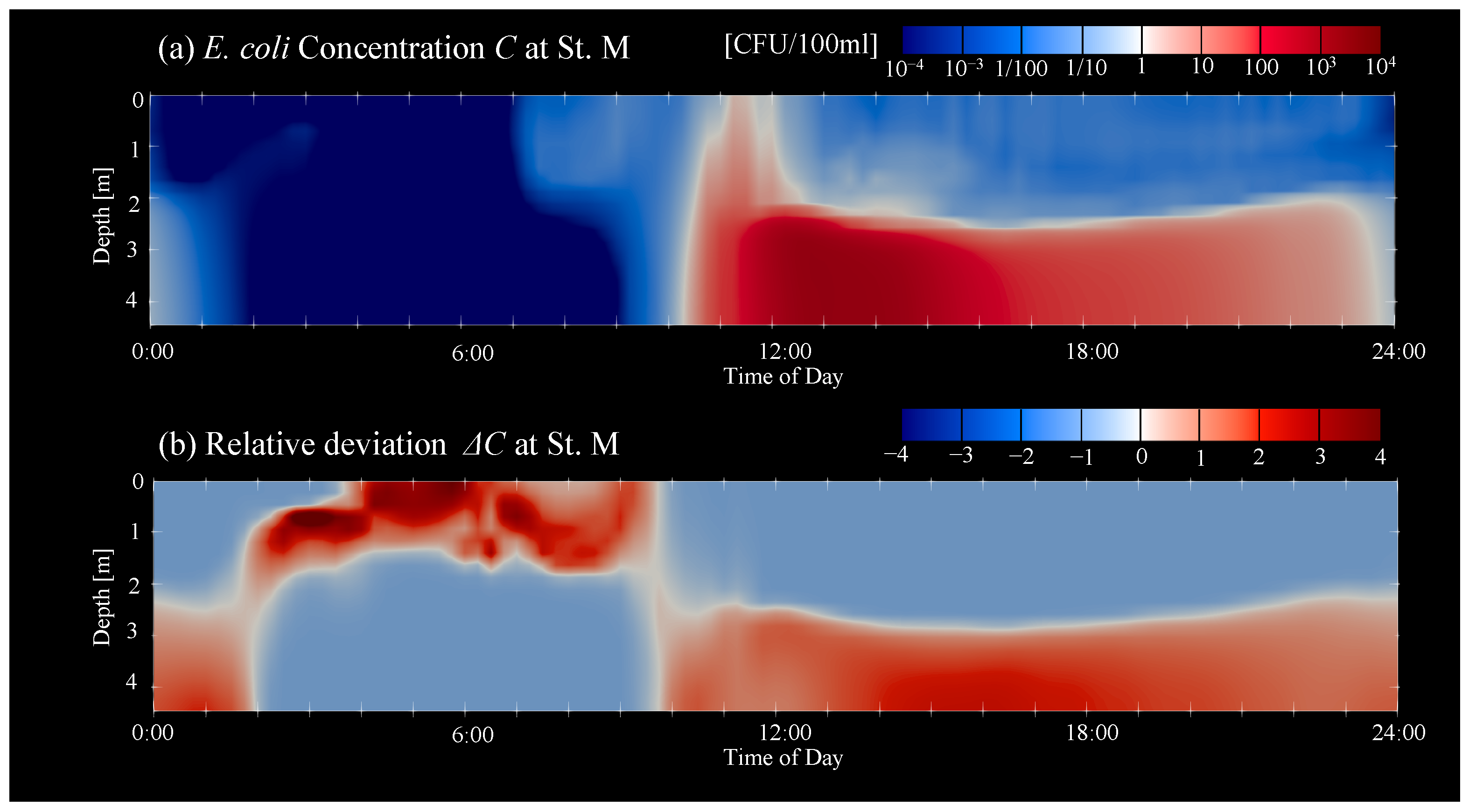
4.3. Calculation Results

Figure 11 presents the calculation results of the longitudinal flow velocity at the water surface. Black dots represent the locations of floating houses. From this result, we observed the following characteristics of the flow regime in the village. First, a rapid flow flows into the village from the relatively narrow channel ${\Gamma }_B$ rather than the wide channel ${\Gamma }_A$. In addition, the largest flow from ${\Gamma }_B$ is divided into the main channel on the north side and sub-channel 1 on the south side at branch $P_F$ (see Figure 3 for the location of the mentioned channels). While the flow speed in southern sub-channel 1, which is in the central area of the village where many floating houses are located, is relatively fast (20 cm/s∼30 cm/s), in the dented area around ${\Gamma }_F$, which is the entrance of a short canal clogged 500 m away, the water flow is stagnated with a slow speed, and the area appears to be a dead water region. Figure 12a presents the velocity profile at several cross-sections. The location of each cross-section is indicated by a violet dashed line in Figure 11. In Figure 12, longitudinal and other components are indicated by color contours and arrows, respectively. From cross-section B-B${}^{\prime }$, it is confirmed that a dead water region is generated around the mouth of the canal. Furthermore, the flow speed near the bottom is attenuated due to friction in all cross-sections. In cross-section C-C${}^{\prime }$, circular flow is clearly observed, which is probably secondary flow due to the bending of the channel.

Table 1 presents the flow rates estimated by integrating the calculated velocity at cross-sections $R_1$–$R_4$, displayed in Figure 6. In the table, the flow rate in the morning (8:00), when feces were excreted from houses, is provided as the simulation result of the 3D model. As well as the flow rate calculated by the 2D model, the flow rate at cross-section $R_1$ is smaller than the observation, while the flow rate $R_2$ is larger than the measurement. This difference is expected to be caused by the insufficient representation of the narrow channels in the upstream, as discussed in the preparation of flow rate with the prior 2D simulation (see Section 3.2). Other than this difference, with a similar tendency as the 2D model, the flow rate of the 3D model differs from the 2D model, as shown most clearly at cross-section $R_4$. In the 3D simulation, a bottom-frictional coefficient was set to be the same value as the Manning’s roughness coefficient optimized for the 2D simulation. However, because the bottom-frictional force in the 3D simulation is modeled not with the depth-averaged velocity but with the local speed at the bottom surface, the non-proper frictional force probably was evaluated in the 3D simulation differently from the 2D simulation. We think that this is a cause for the difference in the flow rate between the 3D and 2D models. By adjusting the bottom-frictional coefficient, the flow rate is expected to be close to the 2D simulation.

Figure 13 displays the calculated daily change in the concentration of E. coli at the water surface. In the guidelines for drinking water published by the World Health Organization (WHO) [36], it is specified that E. coli should not be detected in a 100 ml water sample. In Figure 13, to illustrate the spatial distribution of contaminated water, an E. coli concentration exceeding the WHO standard ($C>1$ CFU/100 mL ) is colored in red. The results indicate that the reduction rate of E. coli concentration strongly depends on location due to spatial changes in water flow. As illustrated in Figure 13, in a channel (sub-channel 1 in Figure 3) at the center of the village where many houses are located (denoted St. U in Figure 13), the concentration decreases to meet the WHO standard ($C<1$ CFU /100 mL) in early afternoon due to relatively rapid water flow. In contrast, in stagnant water areas such as a clogged canal (St. P in Figure 13), the concentration remains 1000 times higher than the WHO standard throughout the day. This variation in reduction rates suggests that the disease risk of pathogenic E. coli can be reduced by selecting appropriate times and locations to withdraw lake water for drinking (e.g., in the evening upstream of a central area where houses are not crowded and the water flow is relatively rapid).

Figure 14 illustrates the temporal changes in E. coli concentration at the various locations. While red and blue curves represent the concentration at the water surface $C^{wsurf}=C\left(t,x,y,z=h\right)$ and bottom surface $C^{btm}=C\left(t,x,y,z=b\right)$, respectively, the black dashed curve shows the depth-averaged concentration that was calculated by

$${\overline{C}}^{davg}=\frac{1}{h-b}{\int }_b^{h}C\left(t,x,y,z\right)dz.$$

(15)

In addition to the calculated E. coli concentration, the observational data are indicated by green circles. The field measurement of E. coli was performed at the water surface around St. P and St. D on 14–15 March 2019, almost one year after the simulation period. Although the verification is not entirely accurate because the year differs from the simulation year, the observed data are in good agreement with the calculation results, and the simulation appears to calculate reasonable E. coli transport.

Figure 12b displays the vertical transverse profile of the E. coli concentration at the cross-sections. Whereas the E. coli concentration is almost uniform in the vertical direction in shallow and narrow sub-channels, in cross-section C-C${}^{\prime }$ of the wide main channel, dangerous levels of E. coli are transported from side C${}^{\prime }$ to side C along the bottom bed, creating a tongue shape. This transverse transport signifies that pathogens from the northern area (see Figure 3) can move and affect residents living on the opposite southern shore without their awareness. As evident by comparing the cross-section of the velocity displayed in Figure 12a, the existence of secondary flow is responsible for this silent invasion of pathogens beneath the water surface.

Here, we would like to illustrate the difference between the 3D model and 2D model. In comparison with the depth-averaged 2D model, although the 3D model needs a larger computational effort and takes more time, the 3D model has the advantage that the vertical profile can be grasped. In each panel of Figure 14, the diurnal change in $C^{wsurf}$, $C^{btm}$, and ${\overline{C}}^{davg}$ is shown by a red solid curve, a blue solid curve, and a black dashed curve, respectively. Because the depth-averaged concentration ${\overline{C}}^{davg}$ is the target variable that we could determine by applying the 2D hydraulic model, the deviation of $C^{wsurf}$ and $C^{btm}$ from ${\overline{C}}^{davg}$ suggests to us the expected difference between the 3D and 2D solutions. As shown in Figure 14b,c, at St. D and St. U, which are in the center of the shallow sub-channel 1, both $C^{wsurf}$ and $C^{btm}$ almost agree with ${\overline{C}}^{davg}$. Generally speaking, it can be expected that the vertical profile of water flow and substances may be uniform in shallow water areas. Actually, it was found in the calculated results that the E. coli concentration tends to be uniform over a wide area, not just at St. D and St. U. However, in some areas where the flow velocity changes in a vertical direction due to topographic conditions, there was a large vertical deviation in the E. coli concentration that could not be ignored. As shown in Figure 14d, at St. M, both $C^{btm}$ and ${\overline{C}}^{davg}$ drastically increase before noon and remain about 1000 times higher than $C^{wsurf}$ throughout the afternoon. Figure 15 shows the temporal change in the vertical profile of E. coli concentration at St. M. In addition to the raw concentration C, a vertical profile of relative deviation $\Delta C$, which indicates the difference from the depth-averaged concentration ${\overline{C}}^{davg}$, is also shown in panel (b):

$$\Delta C=\left(C-{\overline{C}}^{davg}\right)/{\overline{C}}^{davg}.$$

(16)

It can be seen that a thick water layer of high concentration exists throughout the afternoon at depths deeper than 2 m. Because St. M is located on cross-section C-C${}^{\prime }$ in the main channel (see Figure 13), the long-term existence of the thick high-concentration bottom layer can be interpreted to mean that the transverse transport of E. coli along the bottom of cross-section C-C${}^{\prime }$, which is discussed in the above regarding Figure 12b, continues throughout the afternoon. As shown in Figure 15b, the relative deviation at the water surface is kept at $\Delta C\approx -1$ in the afternoon. It means that $C^{wsurf}$ is almost 100% less than ${\overline{C}}^{davg}$ and the 2D model would possibly overestimate the concentration in comparison with the 3D model. Furthermore, as shown in Figure 14a, at St. P, which is in the dead water area where the water flow is stagnated, we can see a clear difference among $C^{wsurf}$, $C^{btm}$, and ${\overline{C}}^{davg}$ both at night (from 0:00 to 4:00) and in the morning (from 4:00 to 12:00). Figure 16 shows the vertical profile of C and $\Delta C$ at St. P. At night before 4:00 when the E. coli is not excreted from the floating houses, E. coli concentration remains relatively higher in the deeper area along the bottom. This is thought to be because there is no strong flow in the dead water region and even the remaining weak flow is further slowed near the bottom due to frictional force (see the panel of cross-section B-B${}^{\prime }$ in Figure 12b), so exchange of the polluted water with the outside unpolluted water becomes selectively weak in the bottom layer. Conversely, in the morning from 4:00 to noon, the concentration in the upper layer is larger than in the bottom layer because the E. coli is excreted from the houses on the water surface between 4:00 and 8:00. As shown in Figure 16b, the relative deviation $\Delta C$ at the water surface fluctuates largely during the above-mentioned two periods. At the water surface, while $\Delta C$ is approximately −0.5 at night between 0:00 and 4:00, $\Delta C$ remains larger than 1 and reaches up to $\Delta C\approx 2$ at most in the morning between 4:00 and 12:00. In the present work, as described in the later chapter, ingestion of the pathogen into the body was evaluated from the daily averaged E. coli concentration in the water and the disease probability is assessed by the amount of the ingestion. Because residents scoop drinking water from the water surface by ladles and swim near the water surface, the E. coli concentration at the water surface $C^{wsurf}$ was used for the evaluation of the ingestion.

Table 3. Daily averaged E. coli concentration ${\overline{C}}_{day}$ and disease probability over 3 months $P_{93}$ at St. M and St. P. Superscripts $wsurf$ and $davg$ represent the values evaluated with the concentration at the water surface $C^{wsurf}$ and depth-averaged concentration $C^{davg}$, respectively.

	Daily Averaged E. coli Concentration †			Disease Probability over 3 Months ‡
	${\overline{\mathit{C}}}_{\mathit{day}}^{\mathit{wsurf}}$	${\overline{\mathit{C}}}_{\mathit{day}}^{\mathit{davg}}$	${\overline{\mathit{C}}}_{\mathit{day}}^{\mathit{davg}}-{\overline{\mathit{C}}}_{\mathit{day}}^{\mathit{wsurf}}$	${\mathit{P}}_{\mathit{93}}^{\mathit{wsurf}}$	${\mathit{P}}_{\mathit{93}}^{\mathit{davg}}$	${\mathit{P}}_{\mathit{93}}^{\mathit{davg}}-{\mathit{P}}_{\mathit{93}}^{\mathit{wsurf}}$
St. M	0.07	49.57	49.50	0.00021	0.012	0.01179
St. P	8441	6962	−1479	0.86	0.80	−0.06

Note: ^† Unit is CFU/100 mL. ^‡ Probability that one resident contracts a disease at least once over 93 days.

shows the results of a trial calculation of the daily averaged concentration ${\overline{C}}_{day}$ and the disease probability over 3 months $P_{93}$ when using the water surface concentration $C^{wsurf}$ and the depth-averaged concentration ${\overline{C}}^{davg}$, respectively, for St. P and St. M, where a clear difference was observed between $C^{wsurf}$ and ${\overline{C}}^{davg}$. At St. P, the depth-averaged concentration (${\overline{C}}_{day}^{davg}$ = 6962 CFU/100 mL) is about 20% smaller than the concentration at the water surface (${\overline{C}}_{day}^{wsurf}$ = 8441 CFU/100 mL). As a result, in comparison with the probability ($P_{93}^{wsurf}$ = 0.86) using the concentration at the water surface, the disease probability ($P_{93}^{davg}$ = 0.80) with the depth-averaged concentration is underestimated by 0.06. As suggested from the fact that this underestimation is equivalent to 7.5% of the $P_{93}^{wsurf}$, the difference between $C^{wsurf}$ and ${\overline{C}}^{davg}$, namely between the 3D simulation and the depth-averaged 2D simulation, possibly causes a non-negligible influence on disease risk assessment in some cases.

As demonstrated by this simulation, the simulation of E. coli by a hydraulic model can provide compelling evidence to support environmental awareness and encourage residents to change their behavior to access safe water. Furthermore, it should be noted that these 3D flow profiles indicating vertical changes in flow cannot be calculated using a 2D hydraulic model. Sometimes, 3D flow profiles are crucial for assessing pathogen contamination in water and evaluating the risk of waterborne diseases. This is because people can become infected with pathogens by consuming lake water from the water surface. Therefore, the transport of pathogens at the water surface should not be considered using the depth-averaged flow but using the flow at the water surface. Furthermore, to model phenomena selectively occurring at a certain depth such as the absorption to/elution from the bottom sediments and pasteurization by solar irradiation at the water surface, a local concentration at a certain depth instead of the depth-averaged concentration, namely the vertical profile of the concentration, must be simulated with a 3D model. The applications to these phenomena would highlight the further potential advantages of a 3D model.

5. Hazard Map Creation with QMRA

To create a useful risk map for the residents, concrete information about the probability of diseases should be illustrated. Furthermore, information about the number of expected diseases can help policy-makers compare the effectiveness of countermeasures and select which measures to introduce. In this section, we describe the application of QMRA to the simulated E. coli concentration and creation of the disease risk map.

5.1. Dose–Response Model

As the target diseases, we considered waterborne diseases caused by pathogenic E. coli, such as diarrhea, fever, and gastroenteritis. The probability of a resident contracting a disease during a certain period was evaluated using the following dose–response model of the beta-Poisson type [37]:

$$P_1\left(D\right)=1-{\left(1+\frac{D}{N_{50}}\left(2^{\frac{1}{\mathit{\alpha }}}-1\right)\right)}^{-\mathit{\alpha }},$$

(17)

where $P_1\left(D\right)$ denotes the probability of contracting a disease after ingesting D cells of pathogenic E. coli in a day. $\mathit{\alpha }$ and $N_{50}$ are model parameters set to $\mathit{\alpha }=0.1778$ and $N_{50}=8.6\times {10}^7$ based on the risk assessment conducted by Thi et al. for flooding in Hue city, Vietnam [37]. Various strains of E. coli are excreted from the human body. In the above 3D transport simulation, E. coli concentration C was modeled as the total of non-pathogenic and pathogenic strains. In contrast, Equation (17) is designed to evaluate disease risk from the number of ingested cells of pathogenic strains. Therefore, the risk evaluated by Equation (17) using the simulated E. coli concentration is expected to be overestimated. However, we did not apply any correction to interpret the simulated C as the pathogenic concentration. This was because we aimed to illustrate the relatively dangerous areas and the variation in disease risk within the village. We can convert $P_1\left(D\right)$ to the probability $P_d$ that people contract diseases over d days:

$$P_d=1-{\left(1-P\left(D\right)\right)}^d$$

(18)

5.2. Modeling of Ingestion

In this study, we assumed three processes for the ingestion of E. coli:

$$D=D_{drink}+D_{accident}+D_{vegetable}[\mathrm{CFU}/\mathrm{day}],$$

(19)

where $D_{drink}$, $D_{accident}$, and $D_{vegetable}$ represent ingestion by drinking lake water, accidental ingestion, and ingestion by eating contaminated vegetables, respectively. Although some residents in the floating village purchase treated bottled water that is safe to drink, a recent questionnaire survey revealed that approximately half of the residents have used lake water for drinking purposes and that approximately 30% of the lake water was raw and untreated [10]. To assess the disease risk due to drinking such untreated water, we modeled the drinking of raw lake water as one of the ingestion processes, and $D_{drink}$ was evaluated from the E. coli concentration calculated by the 3D simulation:

$$D_{drink}=L_{drink}\times {\overline{C}}_{day}^{wsurf},$$

(20)

where $L_{drink}$ represents the volume of water that an adult drinks per day. We assumed $L_{drink}=2.6$ L/day, which is the median water intake for adults [38]. Although the E. coli concentration C changes greatly over time even in the same location, we used the daily average E. coli concentration at the water surface ${\overline{C}}_{day}^{wsurf}$ due to the lack of detailed information on when residents withdrew lake water.

Many residents in the floating village work for fisheries. They often swim in the lake to set up fishing nets and harvest fish. In addition, residents commonly take baths in the lake water. Accidental drinking of lake water during fishing and bathing was considered the second ingestion process, $D_{accident}$:

$$D_{accident}=L_{fishing}\times {\overline{C}}_{day}^{wsurf}+L_{bathing}\times {\overline{C}}_{day}^{wsurf}$$

(21)

$L_{fishing}$ and $L_{bathing}$ were evaluated from the active time and ingestion ratio for each activity:

$$\begin{array}{ccc}& & L_{fishing}=T_{fishing}\times R_{fishing},\hfill \end{array}$$

(22)

$$\begin{array}{ccc}& & L_{bathing}=T_{bathing}\times R_{bathing},\hfill \end{array}$$

(23)

where $T_{fishing}$ and $T_{bathing}$ represent the active time for fishing and bathing, respectively. $R_{fishing}$ and $R_{bathing}$ denote the ingestion speed, which is the volume of lake water ingested per unit time by one person. The United States Environmental Protection Agency has reported mean values for the active time and ingestion volume for various daily activities [39]. According to the report, we set the value of bathing as $T_{bathing}=17$ min/day and $R_{bathing}=0.83$ mL/min. We assumed that accidental ingestion occurs with the same frequency during swimming for fishing as during bathing. However, the ingestion speed for fishing $R_{fishing}$ was set to 1/5 of that for bathing $R_{bathing}$. This was based on the observation during the site visit that only the father among the (five on average) family members worked for a fishery. Regarding the active swimming time, because we could not find information on the frequency of swimming in daily fishery activities, we assumed $T_{fishing}=10$ min/day based on simple conjecture without any specific basis.

In the floating village, raw vegetables are commonly consumed. When these vegetables are washed with contaminated lake water, waterborne pathogens likely adhere to the vegetables. Referring to the disease risk assessment for Hue city, Vietnam [37], we assumed that five E. coli cells adhere to 1 g of vegetable and that an adult eats 4.1 g of vegetables per day:

$$D_{vegetable}=4.1[\mathrm{g}/\mathrm{day}]\times 5[\mathrm{CFU}/\mathrm{g}]=20.5[\mathrm{CFU}/\mathrm{day}]$$

(24)

By substituting these assumed values, the ingestion of E. coli per day is expressed as follows:

$$\begin{array}{c}\hfill \begin{array}{cc}\hfill D& =D_{drink}+D_{accident}+D_{vegetable}\hfill \\ \hfill & =26.0\times {\overline{C}}_{day}^{wsurf}+0.1577\times {\overline{C}}_{day}^{wsurf}+20.5[\mathrm{CFU}/\mathrm{day}],\hfill \end{array}\end{array}$$

(25)

where the unit of ${\overline{C}}_{day}^{wsurf}$ is CFU/100 mL.

5.3. Mapping Disease Risk

In normal years, the water level of the TSL starts to decrease in November with the start of the dry season. After dropping by approximately 10 m, from February to April, the water level remains at its lowest level for 3 months without large fluctuations. During this period of shallow water levels, natural purification processes, such as dilution and transport of contaminated water, are weakened due to the reduced water volume and slowed water flow. As a result, the risk of disease is expected to be much higher in this period than in other periods.

Figure 17 displays the disease risk map generated to assess the dangerous 3 months in the dry season. The probability that a person contracts a waterborne disease at least once over 3 months ($P_{93}$) is evaluated and illustrated on the map. The daily average ${\overline{C}}_{day}^{wsurf}$ was calculated from the E. coli concentration simulated by the 3D model. From the map, it can be seen that the disease risk clearly varies by location, even within the same village. In areas such as the center of channels where the water flow is relatively rapid, the probability tends to be relatively low. As illustrated in Figure 17b, even in sub-channel 1, where many houses are located, the probability at the center of the channel remains below 0.05. In contrast, in shallow areas along the shoreline where the flow tends to be slow due to bottom friction, the disease probability increases, reaching several times higher. In particular, around the mouth of the dead-end canal illustrated at the bottom right of Figure 17b, due to stagnated flow, the disease risk drastically rises, with the probability ranging from 0.1 to 0.95. In the floating houses located in these high-risk areas, a member of a family is highly likely to contract a disease at least once during these 3 months, as a family consists of five people on average. In an interview, a father living in the village stated that he would have to spend half of his income on treatment if his child contracted a disease. As suggested by this interview, the high probability of disease in stagnated areas likely has a large impact on family life.

Figure 18 presents the frequency distribution of the disease probability for houses in the floating village. The average probability is 0.235, which was converted to a probability of 0.46 over 7 months using Equation (18). Based on a questionnaire survey, In et al. [10] reported that the 7-month disease probability was approximately 0.8. Although the average probability of 0.46 estimated in this study is lower than that reported by In et al., the order of magnitude of the probabilities is comparable.

5.4. Utilization of Disease Risk Assessment in Policy Making

Because QMRA estimates probability using many assumptions, such as ingestion amount, the estimated probability may not be in complete agreement with the actual probability. Therefore, to fully utilize the QMRA results in addition to the hazard map, we focus on the relative comparison of the disease probabilities evaluated under different assumptions. One effective utilization is the assessment of the effectiveness and benefits of different policies, as described below [16].

• Policy #1: Relocation of floating houses

The probability of disease varies widely, ranging from 0 to 0.997 depending on the location of each house. As illustrated in the frequency distribution (Figure 18), among all houses in the village (1362 houses in total), the majority (67.3%) of the houses are located in relatively safe areas where the disease risk is below 0.2, while 32.7% (446 houses) are located in dangerous areas where the disease probability exceeds 0.2 and at least one of five family members will contract a disease within 3 months. This observation suggests a simple practical policy in which the probability of disease can be reduced to less than 0.2 by simply relocating 32.7% of the houses from high-risk areas to low-risk areas where the probability is less than 0.2. In a trial calculation assuming the execution of this relocation policy, the average disease probability was reduced from 0.24 to 0.12. Assuming that there are five family members in each house, this reduction signifies that the number of patients can be reduced from 1634 to 817 in 3 months.

• Policy #2: Shift the time for drawing water

There is another policy that residents can easily employ. As illustrated in Figure 13 and Figure 14, after the excretion of E. coli in the morning, the E. coli concentration continuously decreases from morning to afternoon. Therefore, it is expected that the disease probability can be reduced by delaying the use or contact with the lake water until as late as possible. Assuming that all residents changed their daily routine to draw and enter the water only in the afternoon, the disease probability was recalculated by replacing the daily average concentration ${\overline{C}}_{day}^{wsurf}$ with the concentration averaged in the afternoon (from 12:00 to 18:00). The results of the trial calculation indicated that the average disease probability in the village can be reduced to 0.097, which is less than half of the original probability 0.24. This reduction in average probability signifies that the number of patients can be reduced from 1634 to 660 in 3 months. While both the relocation and time-shifting policies can be introduced to the village at a low cost, a policy-maker can conclude that the time-shifting policy is superior by quantitatively comparing the two policies.

• Policy #3: Installing a public water supply

Installing a public service to deliver safe water to the residents is the third possible policy. In this scenario, a public water treatment facility is installed in a designated floating house, and safe treated water is delivered via water containers so that residents can switch from drinking lake water to drinking treated water. We recalculated the disease probability after starting the public service by reducing $L_{drink}$ in Equation (20), which represents the volume of lake water used for drinking. As the installed ratio, which denotes the proportion of delivered safe water in the total volume of drinking water used in the village, we assumed ratios ranging from 0% to 100%. Figure 19 illustrates the changes in average disease probability depending on the installed ratio. The color of the bar charts represents different schemes for delivering safe water to floating houses. Blue bars represent the even delivery scheme, in which the same amount of safe water is distributed to all houses evenly, while green bars represent the priority delivery scheme, in which houses in higher-risk areas are prioritized and safe water is distributed in order of disease probability. As illustrated in Figure 19, in both schemes, the disease probability decreases as the installed ratio increases. However, in the even delivery scheme, the reduction speed is lower than that in the priority delivery scheme. This is because residents in all houses, even those located in highly polluted areas, must continue to drink dangerous lake water if the installed ratio is even slightly below 100%. In contrast, as indicated by the green bars, by employing the priority delivery scheme, the disease risk is drastically reduced, even with a small installed ratio. With a 20% installed ratio, the priority delivery scheme reduces the average disease probability from 0.24 to less than half that (0.09), whereas the reduction in the even delivery scheme is small (from 0.24 to 0.21). Based on this quantitative comparison, policy-makers can conclude that the priority delivery scheme is a crucial strategy for the success of the public water supply. Furthermore, because the disease probability after executing the policy is almost equal, policy-makers can conclude that the time-shifting policy is comparable to installing a treatment facility with a 20% installed ratio using the priority delivery scheme.

6. Conclusions

We described the generation of a disease risk map for a floating village in Cambodia by combining a 3D hydraulic model and QMRA. As is common when performing a hydraulic simulation in developing areas, the lack of fundamental information must be compensated for by applying or combining various methods. In general, preparing data is more challenging than performing a hydraulic simulation. In this study, to compensate for the lack of topographical and flow rate data, we conducted satellite imagery analysis, sounding/ADCP field surveys, and a pilot 2D hydraulic simulation. Despite the efforts required, important knowledge can be gained from hydraulic simulation. For pathogen risk assessment, as that performed in this study, hydraulic simulation can reveal fine spatiotemporal changes in the location and concentration of contaminated water. In particular, by using a 3D model, we can obtain the vertical profile of pollution and consider transport due to secondary flow. By applying QMRA to simulated E. coli transport, we were able to clearly illustrate the probability of waterborne disease on a disease risk map, as illustrated in Figure 17. The disease risk map serves as a useful tool, effectively conveying the risks present near each house and identifying high-risk areas in the village. However, it should be noted that QMRA and the disease risk map are based on various assumptions, such as the modeling of E. coli excretion from houses and the ingestion amounts and causes. Therefore, when performing QMRA, it is advisable not to pursue absolute accuracy of the disease probability, but to instead focus on explaining the basis of the assumptions and models, as performed in this study. Accompanying the disease risk map with an explanation can allow readers to understand what conclusions can be drawn from the map. It is also important to convey that the results of QMRA are estimated, not exact, probabilities. As illustrated in Section 5, in which the effectiveness of three policies was investigated, QMRA can be used effectively to perform relative comparisons. While the above was successfully achieved in the present work, the authors think that some tasks still remain in the future. There is not a small gap between the simulated flow rate and observational data. For a more accurate and realistic assessment, the gap should be reduced both by optimizing the frictional parameter for the 3D simulation and by refining the DEM to take account of the water channels hidden under the vegetation, such as the flooded forests/water hyacinths. Regarding the simulation of E. coli transport, validation of the simulated concentration is awaited. In this work, the simulated concentration was compared only with the observation in a different year. Validation of the experimental data measured in the period being simulated is still needed. Furthermore, in terms of utilization, a disease risk assessment for the wet season would be meaningful. By compensating for the assessment results for the dry season provided in the present work, the people living in the village would be able to know the disease risk over a year concretely. It would also be useful to reveal the influence of water depth and the presence of water flow on the spread of diseases by comparing the disease probability between the dry and wet season. We hope that this study will be beneficial to those who aim to assess health risks in water environments.

References

1. Phoeurn, C.; Ly, S. Assessment of satellite rainfall estimates as a pre-analysis for water environment analytical tools: A case study for Tonle Sap Lake in Cambodia. Eng. J. 2018, 22, 229–241. [Google Scholar] [CrossRef]
2. Arias, M.E.; Cochrane, T.A.; Piman, T.; Kummub, M.; Caruso, B.S.; Killeen, T.J. Quantifying changes in flooding and habitats in the Tonle Sap Lake (Cambodia) caused by water infrastructure development and climate change in the Mekong Basin. J. Environ. Manag. 2012, 112, 53–66. [Google Scholar] [CrossRef] [PubMed]
3. Mekong River Commission. Overview of the hydrology of the Mekong Basin; Technical Report; Mekong River Commission: Vientiane, Laos, 2005. [Google Scholar]
4. Ly, S.; Kim, L.; Demerre, S.; Heng, S. Flood mapping along the lower Mekong River in Cambodia. Eng. J. 2018, 22, 269–278. [Google Scholar] [CrossRef]
5. Bonheur, N.; Lane, B.D. Natural resources management for human security in Cambodia’s Tonle Sap Biosphere Reserve. Environ. Sci. Pol. 2002, 5, 33–41. [Google Scholar] [CrossRef]
6. Keskinen, M. The Lake with Floating Villages: Socioeconomic Analysis of the Tonle Sap Lake. Water Resour. Dev. 2006, 22, 463–480. [Google Scholar] [CrossRef]
7. Johnstone, G.; Puskur, R.; Declerck, F.; Mam, K.; Il, O.; Mak, S.; Pech, B.; Seak, S.; Chan, S.; Hak, S.; et al. Tonle Sap Scoping Report (Project Report: AAS-2013-28); Technical Report; CGIAR Research Program on Aquatic Agricultural Systems: Penang, Malaysia, 2013. [Google Scholar]
8. Hori, M.; Ishikawa, S.; Heng, P.; Ly, V.; Nao, T.; Kurokura, H. Role and prospects of fish traders in Cambodian small-scale fishing: The case of Chnnok Tru village, Kampong Chhnang province. In Southeast Asian Water Environment 3; Takizawa, S., Kurisu, F., Satoh, H., Eds.; IWA Publishing: London, UK, 2009; pp. 117–122. [Google Scholar]
9. Asian Development Bank. The Tonle Sap Basin Strategy; Technical Report; Asian Development Bank: Manila, Philippines, 2005. [Google Scholar]
10. In, S.; Phuong, H.; Hor, S.; Pu, J.; Watanabe, T. Hygiene and Sanitation of people living on and around Tonle Sap Lake: Comparison of water based, water-land based and land based zones. In Proceedings of the 2nd International Symposium on Conservation and Management of Tropical Lakes, Siem Reap, Cambodia, 24–26 August 2017. [Google Scholar]
11. Merali, H.S.; Morgan, J.F.; Uk, S.; Phlan, S.; Wang, L.T.; Korng, S. The Lake Clinic—Providing primary care to isolated floating vollages on the Tonle Sap Lake, Cambodia. Rural. Remote. Health 2014, 14, 2612. [Google Scholar]
12. Hashimoto, M.; Suetsugi, T.; Ichikawa, Y.; Sunada, K.; Nishida, K.; Kondo, N.; Ishidaira, H. Assessing the relationship between inundation and diarrhoeal cases by flood simulations in low-income communities of Dhaka City, Bangladesh. Hydrol. Res. Lett. 2014, 8, 96–102. [Google Scholar] [CrossRef]
13. Kazama, S.; Aizawa, T.; Watanabe, T.; Ranjan, P.; Gunawardhana, L.; Amano, A. A quantitative risk assessment of waterborne infectious disease in the inundation area of a tropical monsoon region. Sustain. Sci. 2012, 7, 45–54. [Google Scholar] [CrossRef]
14. Hoyer, A.B.; Schladow, S.G.; Rueda, F.J. A hydrodynamics-based approach to evaluating the risk of waterborne pathogens entering drinking water intakes in an large, stratified lake. Water Res. 2015, 83, 227–236. [Google Scholar] [CrossRef]
15. Haas, C.N.; Rose, J.B.; Gerba, C.P. Quantitative Microbial Risk Assessment; John Wiley & Sons, Inc.: New York, NY, USA, 1999. [Google Scholar]
16. World Health Organization. Quantitative Microbial Risk Assessment: Application for Water Safety Management; World Health Organization: Geneva, Switzerland, 2016; pp. 171–173. [Google Scholar]
17. Amano, A.; Sakuma, T.; Kazama, S.; Gunawardhana, L. Evaluation of diarrhea disease risk attributed to inundation water use on a local scale in Cambodia using hydrological model simulations. River Syst. 2013, 20, 185–196. [Google Scholar] [CrossRef]
18. Xu, X.; Nakamura, T.; Kobatashi, Y.; Kojima, T.; Ishikawa, T. Modeling of Saline Water Movement in Tone River Estuary using Three-dimensional CIP-SOROBAN Model. Thai Environ. Eng. J. 2012, 111–115. [Google Scholar]
19. Xu, X.; Ishikawa, T.; Nakamura, T. Three-dimensional modeling of hydrodynamics and dissolved oxygen transport in Tone River Estuary. J. JSCE 2013, 1, 194–213. [Google Scholar] [CrossRef] [PubMed]
20. Takahira, K.; Wang, M.; Nakamura, T.; Ishikawa, T.; Irie, M.; Tarhouni, J. Numerical study on Seasonal Stratified Flow and Sediment Transport in Joumine Reservoir Tunisia. In Proceedings of the 35th IAHR World Congress, VOLS III and IV, Chengdu, China, 8–13 September 2013. [Google Scholar]
21. Yabe, T.; Mizoe, H.; Takizawa, H.; Moriki, H.; Im, H.N.; Ogata, Y. High-order schemes with CIP method and adaptive Soroban grid towards mesh-free scheme. J. Comput. Phys. 2004, 194, 57–77. [Google Scholar] [CrossRef]
22. Tan, R.; Chanto, M.C.T.; Ung, P.; Miyanaga, K.; Tanji, Y. Survival of Escherichia coli K12 in Tonle Sap Lake and Tonle Sap Water by Using Dialysis Membrane as a Supporter. In Proceedings of the 2nd International Symposium on Conservation and Management of Tropical Lakes, Siem Reap, Cambodia, 24–26 August 2017; pp. 133–139. [Google Scholar]
23. Mekong River Commission (MRC) and Ministry of Public Work and Transport of Cambodia. Hydrographic Atlas Mekong River in Cambodia; Technical Report; Mekong River Commission (MRC) and Ministry of Public Work and Transport of Cambodia: Phnom Penh, Cambodia, 1999.
24. Gao, B. NDWI-a normalized difference water index for remote sensing of vegetation liquid water from space. Remote. Sens. Environ. 1996, 58, 257–266. [Google Scholar] [CrossRef]
25. McFeeters, S.K. The use of the Normalized Difference Water Index (NDWI) in the delineation of open water features. Int. J. Remote. Sens. 1996, 17, 1425–1432. [Google Scholar] [CrossRef]
26. Briggs, I.C. Machine contouring using minimum curvature. Geophysics 1974, 39, 39–48. [Google Scholar] [CrossRef]
27. NASA JPL. NASA Shuttle Radar Topography Mission Global 3 arc Second. Distributed by NASA EOSDIS Land Processes Distributed Active Archive Center. 2013. Available online: https://doi.org/10.5067/MEaSUREs/SRTM/SRTMGL3.003 (accessed on 22 September 2023).
28. Nakamura, T.; Murakami, S.; Lun, S.; Fujii, H. Efficacy of a GPGPU-Acceleration to Inundation Flow Simulation in Tonle Sap Lake in Cambodia. Eng. J. 2019, 23, 151–169. [Google Scholar] [CrossRef]
29. National Institute of Statistics (NIS). General Population Census of Cambodia 1998, Final Census Results, 2nd ed.; Technical Report; Ministry of Planning: Phnom Penh, Cambodia, 2002.
30. Tanaka, Y.; Hayashida, S.; Hongo, M. The relationship of the feces protein particles to rice protein bodies. Agr. Biol. Chem. 1975, 39, 515–518. [Google Scholar]
31. Ervin, J.S.; Russell, T.L.; Layton, B.A.; Yamahara, K.M.; Wang, D.; Sassoubre, L.M.; Cao, Y.; Kelty, C.A.; Sivaganesan, M.; Boehm, A.B.; et al. Characterization of fecal concentrations in human and other animal sources by physical, culture-based, and quantitative real-time PCR methods. Water Res. 2013, 47, 6873–6882. [Google Scholar] [CrossRef]
32. Mackowiak, M.; Leifels, M.; Hamza, I.A.; Jurzik, L.; Wingender, J. Distribution of Escherichia coli, coliphages and enteric viruses in water, epilithic biofilms and sediments of an urban river in Germany. Sience Total. Environ. 2018, 626, 650–659. [Google Scholar] [CrossRef]
33. Stocker, M.D.; Smith, J.E.; Hernandez, C.; Macarisin, D.; Pachepsky, Y. Seasonality of E. coli and Enterococci Concentrations in Creek Water, Sediment, and Periphyton. Water Air Soil Pollut. 2019, 230, 223. [Google Scholar] [CrossRef]
34. Garzio-Hadzick, A.; Shelton, D.; Hill, R.; Pachepsky, Y.; Guber, A.; Rowland, R. Survival of manure-borne E. coli in streambed sediment: Effects of temperature and sediment properties. Water Res. 2010, 44, 2753–2762. [Google Scholar] [CrossRef] [PubMed]
35. Abia, A.L.K.; Ubomba-Jaswa, E.; Momba, M.N.B. Competitive Survival of Escherichia coli, Vibrio cholerae, Salmonella typhimurium and Shigella dysenteriae in Riverbed Sediments. Microb. Ecol. 2016, 72, 881–889. [Google Scholar] [CrossRef] [PubMed]
36. Guidelines for Drinking-Water Quality, 4th ed.; Published in 2011 and Complemented by the First Addendum in 2017; Technical Report; World Health Organization: Geneva, Switzerland, 2017.
37. Thi, M.H.; Watanabe, T.; Fukushi, K.; Ono, A.; Nakajima, F.; Yamamoto, K. Quantitative Risk Assessment of Infectious Diseases Caused by Waterborne Escherichia coli During Floods in Cities of Developing Countrie. J. Jpn. Soc. Water Environ. 2011, 34, 153–159. [Google Scholar]
38. Nutrient Reference Values for Australia and New Zealand Including Recommended Dietary Intakes, 2006, Version 1.2; updated September 2017; Technical Report; National Health and Medical Research Council, Australian Government Department of Health and Ageing, New Zealand Ministry of Health: Canberra, Australian, 2017.
39. U.S. EPA. Exposure Factors Handbook 2011 Edition (Final Report); Technical Report; U.S. Environmental Protection Agency: Washington, DC, USA, 2011.
Figure 1. Major river system in Cambodia.
Water 15 04199 g001
Figure 2. A typical (a) floating house and (b) toilet.
Water 15 04199 g002
Figure 3. Location of the Chhnok Tru floating village.
Water 15 04199 g003
Figure 4. Satellite images used for water channel detection. (a) True color image, (b) binarized image with NDWI.
Water 15 04199 g004
Figure 5. Reflectance of green and near-infrared light for different land cover types. The locations of the points are illustrated in Figure 4a.
Water 15 04199 g005
Figure 6. Track of sounding survey. The color gradient from blue to red represents the measured depth. Yellow lines represent cross-sections where the flow rate was measured with the ADCP.
Water 15 04199 g006
Figure 7. DEM interpolated using the biharmonic equation. Land area is depicted in black.
Water 15 04199 g007
Figure 8. Final DEM produced for the vicinity of the Chhnok Tru floating village. Seven boundaries ( Γ A Γ G ) considered in the 3D hydraulic simulation are represented by red lines.
Water 15 04199 g008
Figure 9. Flow speed calculated by 2D hydraulic model. A computational domain and boundaries Γ A Γ G are represented by orange dashed box and red lines, respectively.
Water 15 04199 g009
Figure 10. Covering of the water surface by (a) flooded forest and (b) cluster of water hyacinth.
Water 15 04199 g010
Figure 11. Diurnal change in longitudinal flow velocity calculated by 3D hydraulic simulation on 7 March 2018. The flow velocity is displayed on the water surface, whereas a 3D profile was calculated in the simulation.
Water 15 04199 g011
Figure 12. Calculated profile of (a) flow velocity and (b) E. coli concentration in three cross-sections at 16:00 on 7 March 2018. The location of the cross-sections A-A’, B-B’, C-C’ is shown in Figure 11.
Water 15 04199 g012
Figure 13. Diurnal change in E. coli concentration calculated by 3D hydraulic simulation on 7 March 2018. The concentration on the water surface is displayed, whereas a 3D profile was calculated in the simulation.
Water 15 04199 g013
Figure 14. Diurnal change in E. coli concentration at (a) St.P, (b) St.D, (c) St.U, and (d) St.M on 7 March 2018. The location of St.P, St.D, St.U, and St.M is displayed in Figure 13. Red and blue curves represent the simulated concentration of E. coli at water surface and bottom surface, respectively. Black dashed curve represents the depth-averaged concentration. Green circles represent observational data from 14–15 May 2019.
Water 15 04199 g014
Figure 15. Diurnal change in vertical profile of (a) E. coli concentration C and (b) relative deviation Δ C at St.M on 7 March 2018.
Water 15 04199 g015
Figure 16. Diurnal change in vertical profile of (a) E. coli concentration C and (b) relative deviation Δ C at St.P on 7 March 2018.
Water 15 04199 g016
Figure 17. Generated disease risk map. Distribution of disease probability over 3 months in (a) the entire simulated area and (b) the central area of Chhnok Tru floating village. Black square dots represent the locations of floating houses.
Water 15 04199 g017
Figure 18. Number of floating houses for each disease probability range over 3 months.
Water 15 04199 g018
Figure 19. Reduction in disease probability by installing a public water supply. Blue and green bars represent results obtained using the even delivery and priority delivery schemes, respectively.
Water 15 04199 g019