
Evaluation of Infiltration Modeling in the Cisadane Watershed in Indonesia: Existing and New Approach Equation


Abstract
:1. Introduction
2. Materials and Methods
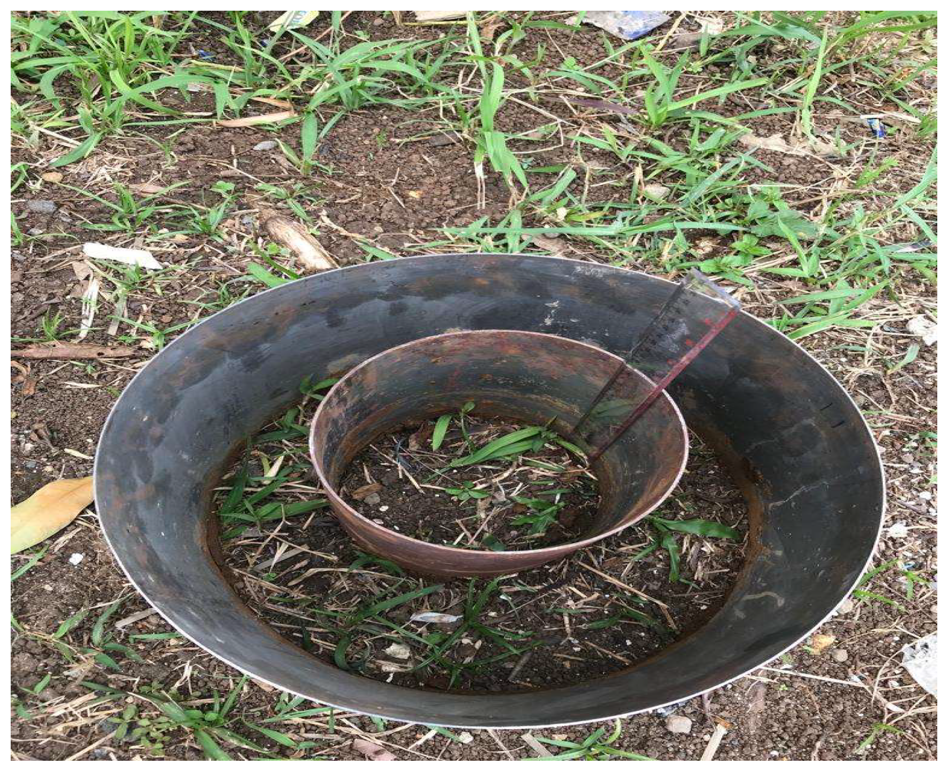
2.1. Study Area, Experimental Method and Data Collection
2.2. Infiltration Model
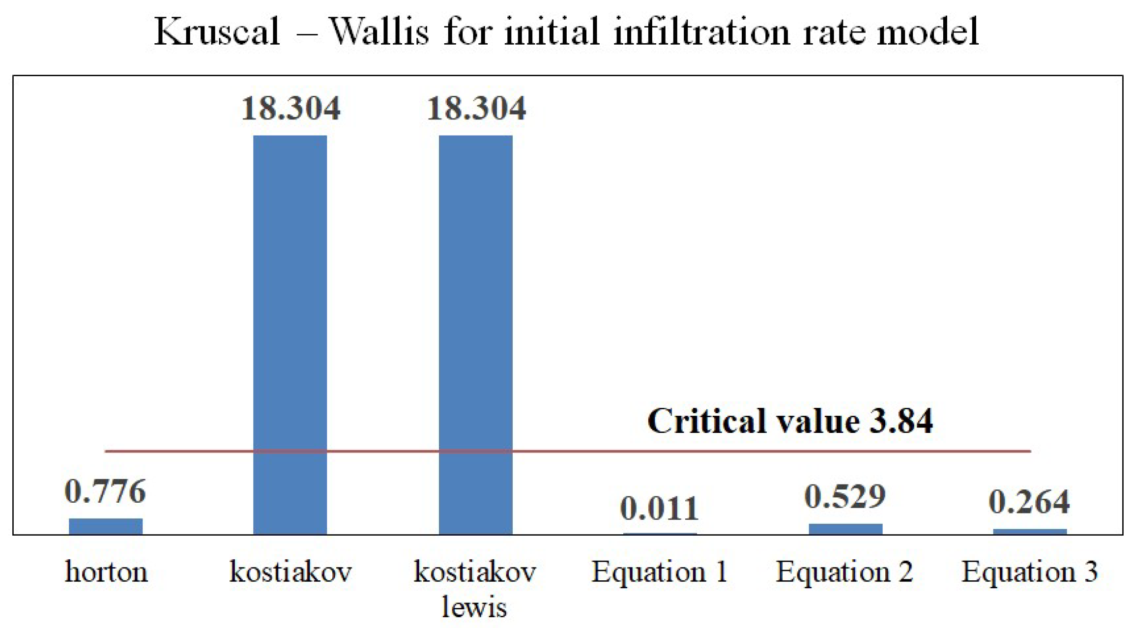
2.3. Evaluation of Best Infiltration Model
- A higher value of R2 represents a better fit of the model. R2 values of 0.7 < R2 < 1, 0.6 < R2 < 0.7, 0.5 < R2 < 0.6, and R2 < 0.5 were rated as very good, good, satisfactory, and unsatisfactory, respectively [32].
3. Results
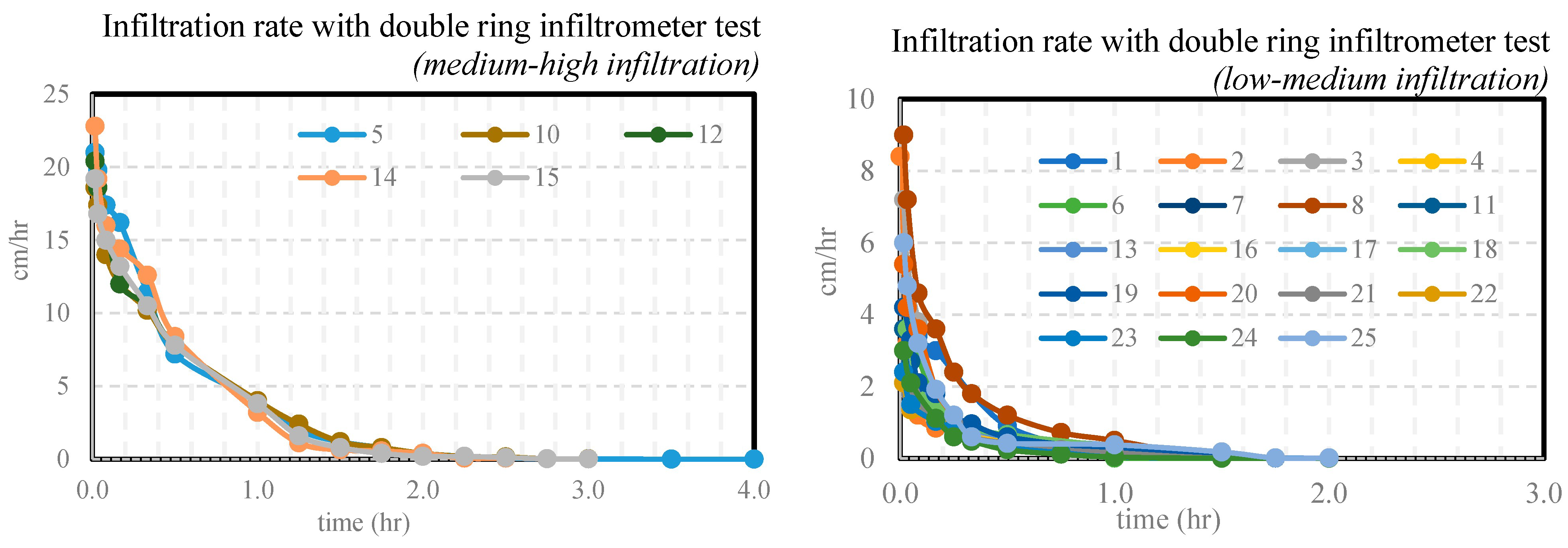
3.1. Observed Infiltration Rate Data
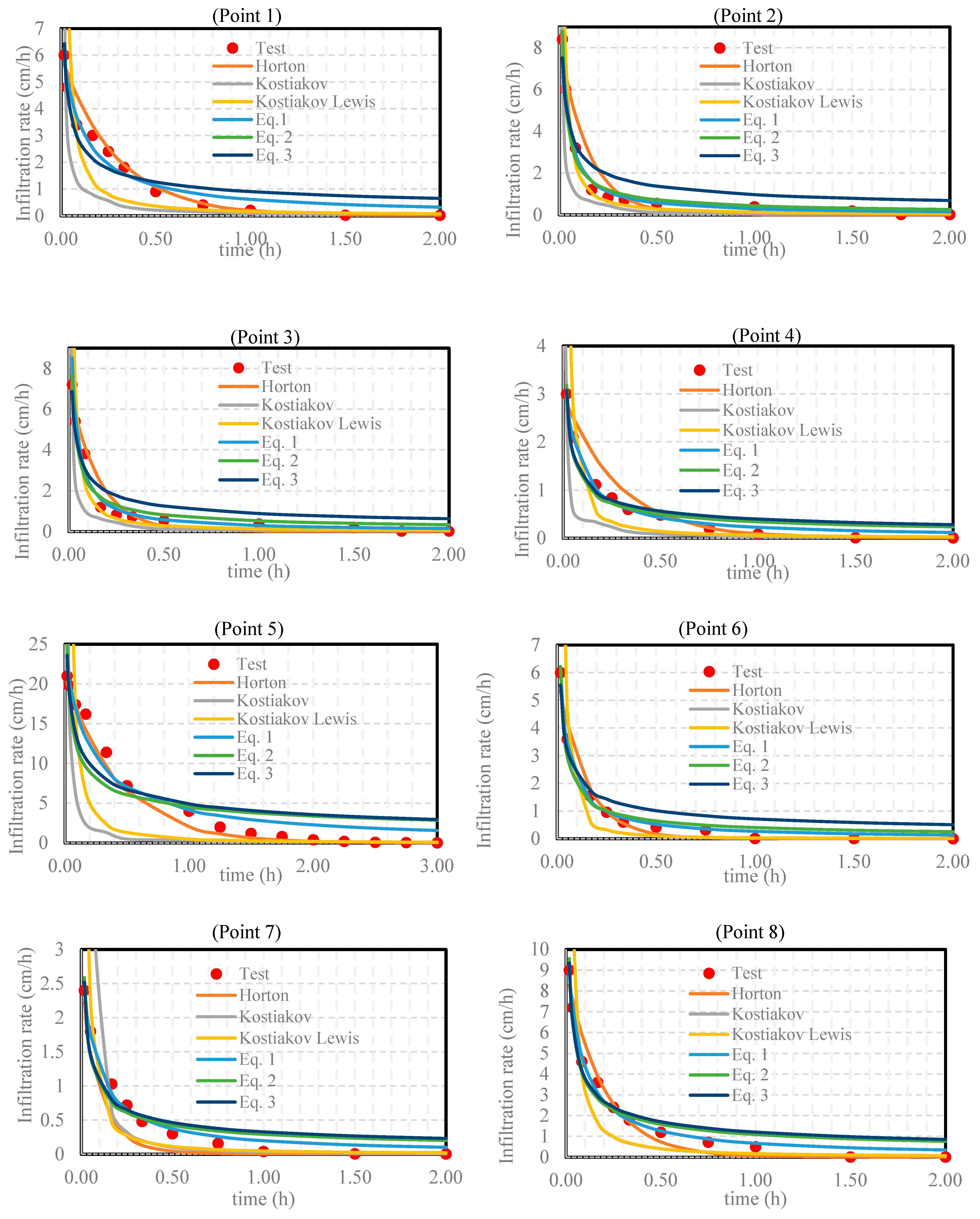
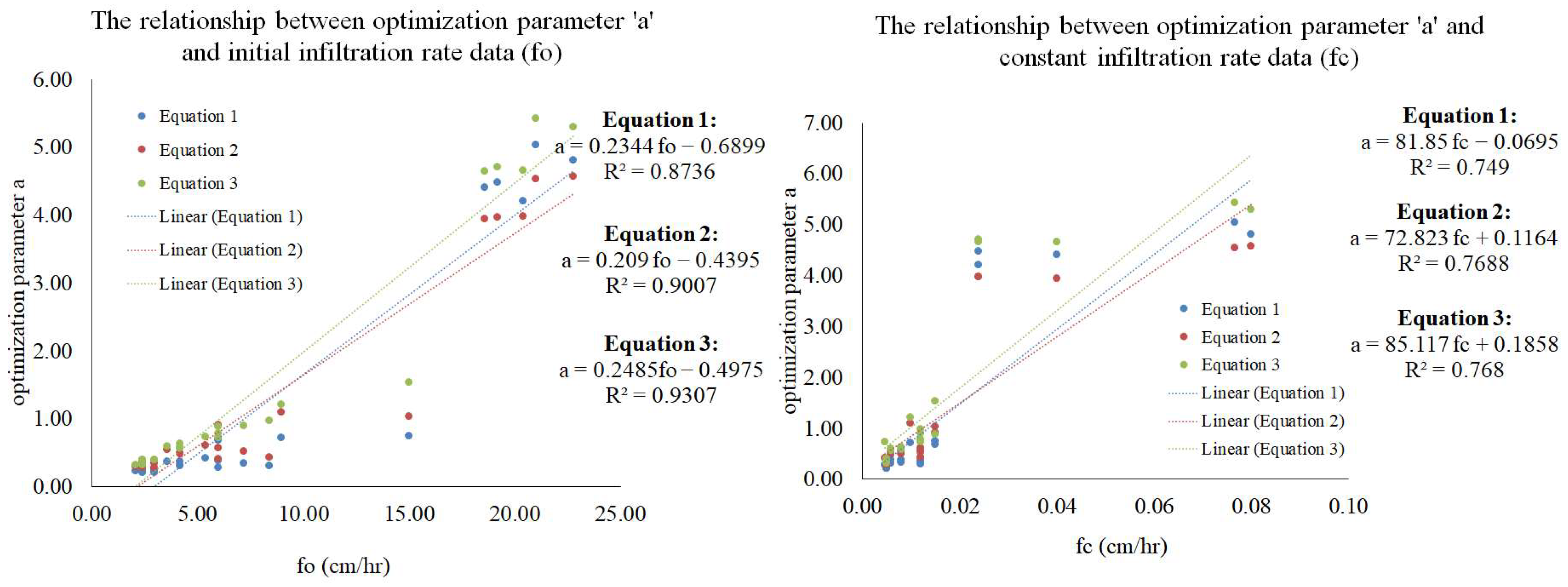
3.2. Infiltration Rate Model
4. Discussion
5. Conclusions
Author Contributions
Funding
Data Availability Statement
Acknowledgments
Conflicts of Interest
References
- Morbidelli, R.; Corradini, C.; Saltalippi, C.; Flammini, A.; Dari, J.; Govindaraju, R.S. Rainfall infiltration modeling: A review. Water 2018, 10, 1873. [Google Scholar] [CrossRef]
- Yang, M.; Zhang, Y.; Pan, X. Improving the Horton infiltration equation by considering soil moisture variation. J. Hydrol. 2020, 586, 124864. [Google Scholar] [CrossRef]
- Amami, R.; Ibrahimi, K.; Sher, F.; Milham, P.; Ghazouani, H.; Chehaibi, S.; Hussain, Z.; Iqbal, H.M.N. Impacts of different tillage practices on soil water infiltration for sustainable agriculture. Sustainability 2021, 13, 3155. [Google Scholar] [CrossRef]
- Moret-Fernández, D.; Latorre, B.; Lassabatere, L.; Di Prima, S.; Castellini, M.; Yilmaz, D.; Angulo-Jaramilo, R. Sequential infiltration analysis of infiltration curves measured with disc infiltrometer in layered soils. J. Hydrol. 2021, 600, 126542. [Google Scholar] [CrossRef]
- Panahi, M.; Khosravi, K.; Ahmad, S.; Panahi, S.; Heddam, S.; Melesse, A.M.; Omidvar, E.; Lee, C.-W. Cumulative infiltration and infiltration rate prediction using optimized deep learning algorithms: A study in Western Iran. J. Hydrol. Reg. Stud. 2021, 35, 100825. [Google Scholar] [CrossRef]
- Green, W.H.; Ampt, G.A. Studies on Soil Physics. J. Agric. Sci. 1911, 4, 1. [Google Scholar] [CrossRef]
- PHILIP, J.R. Theory of Infiltration; Academic Press, INC.: Cambridge, MA, USA, 1969; Volume 5. [Google Scholar]
- Kostiakov, A.N. On the dynamics of the coefficient of water percolation in soils and on the necessity of studying it from a dynamic point of view for purposes of amelioration. Trans. 6th Cong. Int. Soil Sci. Part A 1932, 17–21. [Google Scholar]
- Horton, R.E. The role of infiltration in the hydrology cycle. Trans. Am. Geophys. Union 1933, 14, 446–460. [Google Scholar]
- Mezencev, V.J. Theory of formation of the surface runoff. Meteorol. Hidrol. 1948, 3, 33–40. (In Russian) [Google Scholar]
- Ren, X.; Hong, N.; Li, L.; Kang, J.; Li, J. Effect of infiltration rate changes in urban soils on stormwater runoff process. Geoderma 2020, 363, 114158. [Google Scholar] [CrossRef]
- Bamutaze, Y.; Tenywa, M.M.; Majaliwa, M.J.G.; Vanacker, V.; Bagoora, F.; Magunda, M.; Obando, J.; Wasige, J.E. Infiltration characteristics of volcanic sloping soils on Mt. Elgon, Eastern Uganda. Catena 2010, 80, 122–130. [Google Scholar] [CrossRef]
- Swathi, V.; Raju, K.S.; Singh, A.P. Application of Storm Water Management Model to an Urban Catchment. In Hydrologic Modeling Select Proceedings of ICWEES-2016; Springer: Singapore, 2018; pp. 175–184. [Google Scholar] [CrossRef]
- Bayabil, H.K.; Dile, Y.T.; Tebebu, T.Y.; Engda, T.A.; Steenhuis, T.S. Evaluating infiltration models and pedotransfer functions: Implications for hydrologic modeling. Geoderma 2019, 338, 159–169. [Google Scholar] [CrossRef]
- Babaei, F.; Zolfaghari, A.A.; Yazdani, M.R.; Sadeghipour, A. Spatial analysis of infiltration in agricultural lands in arid areas of Iran. Catena 2018, 170, 25–35. [Google Scholar] [CrossRef]
- Lewis, M.R. The rate of infiltration of water in irrigation-practice. Trans. Am. Geophys. Union 1937, 18, 361–368. [Google Scholar] [CrossRef]
- Verma, S. Modified Horton’s infiltration equation. J. Hydrol. 1982, 58, 383–388. [Google Scholar] [CrossRef]
- Rossman, L.A. Storm Water Management Model User’s Manual Version 5.0. EPA/600/R-05/040. In Storm Water Management Model User’s Manual; United States Environmental Protection Agency: Cincinnati, OH, USA, 2010. [Google Scholar]
- Xin, Y.; Xie, Y.; Liu, Y. Effects of Residue Cover on Infiltration Process of the Black Soil Under Rainfall Simulations. Water 2019, 11, 2593. [Google Scholar] [CrossRef]
- Bergeson, C.B.; Martin, K.L.; Doll, B.; Cutts, B.B. Soil infiltration rates are underestimated by models in an urban watershed in central North Carolina, USA. J. Environ. Manag. 2022, 313, 115004. [Google Scholar] [CrossRef]
- Pachepsky, Y.; Karahan, G. On shapes of cumulative infiltration curves. Geoderma 2022, 412, 115715. [Google Scholar] [CrossRef]
- Komlos, J. Behavioral Indifference Curves. 2014. Available online: http://www.nber.org/papers/w20240 (accessed on 10 June 2014).
- Li, M.; Liu, T.; Duan, L.; Luo, Y.; Ma, L.; Wang, Y.; Zhou, Y.; Chen, Z. Scale transfer and simulation of the infiltration in chestnut soil in a semi-arid grassland basin. Ecol. Eng. 2020, 158, 106045. [Google Scholar] [CrossRef]
- Ruggenthaler, R.; Meißl, G.; Geitner, C.; Leitinger, G.; Endstrasser, N.; Schöberl, F. Investigating the impact of initial soil moisture conditions on total infiltration by using an adapted double-ring infiltrometer. Hydrol. Sci. J. 2016, 61, 1263–1279. [Google Scholar] [CrossRef]
- Warsi, T.; Kumar, V.S.; Dhakate, R.; Manikyamba, C.; Rao, T.V.; Rangarajan, R. An integrated study of electrical resistivity tomography and infiltration method in deciphering the characteristics and potentiality of unsaturated zone in crystalline rock. HydroResearch 2019, 2, 109–118. [Google Scholar] [CrossRef]
- ASTM-D3385–18; Infiltration Rate of Soils in Field Using Double Ring Infiltrometer. ASTM International: West Conshohocken, PA, USA, 2021; Volume I, pp. 1–8.
- Munawaroh, N.; Puspitasari, N.N.A.; Hadi, M.P.; Suarma, U. The comparison of rainfall intensity analysis methods in upstream area of Belik Watershed, Yogyakarta. IOP Conf. Ser. Earth Environ. Sci. 2020, 451, 012090. [Google Scholar] [CrossRef]
- Sherman, C.W. Frequency and Intensity of Excessive Rainfalls at Boston, Massachusetts. Trans. Am. Soc. Civ. Eng. 1931, 95, 951–960. [Google Scholar] [CrossRef]
- Khansa, P.; Sofiyah, E.S.; Suryawan, I.W.K. Determination of Rain Intensity Based on Rain Characteristics Observed from Rain Observation Stations Around South Jakarta. J. Adv. Civ. Environ. Eng. 2020, 3, 94–103. [Google Scholar] [CrossRef]
- Minh, H.V.T.; Lavane, K.; Lanh, L.T.; Thinh, L.V.; Cong, N.P.; Ty, T.V.; Downes, N.K.; Kumar, P. Developing Intensity-Duration-Frequency (IDF) Curves Based on Rainfall Cumulative Distribution Frequency (CDF) for Can Tho City, Vietnam. Earth 2022, 3, 866–880. [Google Scholar] [CrossRef]
- Atta-Darkwa, T.; Asare, A.; Amponsah, W.; Oppong, E.D.; Agbeshie, A.A.; Budu, M.; Larbi, I.; Akolgo, G.A.; Quaye, D.N.D. Performance evaluation of infiltration models under different tillage operations in a tropical climate. Sci. Afr. 2022, 17, e01318. [Google Scholar] [CrossRef]
- Moriasi, D.N.; Arnold, J.G.; van Liew, M.W.; Bingner, R.L.; Harmel, R.D.; Veith, T.L. Model Evaluation Guidelines for Systematic Quantification of Accuracy in Watershed Simulations. Trans. ASABE 2007, 50, 885–900. [Google Scholar] [CrossRef]
- Carlander, J.; Trygg, K.; Moshfegh, B. Integration of measurements and time diaries as complementary measures to improve resolution of BES. Energies 2019, 12, 2072. [Google Scholar] [CrossRef]
- Corrado, V.; Fabrizio, E. Steady-State and Dynamic Codes, Critical Review, Advantages and Disadvantages, Accuracy, and Reliability; Elsevier Inc.: Amsterdam, The Netherlands, 2018. [Google Scholar]
- Willmott, C.J. On the validation of models. Phys. Geogr. 1981, 2, 184–194. [Google Scholar] [CrossRef]
- Moges, D.M.; Virro, H.; Kmoch, A.; Cibin, R.; Rohith, A.; Martínez-Salvador, A.; Conesa-García, C.; Uuemaa, E. How does the choice of DEMs affect catchment hydrological modeling? Sci. Total Environ. 2023, 892, 164627. [Google Scholar] [CrossRef]
- Khai, W.J.; Sami, B.F.Z.; Fai, C.M.; Essam, Y.; Ahmed, A.N.; El-Shafie, A. Investigating the reliability of machine learning algorithms as a sustainable tool for total suspended solid prediction. Ain Shams Eng. J. 2021, 12, 1607–1622. [Google Scholar] [CrossRef]
- Mbuli, N.; Mendu, B.; Pretorius, J.-H.C. Statistical analysis of forced outage duration data for subtransmission circuit breakers. Energy Rep. 2022, 8, 1424–1433. [Google Scholar] [CrossRef]
- Janottama, S.Z.; Triana, K. Delineating the groundwater protection zone (GPZ) around a water supply plant in Bekasi, West Java, Indonesia. Groundw. Sustain. Dev. 2022, 17, 100762. [Google Scholar] [CrossRef]


| Point | Grid Location | Yearly Rainfall (mm) | Slope (%) | Land Use | Soil Texture |
|---|---|---|---|---|---|
| 1 | Pesantren Mina 90 | 3585 (very high) | 5.6 (flat to steep) | housing | loamy sand |
| 2 | Gunung Salak Endah | 3869 (very high) | 5.7 (flat to steep) | paddy field | sandy loam |
| 3 | Gunung Menir | 3869 (very high) | 8 (flat to steep) | paddy field | sandy loam |
| 4 | Cibungbulang | 3869 (very high) | 3 (flat) | housing | fine sandy loam |
| 5 | Cimandirasa | 3869 (very high) | 20 (steep) | forest | loamy sand |
| 6 | Leuwisadeng | 3869 (very high) | 5.8 (flat to steep) | paddy field | fine sandy loam |
| 7 | Ciheurang | 1572 (medium) | 2.3 (flat) | paddy field, shrubs | fine sandy loam |
| 8 | Babakan Encle | 3869 (very high) | 5.5 (flat to steep) | paddy field, shrubs | loamy sand |
| 9 | Purwasari | 3869 (very high) | 4 (flat) | paddy field | loamy sand |
| 10 | Leuweung | 3869 (very high) | 4 (flat) | plantation | loamy sand |
| 11 | Ciomas | 1572 (medium) | 2.5 (flat) | housing | loamy sand |
| 12 | Jami NFBS | 3869 (very high) | 6 (flat to steep) | plantation | loamy sand |
| 13 | Handeuleum | 3869 (very high) | 5.5 (flat to steep) | paddy field | fine sandy loam |
| 14 | Cianten | 3869 (very high) | 4.5 (flat) | plantation | loamy sand |
| 15 | Cijeruk | 3869 (very high) | 2.5 (flat) | plantation | loamy sand |
| 16 | Ciseeng | 1572 (medium) | 1.75 (flat) | paddy field | fine sandy loam |
| 17 | Gunung Sindur | 1572 (medium) | 3.5 (flat) | paddy field, shrubs | fine sandy loam |
| 18 | Karehkel | 1572 (medium) | 3.8 (flat) | paddy field | sandy loam |
| 19 | Rumpin | 1572 (medium) | 3 (flat) | plantation | sandy loam |
| 20 | Serpong | 2079 (high) | 2.75 (flat) | housing | sandy loam |
| 21 | Cisauk | 2079 (high) | 2.25 (flat) | housing | fine sandy loam |
| 22 | Karawaci | 1403 (medium) | 2.75 (flat) | housing | fine sandy loam |
| 23 | PAP Tangerang | 1403 (medium) | 1.5 (flat) | housing | fine sandy loam |
| 24 | Slapang | 1403 (medium) | 2.25 (flat) | housing | sandy loam |
| 25 | Gaga | 1683 (medium) | 1 (flat) | paddy field | sandy loam |
| Infiltration Model | Equation | Parameter and Coefficients |
|---|---|---|
| Horton | fc = constant/final infiltration rate (cm/h), fo = initial infiltration rate (cm/h), k = empirical coefficient | |
| Kostiakov | a and b are empirical parameters, t = experiment time (h) | |
| Kostiakov–Lewis | a and b are empirical parameters, fc = constant/final infiltration rate (cm/h), t = experiment time | |
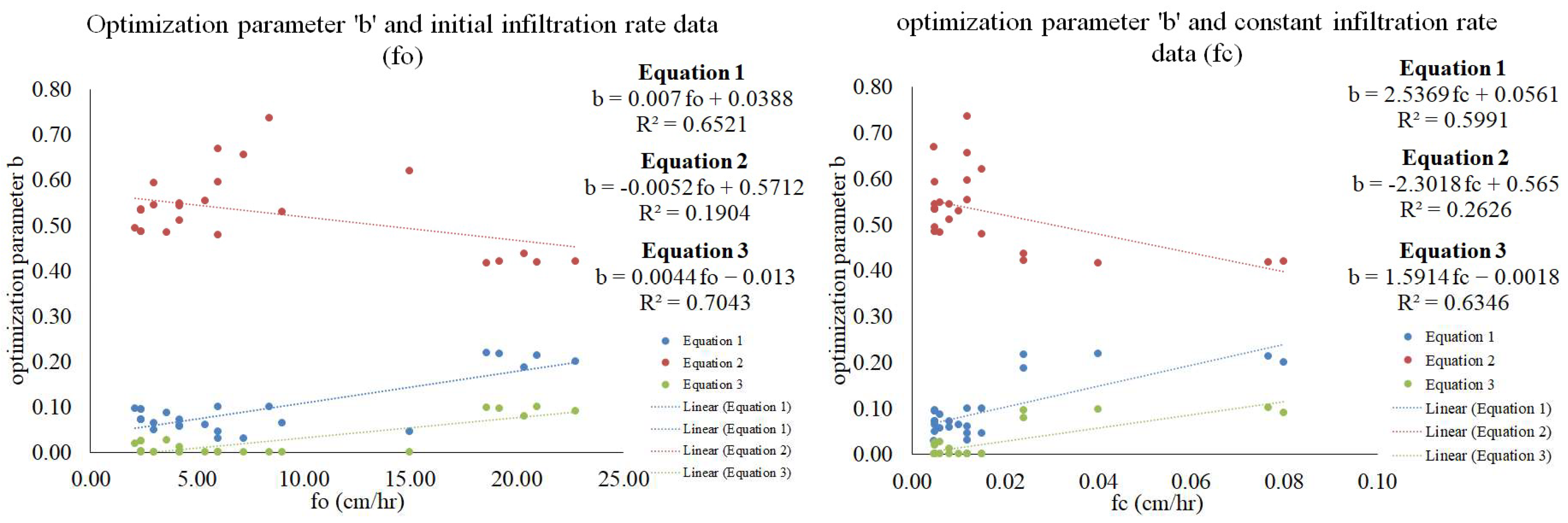
| Equation (1) | a and b are optimization parameters, t = experiment time (h) | |
| Equation (2) | a and b are optimization parameters, t = experiment time (h) | |
| Equation (3) | a and b are optimization parameters, t = experiment time (h) |
| Survey Point | Average Infiltration Rate (cm/h) | Initial Infiltration Rate (cm/h) | Constant Infiltration Rate (cm/h) | Survey Point | Average Infiltration Rate (cm/h) | Initial Infiltration Rate (cm/h) | Constant Infiltration Rate (cm/h) |
|---|---|---|---|---|---|---|---|
| 1 | 2.085 | 6.000 | 0.015 | 13 | 1.297 | 4.200 | 0.006 |
| 2 | 1.953 | 8.400 | 0.012 | 14 | 7.652 | 22.800 | 0.080 |
| 3 | 1.844 | 7.200 | 0.012 | 15 | 5.978 | 19.200 | 0.024 |
| 4 | 0.842 | 3.000 | 0.005 | 16 | 0.762 | 2.400 | 0.005 |
| 5 | 5.985 | 21.000 | 0.005 | 17 | 0.694 | 2.400 | 0.005 |
| 6 | 1.346 | 6.000 | 0.005 | 18 | 1.309 | 4.200 | 0.008 |
| 7 | 0.694 | 2.400 | 0.005 | 19 | 1.320 | 4.200 | 0.008 |
| 8 | 2.822 | 9.000 | 0.010 | 20 | 1.629 | 5.400 | 0.012 |
| 9 | 3.653 | 15.000 | 0.015 | 21 | 0.762 | 2.400 | 0.005 |
| 10 | 5.949 | 18.600 | 0.040 | 22 | 1.297 | 2.100 | 0.005 |
| 11 | 1.192 | 3.600 | 0.006 | 23 | 0.676 | 2.400 | 0.005 |
| 12 | 6.165 | 20.400 | 0.024 | 24 | 0.770 | 3.000 | 0.005 |
| 25 | 1.702 | 6.000 | 0.012 | ||||
| average rate (cm/h) | 2.384 | ||||||
| initial rate (cm/h) | 8.052 | ||||||
| constant rate (cm/h) | 0.015 | ||||||
| Point | Field Survey (cm/h) | Horton | Kostiakov, Kostiakov–Lewis | Equation (1) | Equation (2) | Equation (3) | |||||
|---|---|---|---|---|---|---|---|---|---|---|---|
| fo | fc | k | a | b | a | b | a | b | a | b | |
| 1 | 6.00 | 0.0150 | 3.459 | 0.149 | −1.208 | 0.68 | 0.10 | 0.91 | 0.48 | 0.88 | 0.000 |
| 2 | 8.40 | 0.0120 | 6.835 | 0.116 | −1.226 | 0.30 | 0.10 | 0.43 | 0.74 | 0.97 | 0.000 |
| 3 | 7.20 | 0.0120 | 6.557 | 0.118 | −1.209 | 0.34 | 0.03 | 0.52 | 0.66 | 0.89 | 0.000 |
| 4 | 3.00 | 0.0050 | 3.535 | 0.055 | −1.312 | 0.24 | 0.06 | 0.34 | 0.54 | 0.40 | 0.000 |
| 5 | 21.00 | 0.058 | 2.326 | 0.489 | −1.433 | 5.03 | 0.21 | 4.53 | 0.42 | 5.41 | 0.100 |
| 6 | 6.00 | 0.0047 | 7.149 | 0.032 | −1.673 | 0.28 | 0.03 | 0.40 | 0.67 | 0.72 | 0.000 |
| 7 | 2.40 | 0.0050 | 4.032 | 0.044 | −1.318 | 0.21 | 0.07 | 0.29 | 0.53 | 0.33 | 0.001 |
| 8 | 9.00 | 0.0100 | 5.030 | 0.165 | −1.290 | 0.71 | 0.06 | 1.10 | 0.53 | 1.21 | 0.000 |
| 9 | 15.00 | 0.0150 | 3.720 | 0.265 | −1.410 | 0.74 | 0.04 | 1.03 | 0.62 | 1.53 | 0.000 |
| 10 | 18.60 | 0.0400 | 2.014 | 0.887 | −1.085 | 4.40 | 0.22 | 3.94 | 0.42 | 4.65 | 0.098 |
| 11 | 3.60 | 0.0060 | 3.671 | 0.088 | −1.244 | 0.37 | 0.09 | 0.54 | 0.48 | 0.59 | 0.026 |
| 12 | 20.40 | 0.0240 | 2.303 | 0.667 | −1.214 | 4.20 | 0.19 | 3.97 | 0.44 | 4.65 | 0.078 |
| 13 | 4.20 | 0.0060 | 2.848 | 0.088 | −1.230 | 0.31 | 0.06 | 0.48 | 0.55 | 0.56 | 0.000 |
| 14 | 22.80 | 0.0800 | 2.252 | 0.870 | −1.237 | 4.80 | 0.20 | 4.57 | 0.42 | 5.29 | 0.090 |
| 15 | 19.20 | 0.0240 | 2.201 | 0.665 | −1.201 | 4.48 | 0.22 | 3.96 | 0.42 | 4.70 | 0.096 |
| 16 | 2.40 | 0.0050 | 2.812 | 0.063 | −1.222 | 0.26 | 0.09 | 0.35 | 0.49 | 0.38 | 0.024 |
| 17 | 2.40 | 0.0050 | 4.032 | 0.044 | −1.318 | 0.21 | 0.07 | 0.29 | 0.53 | 0.33 | 0.001 |
| 18 | 4.20 | 0.0080 | 2.838 | 0.097 | −1.197 | 0.32 | 0.06 | 0.49 | 0.54 | 0.57 | 0.000 |
| 19 | 4.20 | 0.0080 | 3.011 | 0.095 | −1.247 | 0.37 | 0.07 | 0.56 | 0.51 | 0.62 | 0.012 |
| 20 | 5.40 | 0.0120 | 5.778 | 0.870 | −1.237 | 0.42 | 0.06 | 0.60 | 0.55 | 0.72 | 0.000 |
| 21 | 2.40 | 0.0050 | 3.183 | 0.063 | −1.222 | 0.26 | 0.09 | 0.35 | 0.49 | 0.38 | 0.024 |
| 22 | 2.10 | 0.0050 | 3.909 | 0.045 | −1.277 | 0.23 | 0.10 | 0.29 | 0.49 | 0.32 | 0.018 |
| 23 | 2.40 | 0.0050 | 3.989 | 0.044 | −1.304 | 0.20 | 0.07 | 0.28 | 0.53 | 0.31 | 0.000 |
| 24 | 3.00 | 0.0050 | 4.557 | 0.040 | −1.381 | 0.20 | 0.05 | 0.28 | 0.59 | 0.38 | 0.000 |
| 25 | 6.00 | 0.0120 | 5.954 | 0.120 | −1.189 | 0.37 | 0.05 | 0.56 | 0.60 | 0.78 | 0.000 |
| Average | 8.05 | 0.01 | 3.92 | 0.25 | −1.28 | 1.20 | 0.10 | 1.24 | 0.53 | 1.50 | 0.023 |
| Maximum | 22.80 | 0.08 | 7.15 | 0.89 | −1.09 | 5.03 | 0.22 | 4.57 | 0.74 | 5.41 | 0.100 |
| Minimum | 2.10 | 0.00 | 2.01 | 0.03 | −1.67 | 0.20 | 0.03 | 0.28 | 0.42 | 0.31 | 0.000 |
| No | Infiltration Rate Equation | |||||
|---|---|---|---|---|---|---|
| Horton | Kostiakov | Kostiakov–Lewis | Equation (1) | Equation (2) | Equation (3) | |
| 1 | ||||||
| 2 | ||||||
| 3 | ||||||
| 4 | ||||||
| 5 | ||||||
| 6 | ||||||
| 7 | ||||||
| 8 | ||||||
| 9 | ||||||
| 10 | ||||||
| 11 | ||||||
| 12 | ||||||
| 13 | ||||||
| 14 | ||||||
| 15 | ||||||
| 16 | ||||||
| 17 | ||||||
| 18 | ||||||
| 19 | ||||||
| 20 | ||||||
| 21 | ||||||
| 22 | ||||||
| 23 | ||||||
| 24 | ||||||
| 25 | ||||||
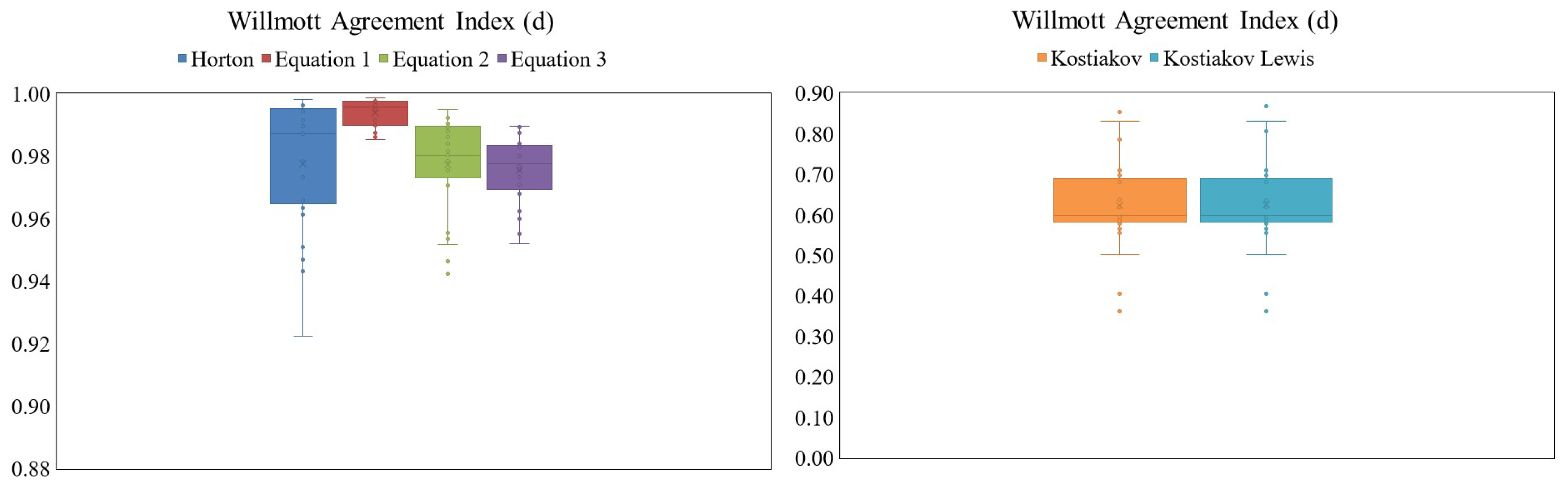
| Point | RMSE | R2 | ||||||||||
|---|---|---|---|---|---|---|---|---|---|---|---|---|
| Horton | Kostiakov | Kostiakov–Lewis | Equation (1) | Equation (2) | Equation (3) | Horton | Kostiakov | Kostiakov–Lewis | Equation (1) | Equation (2) | Equation (3) | |
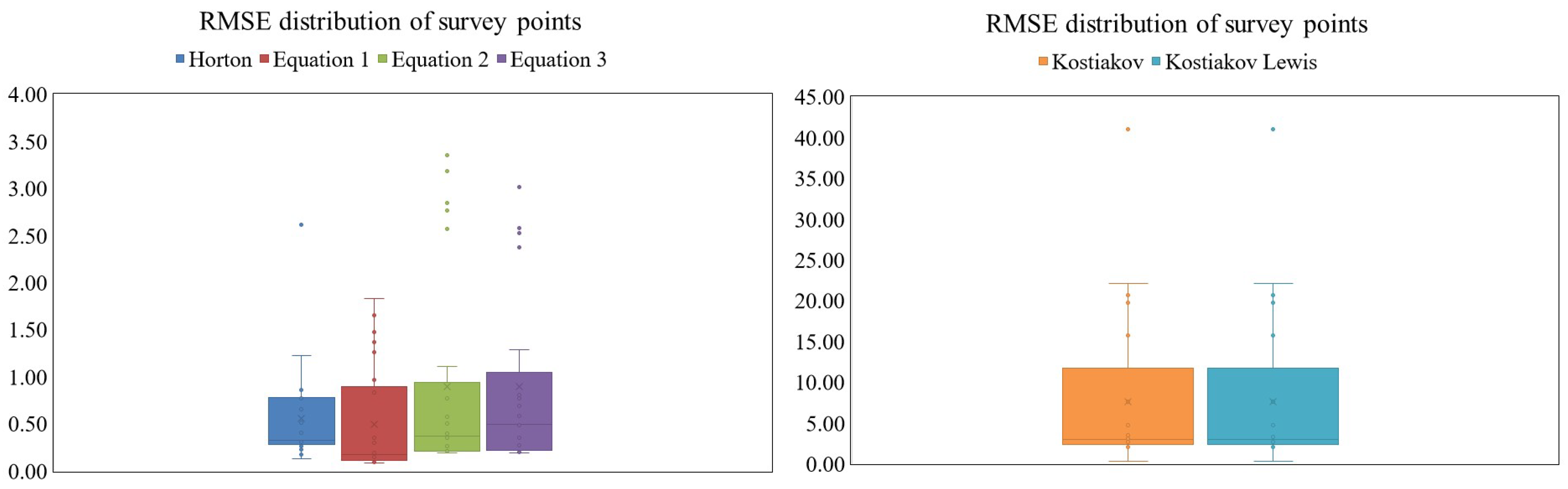
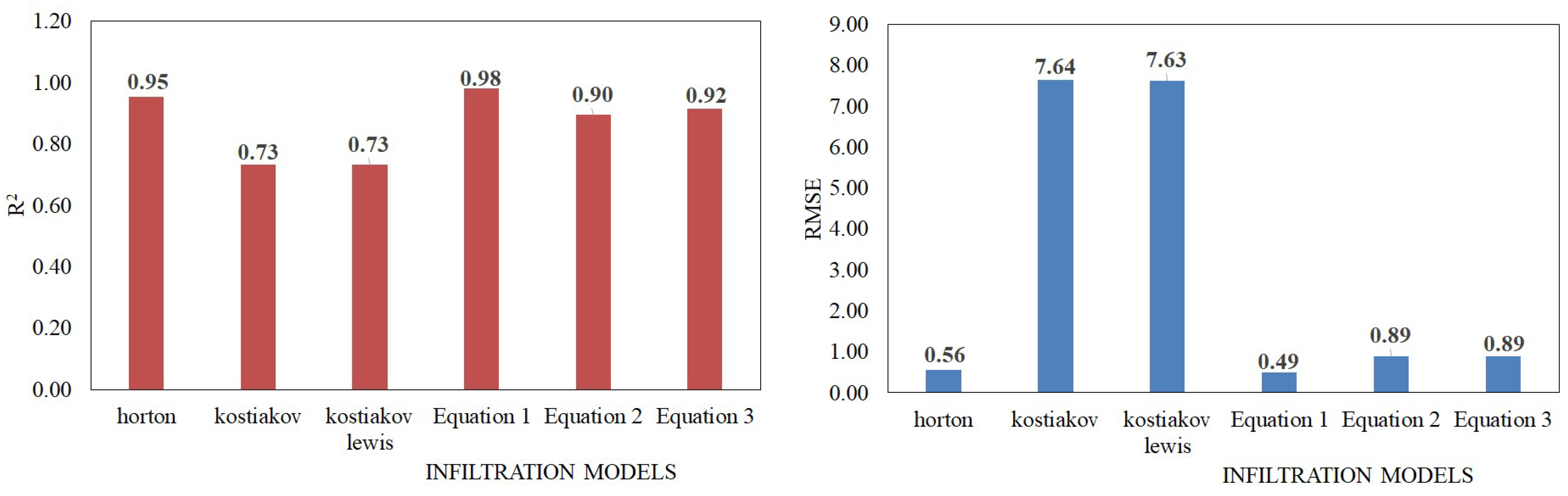
| 1 | 0.41 | 4.75 | 4.75 | 0.35 | 0.57 | 0.59 | 0.97 | 0.71 | 0.71 | 0.97 | 0.92 | 0.91 |
| 2 | 0.78 | 2.97 | 2.83 | 0.20 | 0.37 | 0.81 | 0.92 | 0.92 | 0.92 | 0.99 | 0.72 | 0.79 |
| 3 | 0.51 | 2.93 | 2.93 | 0.32 | 0.49 | 0.67 | 0.95 | 0.86 | 0.86 | 0.98 | 0.96 | 0.97 |
| 4 | 0.28 | 2.82 | 2.82 | 0.09 | 0.21 | 0.22 | 0.95 | 0.77 | 0.77 | 0.99 | 0.96 | 0.97 |
| 5 | 0.93 | 40.99 | 40.99 | 1.60 | 3.32 | 2.99 | 0.99 | 0.46 | 0.46 | 0.97 | 0.83 | 0.88 |
| 6 | 0.32 | 7.64 | 7.64 | 0.13 | 0.29 | 0.50 | 0.97 | 0.81 | 0.81 | 1.00 | 0.98 | 0.98 |
| 7 | 0.28 | 2.32 | 2.32 | 0.10 | 0.21 | 0.22 | 0.95 | 0.72 | 0.72 | 0.99 | 0.93 | 0.94 |
| 8 | 0.13 | 0.29 | 0.28 | 0.16 | 0.40 | 0.49 | 0.96 | 0.95 | 0.95 | 0.96 | 0.87 | 0.86 |
| 9 | 2.61 | 22.12 | 22.12 | 0.83 | 1.11 | 1.29 | 0.92 | 0.75 | 0.75 | 0.96 | 0.93 | 0.95 |
| 10 | 0.80 | 15.67 | 15.68 | 1.26 | 2.57 | 2.37 | 0.99 | 0.59 | 0.59 | 0.97 | 0.86 | 0.91 |
| 11 | 0.27 | 3.28 | 3.28 | 0.10 | 0.29 | 0.28 | 0.96 | 0.69 | 0.69 | 0.99 | 0.94 | 0.96 |
| 12 | 0.86 | 20.65 | 20.66 | 1.37 | 2.76 | 2.52 | 0.99 | 0.57 | 0.57 | 0.98 | 0.87 | 0.91 |
| 13 | 0.68 | 2.90 | 2.90 | 0.17 | 0.27 | 0.29 | 0.87 | 0.81 | 0.81 | 0.98 | 0.96 | 0.97 |
| 14 | 1.23 | 15.84 | 15.86 | 1.83 | 3.18 | 3.02 | 0.98 | 0.62 | 0.62 | 0.96 | 0.87 | 0.90 |
| 15 | 0.77 | 19.71 | 19.72 | 1.48 | 2.84 | 2.58 | 0.99 | 0.54 | 0.54 | 0.97 | 0.84 | 0.89 |
| 16 | 0.23 | 2.25 | 2.26 | 0.10 | 0.21 | 0.20 | 0.95 | 0.72 | 0.72 | 0.99 | 0.93 | 0.95 |
| 17 | 0.28 | 2.32 | 2.32 | 0.10 | 0.21 | 0.22 | 0.95 | 0.72 | 0.72 | 0.99 | 0.93 | 0.94 |
| 18 | 0.66 | 2.77 | 2.78 | 0.13 | 0.26 | 0.28 | 0.88 | 0.81 | 0.81 | 0.99 | 0.97 | 0.97 |
| 19 | 0.53 | 3.50 | 3.50 | 0.17 | 0.35 | 0.35 | 0.92 | 0.70 | 0.70 | 0.99 | 0.94 | 0.95 |
| 20 | 0.24 | 3.09 | 2.93 | 0.30 | 0.50 | 0.52 | 0.98 | 0.77 | 0.77 | 0.98 | 0.71 | 0.73 |
| 21 | 0.17 | 2.25 | 2.26 | 0.10 | 0.21 | 0.20 | 0.96 | 0.72 | 0.72 | 0.99 | 0.93 | 0.95 |
| 22 | 0.29 | 2.03 | 2.03 | 0.15 | 0.21 | 0.21 | 0.92 | 0.70 | 0.70 | 0.96 | 0.91 | 0.92 |
| 23 | 0.29 | 2.20 | 2.20 | 0.13 | 0.19 | 0.19 | 0.94 | 0.76 | 0.76 | 0.97 | 0.94 | 0.95 |
| 24 | 0.31 | 2.66 | 2.66 | 0.96 | 0.77 | 0.77 | 0.99 | 0.77 | 0.77 | 0.99 | 0.95 | 0.97 |
| 25 | 0.28 | 3.14 | 2.99 | 0.19 | 0.42 | 0.49 | 0.98 | 0.82 | 0.82 | 0.99 | 0.73 | 0.77 |
| Av | 0.57 | 7.64 | 7.63 | 0.49 | 0.89 | 0.89 | 0.95 | 0.73 | 0.73 | 0.98 | 0.90 | 0.92 |
| Max | 2.61 | 40.99 | 40.99 | 1.83 | 3.32 | 3.02 | 0.99 | 0.95 | 0.95 | 1.00 | 0.98 | 0.98 |
| Min | 0.13 | 0.29 | 0.28 | 0.09 | 0.19 | 0.19 | 0.87 | 0.46 | 0.46 | 0.96 | 0.71 | 0.73 |
Disclaimer/Publisher’s Note: The statements, opinions and data contained in all publications are solely those of the individual author(s) and contributor(s) and not of MDPI and/or the editor(s). MDPI and/or the editor(s) disclaim responsibility for any injury to people or property resulting from any ideas, methods, instructions or products referred to in the content. |
© 2023 by the authors. Licensee MDPI, Basel, Switzerland. This article is an open access article distributed under the terms and conditions of the Creative Commons Attribution (CC BY) license (https://creativecommons.org/licenses/by/4.0/).
Share and Cite
Hidayat, D.P.A.; Darsono, S.L.W.; Farid, M. Evaluation of Infiltration Modeling in the Cisadane Watershed in Indonesia: Existing and New Approach Equation. Water 2023, 15, 4149. https://doi.org/10.3390/w15234149
Hidayat DPA, Darsono SLW, Farid M. Evaluation of Infiltration Modeling in the Cisadane Watershed in Indonesia: Existing and New Approach Equation. Water. 2023; 15(23):4149. https://doi.org/10.3390/w15234149
Chicago/Turabian StyleHidayat, Dina P. A., Sri Legowo W. Darsono, and Mohammad Farid. 2023. "Evaluation of Infiltration Modeling in the Cisadane Watershed in Indonesia: Existing and New Approach Equation" Water 15, no. 23: 4149. https://doi.org/10.3390/w15234149
APA StyleHidayat, D. P. A., Darsono, S. L. W., & Farid, M. (2023). Evaluation of Infiltration Modeling in the Cisadane Watershed in Indonesia: Existing and New Approach Equation. Water, 15(23), 4149. https://doi.org/10.3390/w15234149