
The Criteria for Transition of Fluid to Nonlinear Flow for Fractured Rocks: The Role of Fracture Intersection and Aperture


Abstract
:1. Introduction
2. Governing Equations for Fluid Flow
2.1. Navier–Stokes Equations
2.2. Cubic Law
2.3. Forchheimer’s Equation
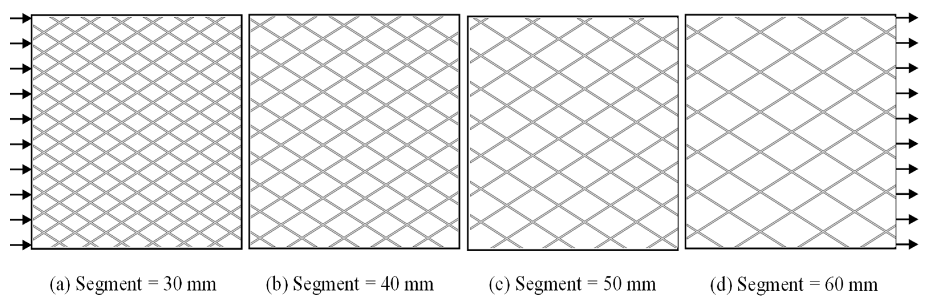
3. Geometric Modeling and Fluid Dynamic Computation
4. Simulation Results
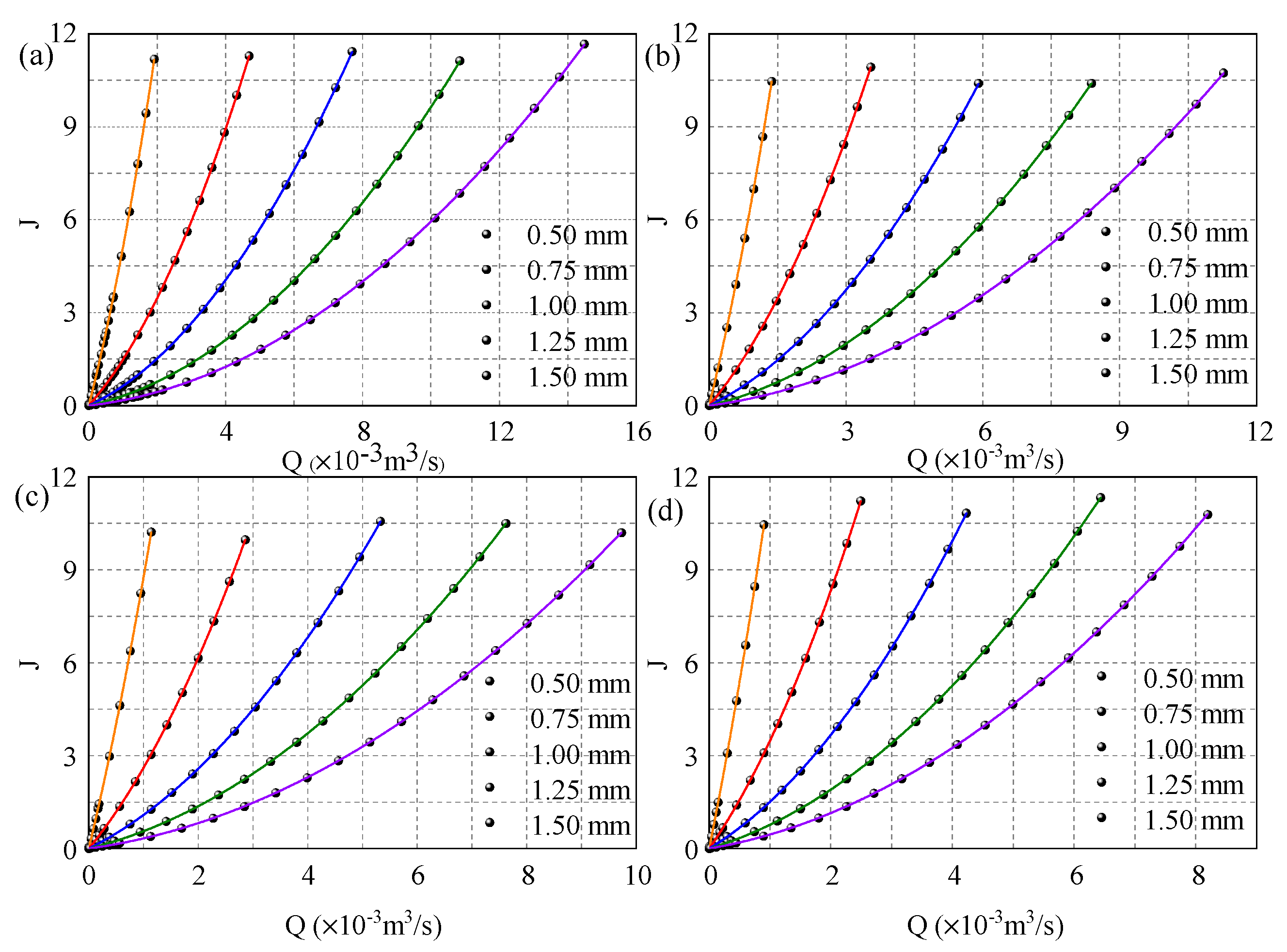
4.1. The Results of Fluid Dynamic Computation
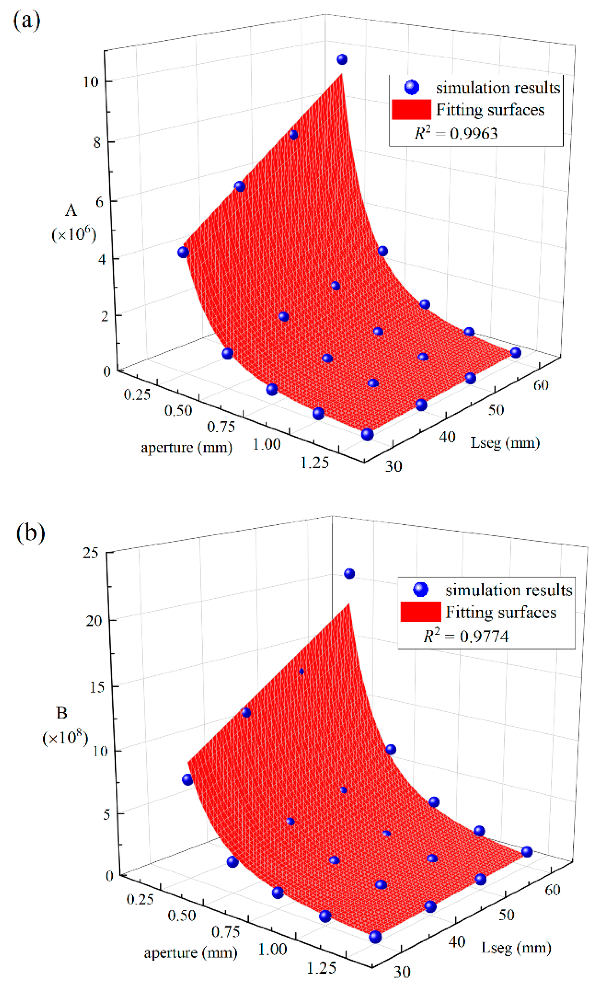
4.2. Effect of h on A and B under Different Lseg
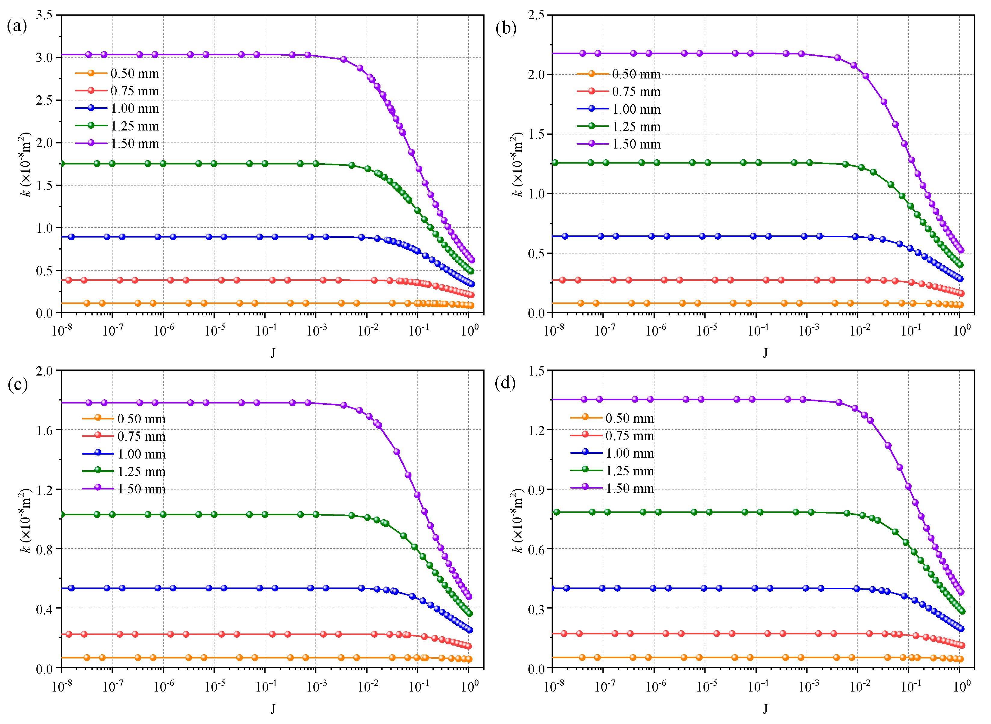
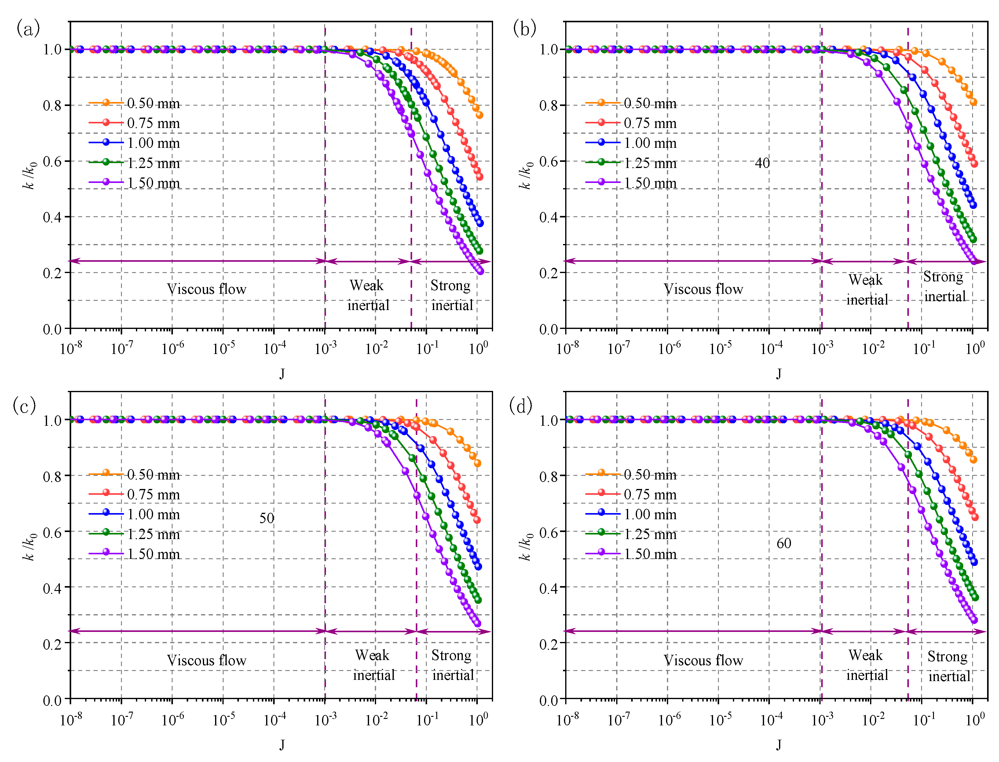
4.3. Effect of Hydraulic Gradient on Permeability k
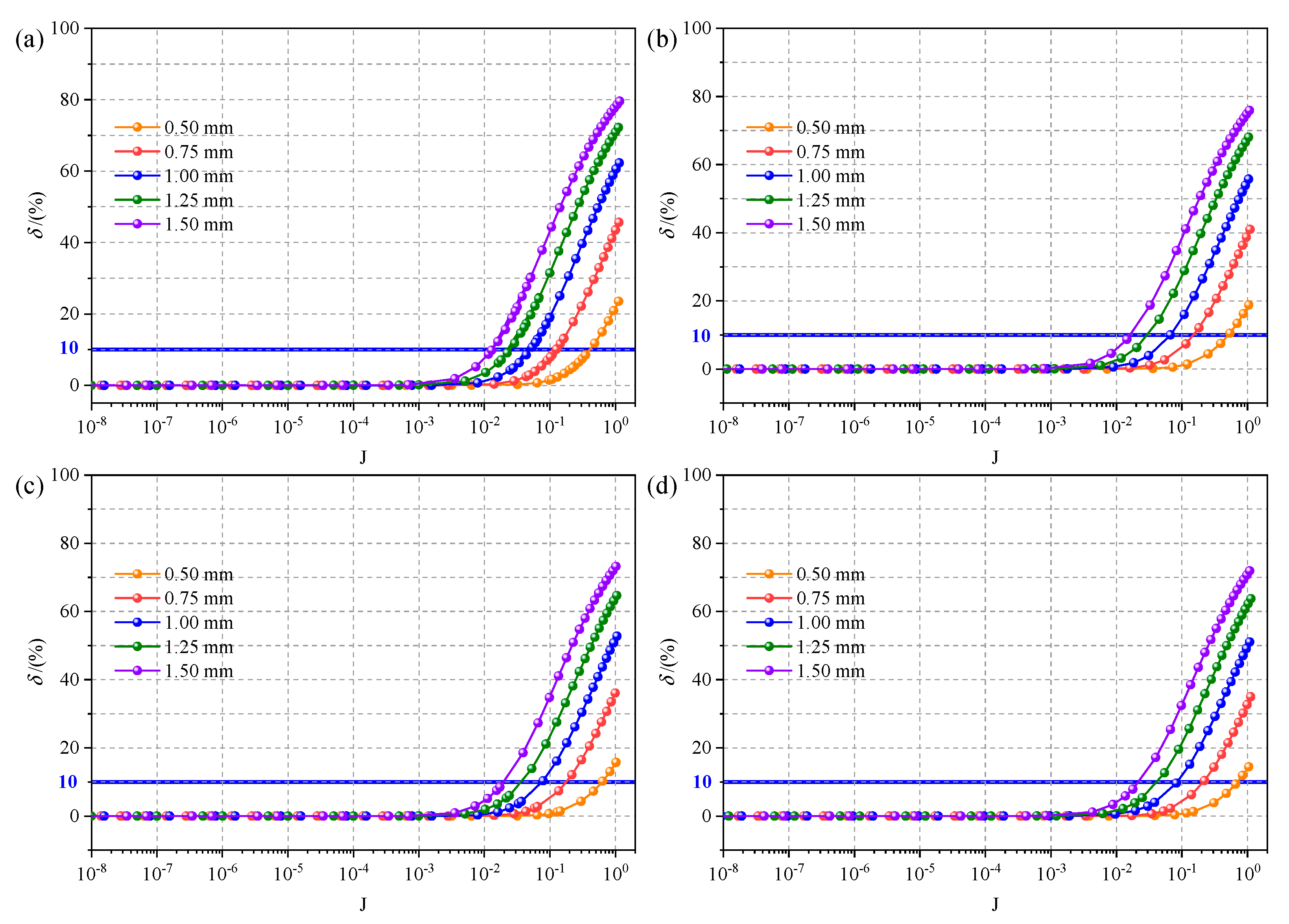
4.4. Effect of Hydraulic Gradient on Permeability Deviation
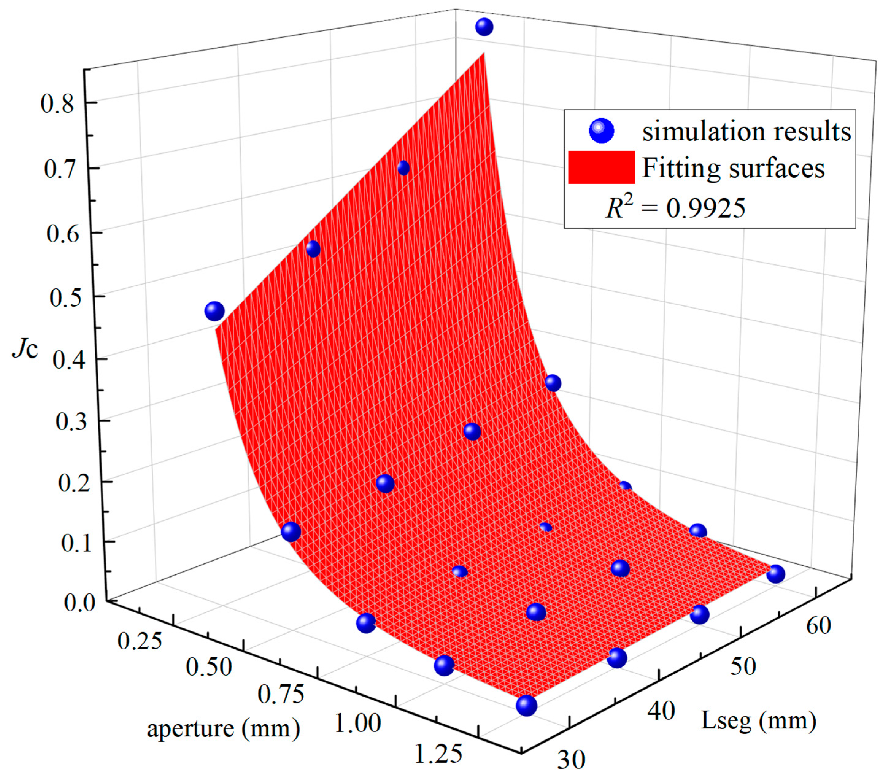
4.5. A Prediction Model for
5. The Application of Prediction Formulas for A, B, and
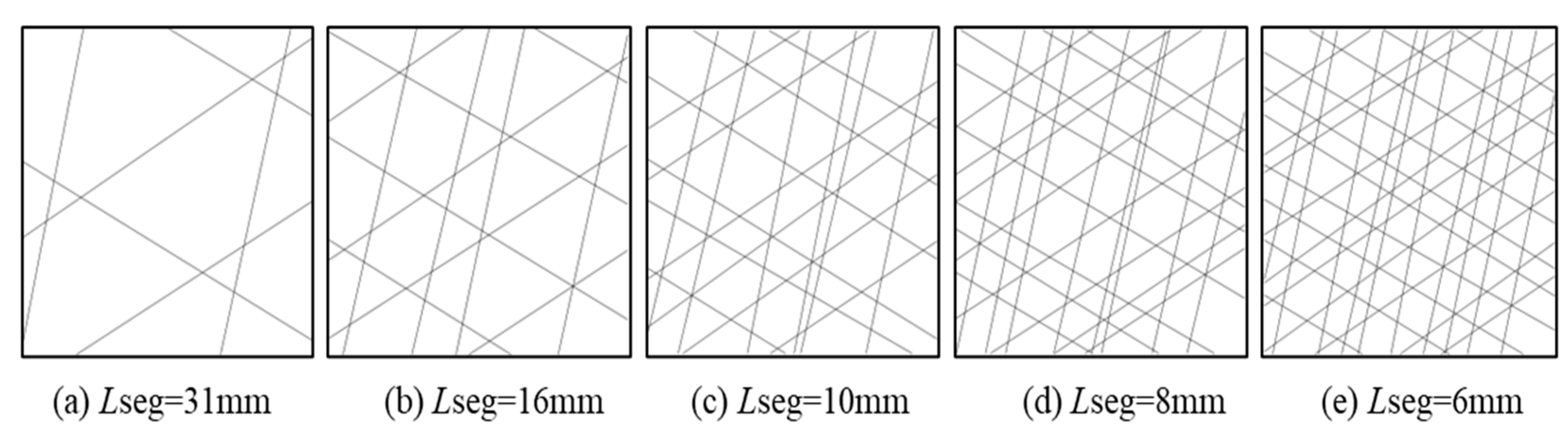
5.1. Generation of DFNs
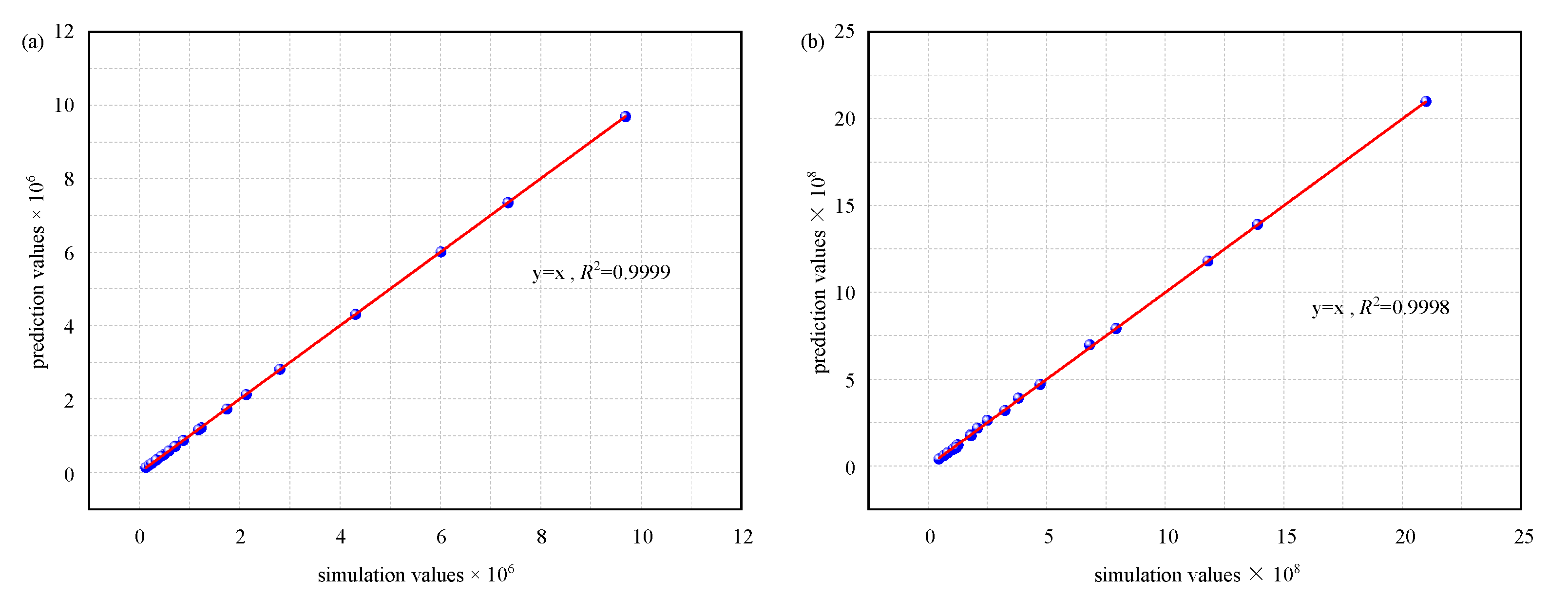
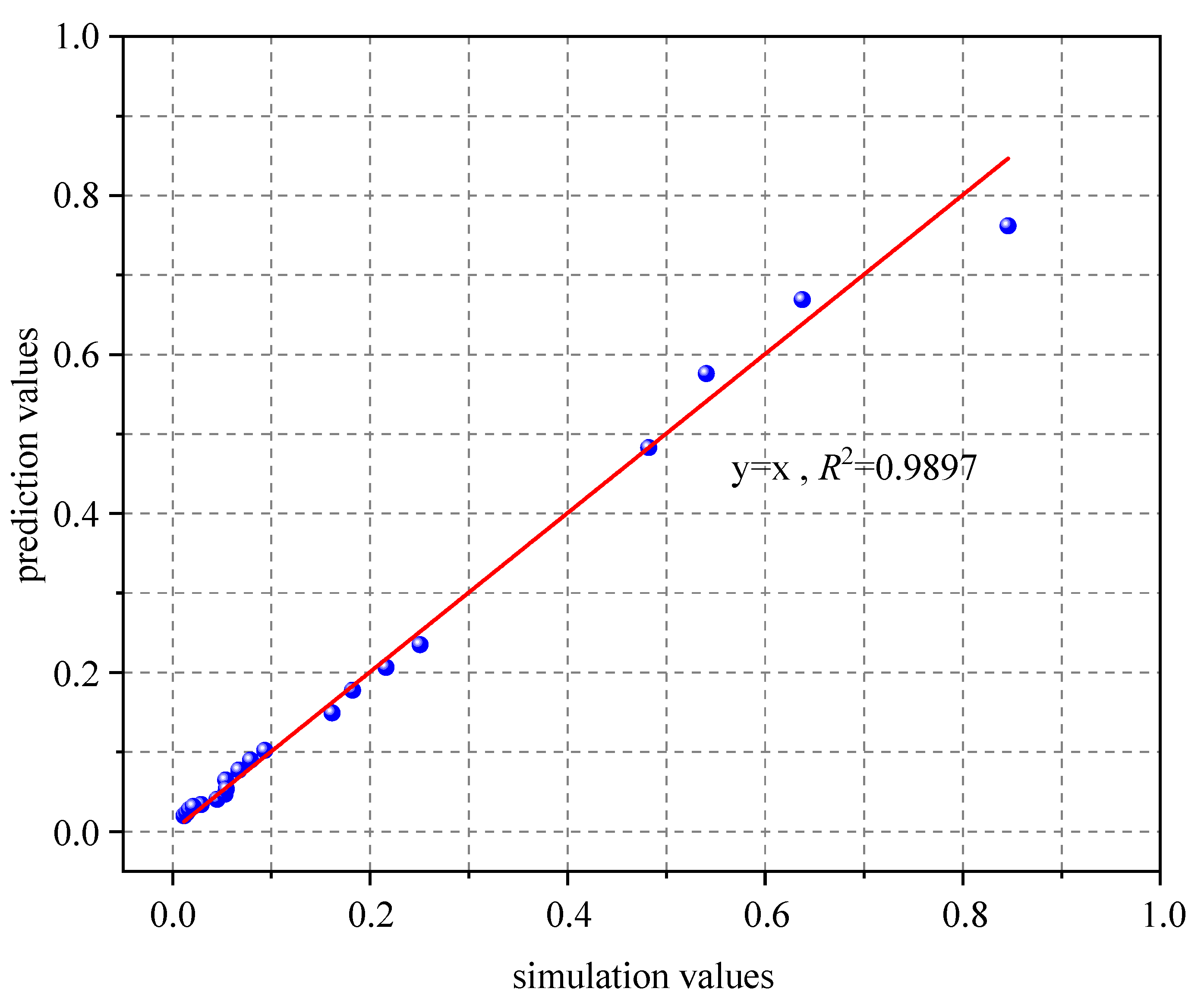
5.2. Comparison of Results of Fluid Dynamic Computation and Prediction Model
6. Conclusions
- (1)
- When a lower hydraulic gradient is applied to the DFN model, the fluid flow conforms to laminar flow. The flow rate is linearly correlated with the hydraulic gradient , which ensures that the permeability k remains constant. The permeability of fractured rocks can be accurately estimated by the cubic law.
- (2)
- With the increase in hydraulic gradient, the flow flux variance nonlinearly changes with the evolution of the hydraulic gradient. The permeability k sharply decreases with the increase in the hydraulic gradient, and the cubic law is not suitable for the computation of fluid flow through DFN models because the permeability deviation caused by the pressure loss would be underestimated.
- (3)
- With the increase in fracture aperture or the decrease in segment length, the fluid flow transition from the linear regime to the nonlinear regime in DFN models would occur at a lower . Therefore, a critical hydraulic gradient is proposed, below which the cubic law can be used to compute fluid flow through DFN models and above which Forchheimer’s law should be applied.
- (4)
- Mathematical expressions for prediction coefficients A and B and critical hydraulic gradient are proposed using a multiple regression algorithm. To verify the reliability of the proposed expressions, a set of discrete fracture network modes with well-known geometric distributions are generated. The coefficients A, B, and critical hydraulic gradient of these models are calculated through fluid dynamic computation and prediction models, and a correlation coefficient larger than 0.9 shows that the prediction model can provide a reasonable prediction of A, B, and .
Author Contributions
Funding
Data Availability Statement
Conflicts of Interest
References
- Rong, G.; Yang, J.; Cheng, L.; Zhou, C. Laboratory investigation of nonlinear flow characteristics in rough fractures during shear process. J. Hydrol. 2016, 541, 1385–1394. [Google Scholar] [CrossRef]
- Berre, I.; Doster, F.; Keilegavlen, E. Flow in Fractured Porous Media: A Review of Conceptual Models and Discretization Approaches. Transp. Porous Media 2018, 130, 215–236. [Google Scholar] [CrossRef]
- Zhao, Z.; Li, B.; Jiang, Y. Effects of Fracture Surface Roughness on Macroscopic Fluid Flow and Solute Transport in Fracture Networks. Rock Mech. Rock Eng. 2014, 47, 2279–2286. [Google Scholar] [CrossRef]
- Rivett, M.O.; Ellis, P.A.; Mackay, R. Urban groundwater baseflow influence upon inorganic river-water quality: The River Tame headwaters catchment in the City of Birmingham, UK. J. Hydrol. 2011, 400, 206–222. [Google Scholar] [CrossRef]
- Zhang, J.; Li, X.; Qin, Q.; Wang, Y.; Gao, X. Study on overlying strata movement patterns and mechanisms in super-large mining height stopes. Bull. Eng. Geol. Environ. 2023, 82, 142. [Google Scholar] [CrossRef]
- Shao, S.; Gao, C.; Guo, X.; Wang, Y.; Zhang, Z.; Yu, L.; Tang, H. Mapping the contaminant plume of an abandoned hydrocarbon disposal site with geophysical and geochemical methods, Jiangsu, China. Environ. Sci. Pollut. Res. 2019, 26, 24645–24657. [Google Scholar] [CrossRef]
- Ashraf, M.A.; Yusoff, I.; Yusof, M.; Alias, Y. Study of contaminant transport at an open-tipping waste disposal site. Environ. Sci. Pollut. Res. 2013, 20, 4689–4710. [Google Scholar] [CrossRef]
- Siddiqua, A.; Hahladakis, J.N.; Al-Attiya, W. An overview of the environmental pollution and health effects associated with waste landfilling and open dumping. Environ. Sci. Pollut. Res. 2022, 29, 58514–58536. [Google Scholar] [CrossRef]
- Liu, S.; Li, X. Experimental study on the effect of cold soaking with liquid nitrogen on the coal chemical and microstructural characteristics. Environ. Sci. Pollut. Res. 2022, 30, 36080–36097. [Google Scholar] [CrossRef]
- Karra, S.; Makedonska, N.; Viswanathan, H.S.; Painter, S.L.; Hyman, J.D. Effect of advective flow in fractures and matrix diffusion on natural gas production. Water Resour. Res. 2015, 51, 8646–8657. [Google Scholar] [CrossRef]
- Yang, T.; Jia, P.; Shi, W.; Wang, P.; Liu, H.; Yu, Q. Seepage–stress coupled analysis on anisotropic characteristics of the fractured rock mass around roadway. Tunn. Undergr. Space Technol. 2014, 43, 11–19. [Google Scholar] [CrossRef]
- Noorian Bidgoli, M.; Jing, L. Water Pressure Effects on Strength and Deformability of Fractured Rocks Under Low Confining Pressures. Rock Mech. Rock Eng. 2015, 48, 971–985. [Google Scholar] [CrossRef]
- Liu, S.; Sun, H.; Zhang, D.; Yang, K.; Li, X.; Wang, D.; Li, Y. Experimental study of effect of liquid nitrogen cold soaking on coal pore structure and fractal characteristics. Energy 2023, 275, 127470. [Google Scholar] [CrossRef]
- Li, H.; Li, X.; Fu, J.; Zhu, N.; Chen, D.; Wang, Y.; Ding, S. Experimental study on compressive behavior and failure characteristics of imitation steel fiber concrete under uniaxial load. Constr. Build. Mater. 2023, 399, 132599. [Google Scholar] [CrossRef]
- Nie, Z.; Chen, J.; Zhang, W.; Tan, C.; Ma, Z.; Wang, F.; Zhang, Y.; Que, J. A New Method for Three-Dimensional Fracture Network Modelling for Trace Data Collected in a Large Sampling Window. Rock Mech. Rock Eng. 2019, 53, 1145–1161. [Google Scholar] [CrossRef]
- Xue, K.; Zhang, Z.; Jiang, Y.; Luo, Y. Estimating the permeability of fractured rocks using topological characteristics of fracture network. Comput. Geotech. 2023, 157, 105337. [Google Scholar] [CrossRef]
- Konzuk, J.S.; Kueper, B.H. Evaluation of cubic law based models describing single-phase flow through a rough-walled fracture. Water Resour. Res. 2004, 40. [Google Scholar] [CrossRef]
- Xue, K.; Zhang, Z.; Zhong, C.; Jiang, Y.; Geng, X. A fast numerical method and optimization of 3D discrete fracture network considering fracture aperture heterogeneity. Adv. Water Resour. 2022, 162, 104164. [Google Scholar] [CrossRef]
- Hyman, J.D.; Karra, S.; Makedonska, N.; Gable, C.W.; Painter, S.L.; Viswanathan, H.S. dfnWorks: A discrete fracture network framework for modeling subsurface flow and transport. Comput. Geosci. 2015, 84, 10–19. [Google Scholar] [CrossRef]
- Brush, D.J.; Thomson, N.R. Fluid flow in synthetic rough-walled fractures: Navier-Stokes, Stokes, and local cubic law simulations. Water Resour. Res. 2003, 39. [Google Scholar] [CrossRef]
- Li, Q.; Han, Y.; Liu, X.; Ansari, U.; Cheng, Y.; Yan, C. Hydrate as a by-product in CO2 leakage during the long-term sub-seabed sequestration and its role in preventing further leakage. Environ. Sci. Pollut. Res. 2022, 29, 77737–77754. [Google Scholar] [CrossRef] [PubMed]
- Li, Q.; Wang, F.; Wang, Y.; Forson, K.; Cao, L.; Zhang, C.; Zhou, C.; Zhao, B.; Chen, J. Experimental investigation on the high-pressure sand suspension and adsorption capacity of guar gum fracturing fluid in low-permeability shale reservoirs: Factor analysis and mechanism disclosure. Environ. Sci. Pollut. Res. 2022, 29, 53050–53062. [Google Scholar] [CrossRef] [PubMed]
- Wang, F.; Xiao, Z.; Liu, X.; Ren, J.; Xing, T.; Li, Z.; Li, X.; Chen, Y. Strategic design of cellulose nanofibers@ zeolitic imidazolate frameworks derived mesoporous carbon-supported nanoscale CoFe2O4/CoFe hybrid composition as trifunctional electrocatalyst for Zn-air battery and self-powered overall water-splitting. J. Power Sources 2022, 521, 230925. [Google Scholar] [CrossRef]
- Javadi, M.; Sharifzadeh, M.; Shahriar, K.; Mitani, Y. Critical Reynolds number for nonlinear flow through rough-walled fractures: The role of shear processes. Water Resour. Res. 2014, 50, 1789–1804. [Google Scholar] [CrossRef]
- Nicholl, M.J.; Rajaram, H.; Glass, R.J.; Detwiler, R. Saturated flow in a single fracture: Evaluation of the Reynolds Equation in measured aperture fields. Water Resour. Res. 1999, 35, 3361–3373. [Google Scholar] [CrossRef]
- Oron, A.P.; Berkowitz, B. Flow in rock fractures: The local cubic law assumption reexamined. Water Resour. Res. 1998, 34, 2811–2825. [Google Scholar] [CrossRef]
- Zhang, Z.; Nemcik, J. Fluid flow regimes and nonlinear flow characteristics in deformable rock fractures. J. Hydrol. 2013, 477, 139–151. [Google Scholar] [CrossRef]
- Wang, M.; Chen, Y.-F.; Ma, G.-W.; Zhou, J.-Q.; Zhou, C.-B. Influence of surface roughness on nonlinear flow behaviors in 3D self-affine rough fractures: Lattice Boltzmann simulations. Adv. Water Resour. 2016, 96, 373–388. [Google Scholar] [CrossRef]
- Wang, Z.; Xu, C.; Dowd, P.; Xiong, F.; Wang, H. A Nonlinear Version of the Reynolds Equation for Flow in Rock Fractures With Complex Void Geometries. Water Resour. Res. 2020, 56. [Google Scholar] [CrossRef]
- Cunningham, D.; Auradou, H.; Shojaei-Zadeh, S.; Drazer, G. The Effect of Fracture Roughness on the Onset of Nonlinear Flow. Water Resour. Res. 2020, 56. [Google Scholar] [CrossRef]
- Zhang, Z.; Nemcik, J.; Ma, S. Micro- and macro-behaviour of fluid flow through rock fractures: An experimental study. Hydrogeol. J. 2013, 21, 1717–1729. [Google Scholar] [CrossRef]
- Jafari, A.; Babadagli, T. Estimation of equivalent fracture network permeability using fractal and statistical network properties. J. Pet. Sci. Eng. 2012, 92–93, 110–123. [Google Scholar] [CrossRef]
- Xue, K.; Zhang, Z.; Hao, S.; Luo, P.; Wang, Y. On the onset of nonlinear fluid flow transition in rock fracture network: Theoretical and computational fluid dynamic investigation. Phys. Fluids 2022, 34, 125114. [Google Scholar] [CrossRef]
- Kangsheng, X.; Zhenyu, Z.; Xuefeng, H.; Wenfeng, G. A fractal model for estimating the permeability of tortuous fracture networks with correlated fracture length and aperture. Phys. Fluids 2023, 35, 043615. [Google Scholar]
- Ranjith, P.G.; Darlington, W. Nonlinear single-phase flow in real rock joints. Water Resour. Res. 2007, 43, 146–156. [Google Scholar] [CrossRef]
- Li, B.; Liu, R.; Jiang, Y. Influences of hydraulic gradient, surface roughness, intersecting angle, and scale effect on nonlinear flow behavior at single fracture intersections. J. Hydrol. 2016, 538, 440–453. [Google Scholar] [CrossRef]
- Mahjour, S.K.; Faroughi, S.A. Selecting representative geological realizations to model subsurface CO2 storage under uncertainty. Int. J. Greenh. Gas Control. 2023, 127, 103920. [Google Scholar] [CrossRef]
- Soltanmohammadi, R.; Iraji, S.; de Almeida, T.R.; Munoz, E.R.; Vidal, A.C. Upscaling Challenges of Heterogeneous Carbonate Rocks: A Case Study of Brazilian Pre-Salt Analogous. In Proceedings of the Third EAGE Conference on Pre Salt Reservoirs, Rio de Janeiro, Brazil, 23–25 November 2022; European Association of Geoscientists & Engineers: Utrecht, The Netherlands, 2022; Volume 2022, pp. 1–6. [Google Scholar]
- Zhou, J.-Q.; Hu, S.-H.; Fang, S.; Chen, Y.-F.; Zhou, C.-B. Nonlinear flow behavior at low Reynolds numbers through rough-walled fractures subjected to normal compressive loading. Int. J. Rock Mech. Min. Sci. 2015, 80, 202–218. [Google Scholar] [CrossRef]
- Xiong, F.; Wei, W.; Xu, C.; Jiang, Q. Experimental and numerical investigation on nonlinear flow behaviour through three dimensional fracture intersections and fracture networks. Comput. Geotech. 2020, 121, 103446. [Google Scholar] [CrossRef]
- Xu, W.; Zhang, Y.; Li, X.; Wang, X.; Zhang, P. Study on three-dimensional fracture network connectivity path of rock mass and seepage characteristics based on equivalent pipe network. Environ. Earth Sci. 2019, 78, 1–21. [Google Scholar] [CrossRef]
- Liu, J.; Wang, Z.; Qiao, L.; Guo, J.; Li, W. Nonlinear Flow Model for Rock Fracture Intersections: The Roles of the Intersecting Angle, Aperture and Fracture Roughness. Rock Mech. Rock Eng. 2022, 55, 2385–2405. [Google Scholar] [CrossRef]
- Caulk, R.A.; Ghazanfari, E.; Perdrial, J.N.; Perdrial, N. Experimental investigation of fracture aperture and permeability change within Enhanced Geothermal Systems. Geothermics 2016, 62, 12–21. [Google Scholar] [CrossRef]
- Xiong, F.; Jiang, Q.; Xu, C.; Zhang, X.; Zhang, Q. Influences of connectivity and conductivity on nonlinear flow behaviours through three-dimension discrete fracture networks. Comput. Geotech. 2018, 107, 128–141. [Google Scholar] [CrossRef]
- Zhang, A.; Yang, J.; Cheng, L.; Ma, C. A simulation study on stress-seepage characteristics of 3D rough single fracture based on fluid-structure interaction. J. Pet. Sci. Eng. 2022, 211, 110215. [Google Scholar] [CrossRef]
- Ju, Y.; Dong, J.; Gao, F.; Wang, J. Evaluation of water permeability of rough fractures based on a self-affine fractal model and optimized segmentation algorithm. Adv. Water Resour. 2019, 129, 99–111. [Google Scholar] [CrossRef]
- Ranjith, P.G.; Viete, D.R. Applicability of the ‘cubic law’ for non-Darcian fracture flow. J. Pet. Sci. Eng. 2011, 78, 321–327. [Google Scholar] [CrossRef]
- He, X.; Sinan, M.; Kwak, H.; Hoteit, H. A corrected cubic law for single-phase laminar flow through rough-walled fractures. Adv. Water Resour. 2021, 154, 103984. [Google Scholar] [CrossRef]
- De Dreuzy, J.R.; Davy, P.; Bour, O. Percolation parameter and percolation-threshold estimates for three-dimensional random ellipses with widely scattered distributions of eccentricity and size. Phys. Rev. E 2000, 62, 5948. [Google Scholar] [CrossRef]
- Baghbanan, A.; Jing, L. Hydraulic properties of fractured rock masses with correlated fracture length and aperture. Int. J. Rock Mech. Min. Sci. 2007, 44, 704–719. [Google Scholar] [CrossRef]
- Min, K.-B.; Jing, L.; Stephansson, O. Determining the equivalent permeability tensor for fractured rock masses using a stochastic REV approach: Method and application to the field data from Sellafield, UK. Hydrogeol. J. 2004, 12, 497–510. [Google Scholar] [CrossRef]


| Cases | h (mm) | Lseg (mm) | A (N) | A (Equation (7)) | B (N) | B (Equation (8)) | Jc (N) | Jc (Equation (12)) |
|---|---|---|---|---|---|---|---|---|
| Case-1 | 0.50 | 30 | 4.31 × 10⁶ | 4.31× 10⁶ | 7.93× 10⁸ | 7.91 × 10⁸ | 4.82 × 10⁻¹ | 4.83 × 10⁻¹ |
| Case-2 | 0.75 | 30 | 1.23 × 10⁶ | 1.22 × 10⁶ | 2.50 × 10⁸ | 2.62 × 10⁸ | 1.61 × 10⁻¹ | 1.49 × 10⁻¹ |
| Case-3 | 1.00 | 30 | 5.05 × 10⁵ | 5.00 × 10⁵ | 1.27 × 10⁸ | 1.20 × 10⁸ | 5.37 × 10⁻² | 6.47 × 10⁻² |
| Case-4 | 1.25 | 30 | 2.40 × 10⁵ | 2.50 × 10⁵ | 7.24 × 10⁷ | 6.54 × 10⁷ | 2.89 × 10⁻² | 3.39 × 10⁻² |
| Case-5 | 1.50 | 30 | 1.25 × 10⁵ | 1.42 × 10⁵ | 4.69 × 10⁷ | 3.98 × 10⁷ | 1.15 × 10⁻² | 2.00 × 10⁻² |
| Case-6 | 0.50 | 40 | 6.01 × 10⁶ | 6.01 × 10⁶ | 1.18 × 10⁹ | 1.18 × 10⁹ | 5.40 × 10⁻¹ | 5.76 × 10⁻¹ |
| Case-7 | 0.75 | 40 | 1.74 × 10⁶ | 1.73 × 10⁶ | 3.81 × 10⁸ | 3.90 × 10⁸ | 1.82 × 10⁻¹ | 1.78 × 10⁻¹ |
| Case-8 | 1.00 | 40 | 7.11 × 10⁵ | 7.13 × 10⁵ | 1.78 × 10⁸ | 1.78 × 10⁸ | 6.69 × 10⁻² | 7.72 × 10⁻² |
| Case-9 | 1.25 | 40 | 3.45 × 10⁵ | 3.59 × 10⁵ | 1.07 × 10⁸ | 9.69 × 10⁷ | 4.51 × 10⁻² | 4.04 × 10⁻² |
| Case-10 | 1.50 | 40 | 1.90 × 10⁵ | 2.05 × 10⁵ | 6.75 × 10⁷ | 5.90 × 10⁷ | 1.45 × 10⁻² | 2.38 × 10⁻² |
| Case-11 | 0.50 | 50 | 7.35 × 10⁶ | 7.35 × 10⁶ | 1.39 × 10⁹ | 1.39 × 10⁹ | 6.38 × 10⁻¹ | 6.69 × 10⁻¹ |
| Case-12 | 0.75 | 50 | 2.13 × 10⁶ | 2.12 × 10⁶ | 4.73 × 10⁸ | 4.70 × 10⁸ | 2.16 × 10⁻¹ | 2.06 × 10⁻¹ |
| Case-13 | 1.00 | 50 | 8.74 × 10⁵ | 8.78 × 10⁵ | 2.08 × 10⁸ | 2.18 × 10⁸ | 7.89 × 10⁻² | 8.96 × 10⁻² |
| Case-14 | 1.25 | 50 | 4.35 × 10⁵ | 4.43 × 10⁵ | 1.23 × 10⁸ | 1.20 × 10⁸ | 5.30 × 10⁻² | 4.69 × 10⁻² |
| Case-15 | 1.50 | 50 | 2.45 × 10⁵ | 2.53 × 10⁵ | 8.26 × 10⁷ | 7.38 × 10⁷ | 1.72 × 10⁻² | 2.77 × 10⁻² |
| Case-16 | 0.50 | 60 | 9.69 × 10⁶ | 9.69 × 10⁶ | 2.10 × 10⁹ | 2.10 × 10⁷ | 8.46 × 10⁻¹ | 7.62 × 10⁻¹ |
| Case-17 | 0.75 | 60 | 2.80 × 10⁶ | 2.81 × 10⁶ | 6.81 × 10⁸ | 6.97 × 10⁸ | 2.51 × 10⁻¹ | 2.35 × 10⁻¹ |
| Case-18 | 1.00 | 60 | 1.18 × 10⁶ | 1.17 × 10⁶ | 3.25 × 10⁸ | 3.19 × 10⁸ | 9.32 × 10⁻² | 1.02 × 10⁻¹ |
| Case-19 | 1.25 | 60 | 5.86 × 10⁵ | 5.89 × 10⁵ | 1.82 × 10⁸ | 1.74 × 10⁸ | 5.44 × 10⁻² | 5.34 × 10⁻² |
| Case-20 | 1.50 | 60 | 3.33 × 10⁵ | 3.38 × 10⁵ | 1.20 × 10⁸ | 1.06 × 10⁸ | 2.08 × 10⁻² | 3.15 × 10⁻² |
Disclaimer/Publisher’s Note: The statements, opinions and data contained in all publications are solely those of the individual author(s) and contributor(s) and not of MDPI and/or the editor(s). MDPI and/or the editor(s) disclaim responsibility for any injury to people or property resulting from any ideas, methods, instructions or products referred to in the content. |
© 2023 by the authors. Licensee MDPI, Basel, Switzerland. This article is an open access article distributed under the terms and conditions of the Creative Commons Attribution (CC BY) license (https://creativecommons.org/licenses/by/4.0/).
Share and Cite
Zhong, C.; Xue, K.; Wang, Y.; Luo, P.; Liu, X. The Criteria for Transition of Fluid to Nonlinear Flow for Fractured Rocks: The Role of Fracture Intersection and Aperture. Water 2023, 15, 4110. https://doi.org/10.3390/w15234110
Zhong C, Xue K, Wang Y, Luo P, Liu X. The Criteria for Transition of Fluid to Nonlinear Flow for Fractured Rocks: The Role of Fracture Intersection and Aperture. Water. 2023; 15(23):4110. https://doi.org/10.3390/w15234110
Chicago/Turabian StyleZhong, Chunlin, Kangsheng Xue, Yakun Wang, Peng Luo, and Xiaobo Liu. 2023. "The Criteria for Transition of Fluid to Nonlinear Flow for Fractured Rocks: The Role of Fracture Intersection and Aperture" Water 15, no. 23: 4110. https://doi.org/10.3390/w15234110
APA StyleZhong, C., Xue, K., Wang, Y., Luo, P., & Liu, X. (2023). The Criteria for Transition of Fluid to Nonlinear Flow for Fractured Rocks: The Role of Fracture Intersection and Aperture. Water, 15(23), 4110. https://doi.org/10.3390/w15234110