Abstract
Studies show that sediment erosion is one of the main factors attributing to hydraulic turbine failure. The present paper represents an investigation into acoustic vibration signals generated by the water flow impacting the hydraulic turbine runner under three different operating conditions. Collected signals were denoised using the ICEEMDAN-wavelet threshold method, and then the spectral characteristics and sample entropy characteristics of the signals for the three operating conditions were analyzed. The results show that when clean water flows through the hydraulic turbine, the sample entropy reaches its smallest values and the dominant frequency component in the spectrogram is 59.39 Hz. When transitioning from clean water to the flood flow containing 2–4 mm sediment particles, the sample entropy is increasing and a high-frequency component higher than 59.39 Hz becomes the prominent frequency of the spectrogram. Meanwhile, the formation of high-frequency components increases with the sand-containing particle size. Based on the spectral characteristics and sample entropy characteristics of the acoustic vibration signals under different operating conditions, it can provide a reference for the sand avoidance operation of the hydraulic turbine during flood season. In addition, it provides a supplement to the existing hydraulic turbine condition’s monitoring systems and a new avenue for subsequent research on early warning of hydraulic turbine failure.
1. Introduction
With the increasing concerns about protecting the ecological environment and addressing climate change in recent years, green and low-carbon energy development has become a global consensus [1]. Among different sources of clean energy, hydropower is a reliable source of renewable energy with mature technology. Studies have shown that the large-scale development of hydropower can reduce the dependence of the power system on fossil fuels and provide a complementary foundation for more volatile new sources of energy, such as wind and solar [2,3,4]. Furthermore, hydropower plants play an undeniable role in water resource management, flood control, and irrigation benefits, as well as being an important part of people’s livelihoods [5]. The majority of hydropower plants are typically established along rivers, where floods lead to the accumulation of significant amounts of sediment. Part of the sediment with large particle size inevitably enters the hydraulic turbine with the water flow, which becomes a challenge affecting the stable operation of hydropower units [6,7]. On the other hand, sediment water flow causes severe wear on the hydraulic turbine. Meanwhile, it enhances vapor corrosion, significantly reduces the efficiency of turbines, and may even lead to irreversible safety accidents. Therefore, it is of significant importance to study the acoustic signals of sediment water impacting runner blades and take preventive measures in advance to avoid safety accidents [8,9].
Regarding the problem of sediment erosion in hydraulic turbines, the current study mainly focuses on numerical simulation [10,11], the relationship between the wear rate and hydraulic turbine materials [12,13,14], and the development of novel anti-wear materials and coatings [15,16]. Fewer related studies have been conducted using the acoustic vibration signals of the sediment water flow impacting the runner blades. It is worth noting that acoustic vibration has been widely used as an effective measure to monitor pipeline leakage and bearing failures, as well as it has been applied to the simulation of the acoustic field of water pumps [17,18,19]. When the acoustic vibration method is utilized to study the signal characteristics of hydraulic turbines under different operating conditions, the collected signals contain a large amount of background noise. Consequently, it is essential to perform the denoising process before the analysis to obtain clean signals. There are many traditional filtering methods, including classical low-pass, high-pass, and band-pass filters, as well as empirical modal decomposition and variational modal decomposition [20,21]. All of these methods can denoise signals to a certain extent, but at the same time, there are some drawbacks which may lead to the loss of detailed information on the signals, produce serious modal aliasing phenomena, and only have a better denoising effect on specific types of signals [22,23,24]. Combining low-pass filtering and sparse-based denoising results in better denoising [25]. This is based on the fact that the acoustic signals issued from a hydraulic turbine operating under sediment conditions are typically complex, so an improved complete ensemble empirical modal decomposition with adaptive noise (ICEEMDAN) is utilized for the initial processing of the acquired acoustic signals. In the empirical modal decomposition (EMD), ensemble empirical modal decomposition (EEMD), complete ensemble empirical modal decomposition (CEEMD), complete ensemble empirical modal decomposition with adaptive noise (CEEMDAN), and ICEEMDAN methods, the ICEEMDAN method exhibits excellent denoising performance in various applications such as the analysis of torsional vibration signals of rotating shafts, coal miner cutting acoustic signals, and gear defect acoustic signal [26,27,28]. Additionally, wavelet threshold denoising is an effective signal-processing method that has been widely used in diverse fields such as dam deformation prediction signals, blast vibration signals, and rolling bearing signals [29,30,31]. Considering the non-stationary nature of sediment water acoustic signals flowing through the hydraulic turbine runner, this paper combines ICEEMDAN and wavelet threshold denoising, both of which are adaptive and can be adjusted according to the signal characteristics to obtain a better denoising effect. In the spectral characterization of denoised signals, it is very important to obtain effective eigenfrequencies. The eigenfrequencies of the velocity signal in the wind tunnel can be obtained by means of Fourier and Welch spectra [32]. Using the wavelet–Hilbert transform method, the fluctuations of the velocity signal can be analyzed to characterize the complexity of the modulation components and the background residual signal [33]. The Fourier transform of the rolling bearing fault signal can be used to obtain the bearing fault eigenfrequency [34]. As a mature and simple signal processing method, Fourier transform plays an important role in the field of signal spectrum feature extraction [35,36,37].
Although sediment erosion in hydraulic turbines has been investigated comprehensively, there are still some limitations. The aim of this paper is to investigate the acoustic vibration signals generated by hydraulic turbine runner blades when they are impacted by sediments of various sizes. To this end, ICEEMDAN-wavelet threshold denoising methods are used in this paper to denoise the experimentally collected acoustic signals. In addition, the acoustic signal characteristics of the hydraulic turbine under different operating conditions are analyzed based on the spectrogram and sample entropy. The main objective is to determine whether the presence of large-size sediment in the sediment water flow during the flood season would seriously affect the safe operation of the hydraulic turbine and whether a shutdown would be necessary. This protective approach aims to mitigate safety hazards at hydropower stations and contribute to the intelligent operation of hydropower stations with “unattended and reduced manpower” for these stations.
2. Signal Denoising Fundamentals
2.1. ICEEMDAN Algorithm
Modal decomposition is a commonly used method for signal processing. This approach can provide good preconditions for signal demodulation analysis. It can also be applied for effective signal decomposition and reconstruction. This article utilizes the ICEEMDAN algorithm to decompose the vibration signal through the following steps [38]:
- There exists the original signal to be decomposed, and adding set of white noise to yields;
- Decompose the signal using EMD and calculate the local mean of the signal to obtain the first-order residual and the first-order modal component ;
- Add white noise to the first-order residual and calculate the second-order residual and the second-order modal component ;
- By analogy, the th-order residual and the th-order modal component are calculated;
- Repeat step 4 until all modal components are obtained and the signal decomposition is completed.
In the above equation, is the ratio of the signal-to-noise ratio of the added noise relative to the original signal and to the standard deviation of the added noise. ( = ,,, ……, ) is a series of Gaussian white noise with mean 0 and unit variance 1. is the th order residual. is the th IMF component after EMD. is the local mean of the decomposed signal. <> is the mean value for all iterations.
The ICEEMDAN method subtracts residuals of the previous step from average residuals of multiple noise-added signals of the current iteration to derive the intrinsic modal function (IMF) components generated by the original signal. This approach reduces noise residuals and resolves mixing problems in each IMF. As a result, ICEEMDAN outperforms the EMD method in both modal decomposition accuracy and reliability. Consequently, this approach is widely used in signal processing.
2.2. Wavelet Threshold Denoising
The main concept of wavelet threshold denoising is to pass the noise-containing signal through the discrete wavelet transform. Larger wavelet coefficients indicate that the wavelet coefficients contain more valuable signals, while smaller wavelet coefficients reflect noisy signals. Therefore, a critical threshold is set under different decomposition layers to process high-frequency wavelet coefficients. Then, the signal is inverted via wavelet transform to reduce noise. The selection of wavelet bases, decomposition layers, and threshold functions is of significant importance in wavelet threshold denoising, which directly affects the overall denoising performance. The wavelet threshold denoising can be determined through the following steps:
- Selecting appropriate wavelet basis functions and decomposition layers for discrete wavelet decomposition;
- Set the threshold and select the threshold function to handle wavelet coefficients with different numbers of decomposition layers;
- Performing signal reconstruction to obtain the denoised signal.
Firstly, according to the signal characteristics and the mathematical properties of wavelet basis functions, an appropriate wavelet base function is selected. The commonly used wavelet basis functions are Haar, DB, and sym functions. The Haar function exhibits discontinuity in the time domain, the DB function produces phase distortion during signal reconstruction, while the sym function, being a modified version of the DB function, demonstrates improved symmetry, and, to some extent, reduces the phase distortion in the reconstructed signal. However, there is no definitive theory for selecting a wavelet basis function. Therefore, this paper utilizes a range of wavelet basis functions from sym3 to sym8.
Regarding the number of decomposition layers, signal and noise wavelet coefficients exhibit a negative correlation as the number of decomposition layers increases. The higher the number of decomposition layers, the more pronounced the difference between the signal and the noise. This phenomenon is especially conducive to the separation of the noise and signal. However, the increase in the number of decomposition layers is accompanied by a significant distortion in the reconstructed signal, thereby decreasing its signal-to-noise ratio. Therefore, it is essential to optimize the number of decomposition layers. Non-smoothness signals generally require at least two decomposition layers [39]. In order to optimize the number of decomposition layers, this study explores various schemes involving three to eight wavelet decomposition layers.
Establishing an appropriate threshold value to separate the signal and noise wavelet coefficients is a crucial denoising step. A too-large value for results in filtering out a part of the valuable signal, and choosing a too-small retains more noise, which is not conducive to effective noise removal. Commonly used threshold criteria are the universal threshold criterion, heuristic threshold criterion, Stein’s unbiased estimation threshold criterion, and very large and very small threshold criterion. Generally, generic and heuristic thresholds denoise more thoroughly but remove a part of the valuable signals as noise. Stein’s unbiased estimation threshold and the very large and very small threshold are more conservative approaches and can effectively extract weak signals from noise. In this paper, Stein’s unbiased estimation threshold criterion is applied to signal processing.
Once a suitable threshold function is set, wavelet coefficients larger or smaller than the specified threshold are processed differently. Generally, threshold functions are classified into Hard and Soft threshold functions, which are defined as follows:
where and are the wavelet coefficients before and after threshold function processing, respectively. is the sign function. The hard threshold function consists of intermittent points, which makes the denoised signal oscillate locally. On the other hand, the soft threshold function compensates for the discontinuity of the hard threshold function and obtains a relatively smooth denoised signal waveform. In practical applications, both functions have their limitations. However, the soft threshold function generally outperforms the hard threshold function in most scenarios, so the soft threshold function is employed in the present study for denoising.
2.3. ICEEMDAN-Wavelet Threshold Combined Denoising
The vibration signal is modally decomposed using the ICEEMDAN algorithm to obtain a series of IMFs. The correlation coefficients and variance contribution rate of the IMFs to the original signals are calculated to determine the minimal values. Then, based on the values of the minimum, correlation coefficient, and variance contribution rate, the valuable signal component, transition signal component, and noise signal component are filtered out. Subsequently, the transition signal components are denoised by wavelet thresholding and then reconstructed with the valuable signal components to obtain the denoised signal. A schematic of the denoising process is shown in Figure 1.
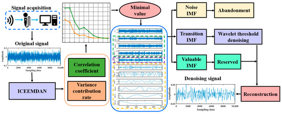
Figure 1.
ICEEMDAN-wavelet threshold denoising process.
3. Signal Denoising Analysis
3.1. Signal Generation
To evaluate the feasibility of the ICEEMDAN-wavelet threshold denoising method, the signals generated by the following functions were denoised [40]:
where is time, the sampling frequency is 500 Hz, and the sampling data are 2500. is a pure signal, and is the Gaussian white noise. The pure signal and adding noise signal are shown in Figure 2.
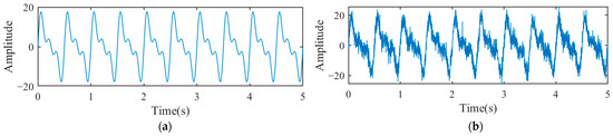
Figure 2.
Signal generation: (a) pure signal; (b) adding noise signal.
As shown in Figure 2b, when Gaussian white noise is added, the smoothness of the pure signal is lost and many burrs appear. In order to separate the pure signal that is drowned by the noise, denoising is required for the noise-added signal.
3.2. Signal Pre-Processing
The noise-added signal is decomposed using the ICEEMDAN method to obtain a series of three-dimensional waveforms of IMFs, as shown in Figure 3a. The spectrum of each IMF component is shown in Figure 3b.
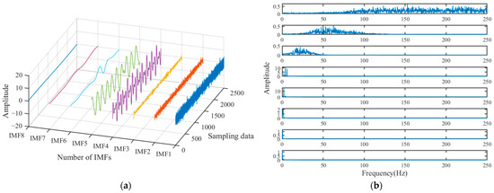
Figure 3.
3D waveform and spectrum of IMF: (a) IMF’s three-dimensional waveforms (Explanation: Blue is the first order IMF, red is the second order IMF, orange is the third order IMF, and so on up to the eighth order IMF.); (b) Spectrum of IMF.
It is observed that IMF1 and IMF2 predominantly consist of high-frequency noise signals, while IMF3 contains both noise signals and valuable signals, classifying it as the transition component. On the other hand, IMF4 and IMF5 are primarily composed of valuable signals. To facilitate a more precise separation of valuable, transition, and noise signals, and to ensure the separation accuracy, the correlation coefficient and variance contribution rate of each IMF component are calculated using Equations (12) and (13). The results are illustrated in Figure 4.
is the IMF and is the IMF mean. is the original signal and is the original signal mean.
is the jth IMF, is the variance of the jth IMF, and is the corresponding variance contribution rate.
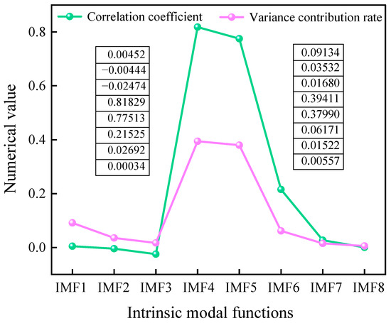
Figure 4.
Correlation coefficient and variance contribution rate of IMF.
The results indicate a consistent correlation coefficient and variance contribution rate, demonstrating the separation accuracy of valuable and noise signals. A minimum occurs at IMF3, where anything less than the minimum point is considered a noise component, and anything greater than the minimum point is considered a valuable signal component. Within valuable signal components, both IMF4 and IMF5 exhibit correlation coefficients exceeding 0.75 and variance contribution rates exceeding 35%, reflecting that they can directly enter the signal reconstruction process. On the other hand, IMF1 and IMF2 demonstrate correlation coefficients close to 0, classifying them as noise components to be discarded. IMF3, identified as a transition signal component, requires denoising via the wavelet threshold to retain more valuable signals.
3.3. Optimization of Wavelet Threshold Parameters
In wavelet threshold denoising, there is no specific criterion for selecting wavelet bases and decomposition layers, and conventional single evaluation indices have limitations in assessing the denoising effect. Various evaluation indices such as the root mean square error, signal-to-noise ratio, smoothness, and correlation coefficient can be used to evaluate the denoising effect from different physical perspectives. In order to denoise signals, this study employs various wavelet basis functions ranging from sym3 to sym8 and performs wavelet decomposition across three to eight layers. Meanwhile, to resolve the shortcomings of the conventional single evaluation index, the root mean square error, smoothness, and correlation coefficient are used as analysis metrics to evaluate the denoising performance, determine the optimal wavelet basis, and optimize the number of decomposition layers. The obtained results are shown in Figure 5.
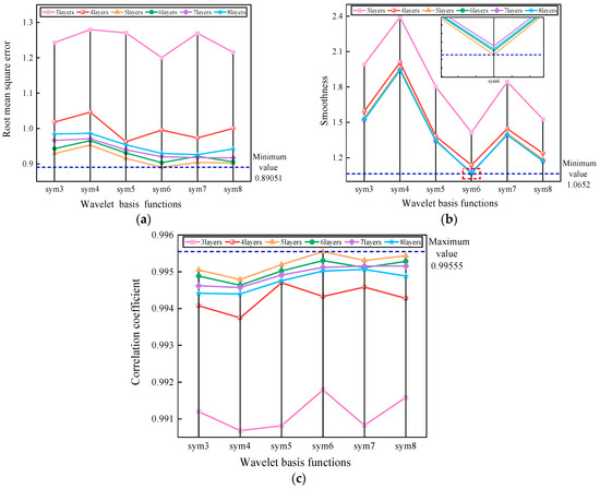
Figure 5.
Calculation results of evaluation indexes: (a) root mean square error; (b) smoothness; and (c) correlation coefficient.
It is worth noting that the root mean square error reflects detailed information and a smaller root mean square error value indicates a more effective denoising process. The smoothness is an index reflecting the overall characteristics of the denoised signal and focuses on the approximation information. A smaller smoothness value corresponds to a superior denoising process. Furthermore, the correlation coefficient reflects the similarity between the denoised and original signals. As a result, the larger the correlation coefficient, the better the denoising effect and the higher the similarity degree in between. Figure 5 reveals that selecting sym6 as the wavelet basis function and employing five decomposition layers results in the lowest root mean square error smoothness values, along with the highest correlation coefficient value. This analysis demonstrates that the transition signal components can be effectively denoised using the wavelet threshold method with the sym6 wavelet basis function and five layers.
3.4. Comparison of Denoising Methods
In order to evaluate the performance of the established denoising method, comparisons were made with three commonly used denoising techniques, including ICEEMDAN, Wavelet threshold, and ICEEMDAN-wavelet threshold denoising methods. In this regard, the root mean square error, smoothness, and correlation coefficient were used as indicators to compare the performance of different methods. The computational results are shown in Table 1. Furthermore, the spectrum of the pure signal and denoised signals are shown in Figure 6.

Table 1.
Calculation of evaluation indicators.
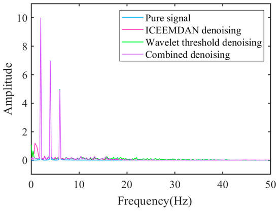
Figure 6.
Spectrum of pure signal and denoised signals.
Table 1 shows that the ICEEMDAN-wavelet threshold combination denoising method yields the lowest root mean square error and smoothness values, as well as the highest correlation coefficient values. Meanwhile, Figure 6 indicates that the high-frequency portion of the spectrum obtained using the combined denoising method is smoother and overlaps with the frequency and amplitude of the pure signal. It is inferred that the combined ICEEMDAN-wavelet threshold denoising performs better than either method alone. The results demonstrate that the ICEEMDAN-wavelet threshold denoising method exhibits an excellent effect in reducing the background noise, thereby establishing a foundation for the subsequent denoising of the collected signals.
4. Experimental Signal Analysis
4.1. Experimental Platform
In order to collect sound signals from the runner blades of a hydraulic turbine during operation, an experimental setup was designed and produced. Experiments were conducted to verify the feasibility of the ICEEMDAN-wavelet threshold denoising method in removing the background noise of the collected signals. The experimental platform is shown in Figure 7 and Figure 8. The experimental platform mainly consists of a water tank, a pressurized pump, a submersible pump, and a hydro generator. At the beginning of the experiment, the water tank is filled with water, and then the pressure pump and submersible pump are turned on simultaneously. The pressure pump pumps water to the hydro generator unit, causing the runner blades to rotate. Meanwhile, the submersible pump pumps the water back into the tank, completing the cycle. When the system reaches a steady-state condition, sediment is added to the water tank and the sound signal caused by the impact of the sediment and runner blades is collected using the sound sensor.
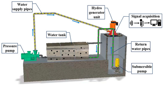
Figure 7.
Three-dimensional view of the experimental platform.
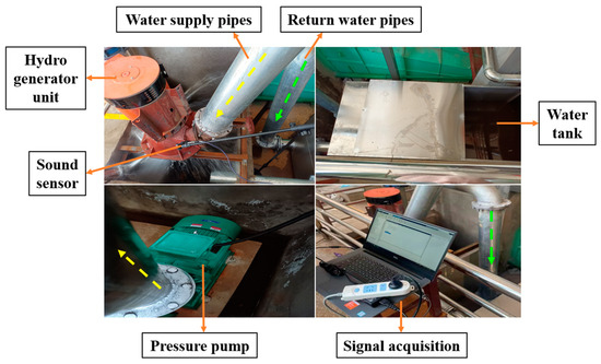
Figure 8.
Experimental platform physical picture.
4.2. Experimental Materials and Equipment
During flood seasons, the sediment content in the river increases dramatically and the water flow carries many large sediment particles. Although the sand sink can filter out a large portion of large sediments, a part of the particles may enter the hydraulic turbine, resulting in severe wear of the runner blades. In order to simulate the sediment water flow during flood seasons, two sediment sizes were used in the experiment: 2–3 mm and 3–4 m (12 kg). To this end, sediment particles were sorted using various sieves with mesh sizes of 2 mm, 3 mm, and 4 mm. The experimental material is shown in Figure 9.
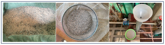
Figure 9.
Experimental material.
The signal acquisition equipment uses an industrial-grade noise sensor, which integrates a microphone, preamplifier, and data acquisition card, with a maximum sampling rate of 48 kHz and a measurement frequency range of 10–20,000 Hz. The noise sensor was fixed near the hydraulic turbine runner using a bracket.
4.3. Signal Denoising
The experiments were conducted and the signals generated by the collision of 2–3 mm and 2–4 mm sediment particles on the runner blades were collected and analyzed. Firstly, the sound signal of a normal operation of the hydraulic turbine with clean water is collected and the results are shown in Figure 10a. It is observed that the signal contains high-frequency noise interference induced by the pressure pump, submersible pump, and hydropower unit operation. In order to facilitate the spectral analysis, the high-frequency background noise should be filtered out. Secondly, the screened 2–3 mm and 3–4 mm sediment were added into the water and the sound signals were collected as shown in Figure 10b,c.
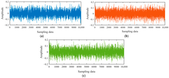
Figure 10.
Original signal of different operating conditions: (a) clean water operating condition; (b) 2–3 mm sediment operating condition; and (c) 2–4 mm sediment operating condition.
The results reveal that the time-domain signals show complex and tight fluctuations with a wide amplitude distribution. The collected signals contain both signals induced by the sediment water flow impacting the hydraulic turbine runner blades and the high-frequency noise signals generated via the operation of pressurized pumps, submersible pumps, and hydropower units. Therefore, the original signals should be initially processed to reduce noise and obtain valuable signals. To accurately separate valuable signals, transition signals, and noise signals, the optimized ICEEMDAN-wavelet threshold denoising method was applied to the original acoustic signals collected under different operating conditions. First, ICEEMDAN is performed on the time-domain signals under the three operating conditions. The first eight orders of IMF are obtained, as shown in Figure 11. The correlation coefficients and the variance contribution rate of the modal components are calculated as shown in Figure 12. With the modal decomposition in Figure 11 and the calculation results in Figure 12, valuable signals, transition signals, and noise signals are filtered out.
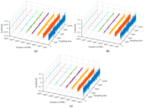
Figure 11.
IMF under different operating conditions (Explanation: Blue is the first order IMF, red is the second order IMF, orange is the third order IMF, and so on up to the eighth order IMF.): (a) IMF under clean water operating condition; (b) IMF under 2–3 mm sediment operating condition; and (c) IMF under 2–4 mm sediment operating condition.
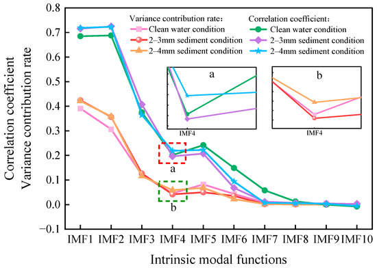
Figure 12.
Correlation coefficient and variance contribution rate of experimental signal.
As shown in Figure 11, the original signals are decomposed into multiple single-component signals containing different waveform components. Combined with the calculation results in Figure 12, IMF4 exhibits the lowest value, indicating that it represents a transition signal component suitable for wavelet threshold denoising. Moreover, the IMF1 to IMF3 components exhibit a tight and complex waveform structure, classifying them as high-frequency background noise, so they are discarded. IMF5 and IMF6 are used as the dominant modal components in the valuable signal components. These components are then reconstructed along the denoised signal to generate the complete denoised signal, as shown in Figure 13.

Figure 13.
Filtered signal of different operating conditions: (a) clean water operating condition; (b) 2–3 mm sediment operating condition; and (c) 2–4 mm sediment operating condition.
4.4. Experimental Signal Characterization
In order to obtain valuable information from the signals, this paper analyzes the filtered signals under different operating conditions in terms of both spectral characteristics and sample entropy characteristics.
4.4.1. Spectral Characteristics
The Fourier transform of the denoised time-domain signal is used to obtain the spectrum, which helps study the frequency distribution characteristics of the sound signal. The spectrum of three different operating conditions is shown in Figure 14.
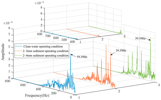
Figure 14.
Spectrum of different operating conditions.
As shown in Figure 14, the high-frequency part of the signal is relatively smooth and the amplitude of the frequency components above 450 Hz tends to zero, indicating that noise caused by pressure pumps, submersible pumps, and hydro generator unit operation can be effectively filtered out. Moreover, there is a standard frequency component of 59.39 Hz in the three operating conditions, indicating that the water flowing through the hydro generator unit produces an inherent frequency.
When operating with clean water, the water flow is relatively stable, so the sound signal mainly contains the vibration frequency of 59.39 Hz induced by the water impacting the runner blades. When water containing 2–3 mm sediment particles passes the turbine, the main frequency component, which is higher than 59.39 Hz, appears. This frequency originates from the collision of sediment particles with the runner blades. Meanwhile, friction and collision occur between sediment particles, generating high-frequency sound signals. Compared with the operating condition with the 2–3 mm sediment, the sound signal of the 2–4 mm sediment contains more high-frequency components. This may be attributed to the higher inertia of the larger sediment particles. The friction and collision between particles enhance the impact on the blades to be more significant, thereby intensifying the high-frequency components of the sound signal.
Based on the above analysis, it is inferred that the sound signal spectrum characteristics are affected by the particle size of sand. More specifically, the sediment water flow produces more high-frequency components than the clean water. Additionally, it is worth noting that as the sediment particle size increases, more high-frequency components appear. Accordingly, the analysis of the spectral characteristics of the sediment water flow can provide a reference for determining whether the hydraulic turbine needs a protective shutdown during the flood season.
4.4.2. Sample Entropy Characteristics
The sample entropy is a characteristic parameter used to describe the complexity of the signal. It is a suitable measure for the analysis of non-smooth nonlinear signals, which are calculated as follows:
- Construct an m-dimensional vector using the data samples {,1 ≤ ≤ N};
- Define the absolute value of the maximum difference between the two corresponding elements of the vector and as the distance , i.e.,
- The number of statistical distances d should not be more significant than the similarity threshold , , for 1 ≤ ≤ , which is defined as;
- Calculate the mean of ;
- Let the dimension be + 1, repeat steps 1 to 4, then calculate and obtain and ;
- Calculate the sample entropy.
Since the sound signals collected in the experiment have non-smooth nonlinear characteristics, the complexity of the acoustic signal should gradually increase when the operating condition of the hydraulic turbine transits from clean water to the 2~4 mm sediment operating conditions. The complexity of the water flow can be evaluated by calculating the sample entropy eigenvalues under different operating conditions. The calculation results are shown in Figure 15.
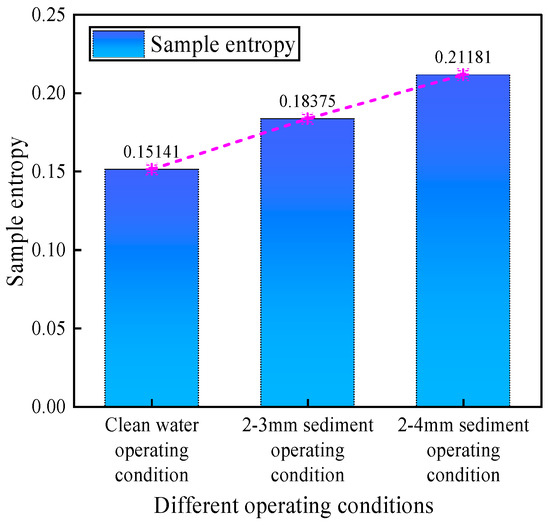
Figure 15.
Sample entropy of different operating conditions.
Figure 15 shows that when the system operates with clean water, the sample entropy value reaches its lowest value. This is because in the absence of sand particles, clean water moves smoothly and the complexity of the sound signal generated when flowing through the hydraulic turbine is low. However, when the flow transitions from the clean water operating condition to the 2–4 mm sediment operating condition, the sample entropy value increases continuously. This is because sediment particles form high-frequency components of the sound signal when impacting the runner blades. As the particle size increases, the inertia of the sediment particles is enhanced. Consequently, the impact on the blades becomes more significant, thereby forming more high-frequency sound components. Meanwhile, these high-frequency components increase the complexity of the sound signal. In summary, evaluating the complexity of the water flow according to the size of the sample entropy is more conducive to analyzing the distribution of sediment particle size in the sediment water flow, thereby avoiding severe abrasion of the hydraulic turbine caused by large-size sediment during the flood season.
5. Conclusions
- (1)
- In this paper, the optimized ICEEMDAN-wavelet threshold denoising method is employed to process the acoustic vibration signals of three operating conditions of the hydraulic turbine. The characteristics of the acoustic signals were analyzed using spectrograms and sample entropy. The results show that when clean water flows through the turbine, the sample entropy reach its smallest values and the dominant frequency component in the spectrogram is 59.39 Hz. When transitioning from clean water to the flood flow containing 2–4 mm sediment particles, the sample entropy is increasing and a high-frequency component higher than 59.39 Hz becomes the prominent frequency of the spectrogram. Meanwhile, the formation of high-frequency components increases with the sediment particle size. Therefore, based on the spectral characteristics and sample entropy characteristics of the sediment water flow, it can provide a reference for whether the hydraulic turbine needs a protective shutdown during flood seasons.
- (2)
- Starting from the acoustic vibration signals of the sediment water flow impacting the hydraulic turbine, the spectral characteristics and sample entropy characteristics of the signals under different operating conditions are analyzed. The results show apparent differences in the characteristics’ noise under different operating conditions, indicating that it is feasible to use the characteristics of acoustic vibration signals to analyze the operating conditions under which the hydraulic turbine is operating. Meanwhile, it can be concluded from the experimental results that the ICEEMDAN-wavelet threshold denoising method is effective in the background noise removal of acoustic vibration signals.
- (3)
- The analysis of acoustic vibration signals of the sediment water flow can provide a supplement for the existing hydraulic turbine condition monitoring system and a new avenue for subsequent research on early warning of hydraulic turbine failure.
Author Contributions
Methodology, software, writing—original draft preparation, and writing—review and editing, S.B.; conceptualization, resources, supervision, and funding acquisition, Y.Z.; writing—review and formal analysis, F.D.; investigation, B.X.; investigation, X.L.; funding acquisition and resources, J.Q. All authors have read and agreed to the published version of the manuscript.
Funding
This research was funded by the National Natural Science Foundation of China, grant number 52079059, and the National Natural Science Foundation of China, grant number 52269020.
Data Availability Statement
Data are requested from the author.
Conflicts of Interest
The authors declare no conflict of interest.
Glossary
| EMD | Empirical modal decomposition |
| EEMD | Ensemble empirical modal decomposition |
| CEEMD | Complete ensemble empirical modal decomposition |
| CEEMDAN | Complete ensemble empirical modal decomposition with adaptive noise |
| ICEEMDAN | Improved complete ensemble empirical modal decomposition with adaptive noise |
| SampEn | Sample entropy |
| The ratio of the signal-to-noise ratio of the added noise relative to the original signal to the standard deviation of the added noise | |
| ( = 1, 2, …, ) | A series of Gaussian white noise with mean 0 and unit variance 1 |
| The th order residual | |
| The th IMF component after EMD | |
| The local mean of the decomposed signal | |
| <> | The mean value for all iterations |
| Original wavelet coefficients | |
| Wavelet coefficients processed by the threshold function | |
| The sign function |
References
- Jakimavičius, D.; Adžgauskas, G.; Šarauskienė, D.; Kriaučiūnienė, J. Climate Change Impact on Hydropower Resources in Gauged and Ungauged Lithuanian River Catchments. Water 2020, 12, 3265. [Google Scholar] [CrossRef]
- Solarin, S.A.; Bello, M.O.; Olabisi, O.E. Toward sustainable electricity generation mix: An econometric analysis of the substitutability of nuclear energy and hydropower for fossil fuels in Canada. Int. J. Green Energy 2021, 18, 834–842. [Google Scholar] [CrossRef]
- Shiji, C.; Dhakal, S.; Ou, C. Greening small hydropower: A brief review. Energy Strategy Rev. 2021, 36, 100676. [Google Scholar] [CrossRef]
- Bocchiola, D.; Manara, M.; Mereu, R. Hydropower Potential of Run of River Schemes in the Himalayas under Climate Change: A Case Study in the Dudh Koshi Basin of Nepal. Water 2020, 12, 2625. [Google Scholar] [CrossRef]
- Šarauskienė, D.; Adžgauskas, G.; Kriaučiūnienė, J.; Jakimavičius, D. Analysis of Hydrologic Regime Changes Caused by Small Hydropower Plants in Lowland Rivers. Water 2021, 13, 1961. [Google Scholar] [CrossRef]
- Paschmann, C.; Vetsch, D.F.; Boes, R.M. Design of Desanding Facilities for Hydropower Schemes Based on Trapping Efficiency. Water 2022, 14, 520. [Google Scholar] [CrossRef]
- Chen, C.; Yang, J.; Liu, Z. Mechanism of Reservoir Bank Deformation and Failure in JinpingⅠ Hydropower Project after Impoundment. Chin. J. Undergr. Space Eng. 2019, 15, 622–628. [Google Scholar]
- Ivarson, M.M.; Trivedi, C.; Vereide, K. Investigations of Rake and Rib Structures in Sand Traps to Prevent Sediment Transport in Hydropower Plants. Energies 2021, 14, 3882. [Google Scholar] [CrossRef]
- Wang, W.; Shang, Y.; Yao, Z. A Predictive Analysis Method of Shafting Vibration for the Hydraulic-Turbine Generator Unit. Water 2022, 14, 2714. [Google Scholar] [CrossRef]
- Jin, Z.; Song, X.; Zhang, A.; Shao, F.; Wang, Z. Prediction for the Influence of Guide Vane Opening on the Radial Clearance Sediment Erosion of Runner in a Francis Turbine. Water 2022, 14, 3268. [Google Scholar] [CrossRef]
- Kumar, D.; Bhingole, P.P. CFD based analysis of combined effect of cavitation and silt erosion on Kaplan turbine. In Proceedings of the 4th International Conference on Materials Processing and Characterzation (ICMPC), Gokaraju Rangaraju Institute Engineering & Technology, Hyderabad, India, 14 March 2015. [Google Scholar]
- Lu, J.L.; Zhang, X.; Wang, W.; Feng, J.J.; Guo, P.C.; Luo, X.Q. Influence of sand particle size on the abrasion performance of hydro-mechanical materials. J. Agric. Eng. 2018, 34, 53–60. [Google Scholar]
- Sharma, S.; Gandhi, B.K. Erosion Wear Behavior of Martensitic Stainless Steel under the Hydro-Abrasive Condition of Hydropower Plants. J. Mater. Eng. Perform. 2020, 29, 7544–7554. [Google Scholar] [CrossRef]
- Rai, A.K.; Kumar, A.; Staubli, T. Analytical modelling and mechanism of hydro-abrasive erosion in pelton buckets. Wear 2019, 436, 203003. [Google Scholar] [CrossRef]
- Tasgin, Y. The Effects of Boron Minerals on the Microstructure and Abrasion Resistance of Babbitt Metal (Sn-Sb-Cu) Used as Coating Materials in Hydroelectric Power Plants. Int. J. Met. 2020, 14, 257–265. [Google Scholar] [CrossRef]
- Singh, R.; Kumar, D.; Mishra, S.K.; Tiwari, S. Laser cladding of Stellite 6 on stainless steel to enhance solid particle erosion and cavitation resistance. Surf. Coat. Technol. 2014, 251, 87–97. [Google Scholar] [CrossRef]
- Kumar, D.; Tu, D.; Zhu, N.; Shah, R.A.; Hou, D.; Zhang, H. The Free-Swimming Device Leakage Detection in Plastic Water-filled Pipes through Tuning the Wavelet Transform to the Underwater Acoustic Signals. Water 2017, 9, 731. [Google Scholar] [CrossRef]
- Wang, L.; Liu, H.; Zhou, L.; Jiang, X.; Li, Y. Numerical Simulation of the Sound Field of a Five-Stage Centrifugal Pump with Different Turbulence Models. Water 2019, 11, 1777. [Google Scholar] [CrossRef]
- Shi, X.; Zhang, Z.; Xia, Z.; Li, B.; Gu, X.; Shi, T. Application of Teager–Kaiser Energy Operator in the Early Fault Diagnosis of Rolling Bearings. Sensors 2022, 22, 6673. [Google Scholar]
- Zheng, J.; Pan, H. Mean-optimized mode decomposition: An improved EMD approach for non-stationary signal processing. ISA Trans. 2020, 106, 392–401. [Google Scholar] [CrossRef] [PubMed]
- Joshuva, A.; Kumar, R.S.; Sivakumar, S.; Deenadayalan, G.; Vishnuvardhan, R. An insight on VMD for diagnosing wind turbine blade faults using C4.5 as feature selection and discriminating through multilayer perceptron. Alex. Eng. J. 2020, 59, 3863–3879. [Google Scholar] [CrossRef]
- Guo, Y.; You, Z.; Wei, B. Working Mode Identification Method for High Arch Dam Discharge Structure Based on Improved Wavelet Threshold—EMD and RDT Algorithm. Water 2022, 14, 3735. [Google Scholar] [CrossRef]
- Xie, X.; Zhang, X. Pre-filtered and post-filtered 1-bit delta sigma modulator for fronthaul downlinks. Opt. Commun. 2022, 510, 127908. [Google Scholar] [CrossRef]
- Zhang, W.; Lv, W.; Hu, A.; Miao, J. A Novel Variational Digital Filtering Method. In Proceedings of the 2022 16th IEEE International Conference on Signal Processing (ICSP), Beijing, China, 21–24 October 2022. [Google Scholar]
- Selesnick, I.W.; Graber, H.L.; Pfeil, D.S.; Barbour, R.L. Simultaneous Low-Pass Filtering and Total Variation Denoising. IEEE Trans. Signal Process. 2014, 62, 1109–1124. [Google Scholar] [CrossRef]
- Zhang, Q.; Lu, G.; Zhang, C.; Xu, Y. Time-frequency analysis of torsional vibration signals based on the improved complete ensemble empirical mode decomposition with adaptive noise, Robust independent component analysis, and Prony’s methods. J. Vib. Control 2022, 28, 3728–3739. [Google Scholar] [CrossRef]
- Li, C.; Peng, T.; Zhu, Y.; Lu, S. Noise reduction method of shearer’s cutting sound signal under strong background noise. Meas. Control 2022, 55, 783–794. [Google Scholar] [CrossRef]
- Ouelaa, Z.; Younes, R.; Djebala, A.; Hamzaoui, N.; Ouelaa, N. Comparative study between objective and subjective methods for identifying the gravity of single and multiple gear defects in case of noisy signals. Appl. Acoust. 2022, 185, 108432. [Google Scholar] [CrossRef]
- Zhang, C.; Fu, S.; Ou, B.; Liu, Z.; Hu, M. Prediction of Dam Deformation Using SSA-LSTM Model Based on Empirical Mode Decomposition Method and Wavelet Threshold Noise Reduction. Water 2022, 14, 3380. [Google Scholar] [CrossRef]
- Fei, H.; Shan, J. Application of CEEMDAN-Wavelet Threshold Method in Blasting Vibration Signal Processing. Blasting 2022, 39, 41. [Google Scholar]
- He, C.; Shi, H.; Si, J.; Li, J. Physics-informed interpretable wavelet weight initialization and balanced dynamic adaptive threshold for intelligent fault diagnosis of rolling bearings. J. Manuf. Syst. 2023, 70, 579–592. [Google Scholar] [CrossRef]
- Pasqualetto, E.; Lunghi, G.; Rocchio, B.; Mariotti, A.; Salvetti, M.V. Experimental characterization of the lateral and near-wake flow for the BARC configuration. Wind Struct. 2022, 34, 101–113. [Google Scholar]
- Buresti, G.; Lombardi, G.; Bellazzini, J. On the analysis of fluctuating velocity signals through methods based on the wavelet and Hilbert transforms. Chaos Solitons Fractals 2004, 20, 149–158. [Google Scholar] [CrossRef]
- Yu, Y.; Li, E.; Yang, P.; Tang, J.; Zhao, X.; Liang, Z.M. Improved TFCA method for AE signal feature extraction of rolling bearing fault. J. Aerosp. Dyn. 2023, 1–10. [Google Scholar] [CrossRef]
- Tian, L. Seismic spectral decomposition using short-time fractional Fourier transform spectrograms. J. Appl. Geophys. 2021, 192, 104400. [Google Scholar] [CrossRef]
- Esmaeilpour, M.; Cardinal, P.; Koerich, A.L. Multidiscriminator Sobolev Defense-GAN Against Adversarial Attacks for End-to-End Speech Systems. IEEE Trans. Inf. Forensics Secur. 2022, 17, 2044–2058. [Google Scholar] [CrossRef]
- Moezi, A.; Kargar, S.M. Simultaneous fault localization and detection of analog circuits using deep learning approach. Comput. Electr. Eng. 2021, 92, 107162. [Google Scholar] [CrossRef]
- Guan, Y.; Tong, P.; Feng, Z. Characterization of planetary gearbox fault current signal based on ICEEMDAN method and frequency demodulation. Vib. Shock. 2019, 38, 41–47. [Google Scholar]
- Qin, G.; Gao, J.; Ye, H.; Jiang, G.; Huang, S.; Lai, X. Tool wear prediction based on fusion of evaluation index and neural network. J. Mil. Eng. 2021, 42, 2013–2023. [Google Scholar]
- Hu, L. Vibration Signal Analysis and Fault Diagnosis of Axial Hydraulic Turbine Generator Set; North China University of Water Conservancy and Hydropower: Zhengzhou, China, 2020. [Google Scholar]
Disclaimer/Publisher’s Note: The statements, opinions and data contained in all publications are solely those of the individual author(s) and contributor(s) and not of MDPI and/or the editor(s). MDPI and/or the editor(s) disclaim responsibility for any injury to people or property resulting from any ideas, methods, instructions or products referred to in the content. |
© 2023 by the authors. Licensee MDPI, Basel, Switzerland. This article is an open access article distributed under the terms and conditions of the Creative Commons Attribution (CC BY) license (https://creativecommons.org/licenses/by/4.0/).