Method for Distinguishing Sargassum and Zostera in the Seto Inland Sea Using Sentinel-2 Data

Abstract

Coastal blue carbon ecosystems are crucial to mitigating global warming. To accurately calculate the blue carbon stock, the existing amount of each species in seaweed and seagrass (SWSG) beds must be estimated to calculate the amount of CO₂ absorbed by each species. However, there exists no efficient and comprehensive method for separating SWSG species. Remote sensing techniques hold promise in addressing this issue. This study used satellite Sentinel-2 data to differentiate and map the areas in which Sargassum and Zostera flourish in the Seto Inland Sea. A two-step approach was proposed to separate these algae. First, the SWSG bed area was estimated using the bottom index method, which has been commonly used for sediment mapping. Consequently, using spectral characteristics obtained from field surveys, the Sargassum and Zostera distinguishing index was developed to efficiently separate Sargassum and Zostera. This algorithm was applied to Sentinel 2 data to create a distribution map of Sargassum and Zostera in the Seto Inland Sea. When the map was compared with SWSG bed maps, obtained using field survey-based methods, it showed high credibility, meaning that the proposed method can be used to repeatedly and easily understand seasonal changes in SWSG types in this area in the future.

1. Introduction

Seaweed and seagrass (collectively referred to as SWSG) beds play a crucial role in the proliferation of aquatic resources owing to their functioning as spawning grounds for aquatic organisms, such as young and larval fish. Moreover, recently, marine forests have received renewed attention as sites of blue carbon, which absorbs inorganic carbon from water and supplies oxygen [1,2,3,4]. However, in the Seto Inland Sea, which is the study area, regulations on the discharge of nutrients and other salts have been implemented for many years to reduce the eutrophic state represented by red tide [5], which became a problem in the 1960s and 1970s. Consequently, water quality has improved considerably, except in certain areas; however, there have been problems, such as sluggish fish catches and discolored SWSG bets, owing to oligotrophication [6]. Under these circumstances, the “Act on Special Measures concerning Conservation of the Environment of the Seto Inland Sea” [7], which was amended and enforced in April 2022, aims to eliminate the lack of nutrients in the sea and promote “blue carbon”. First, the current status of SWSG bed distribution throughout the year must be understood accurately to achieve this goal. However, the Seto Inland Sea has a complex topography, containing 600 islands at an average depth of 30 m [8]. Furthermore, it exhibits large regional and seasonal tidal differences (approximately 1–3 m and 3–4 m in the eastern and western sea areas, respectively). Conducting quick field surveys over a wide area is difficult and incurs enormous financial costs. The Ministry of the Environment, Government of Japan (MOEJ), compiles the date of field surveys that are reconducted once every few years and publishes a SWSG beds distribution map on the Internet. However, the seasonal changes over a wide area cannot be determined. Therefore, satellite remote sensing technology that can repeatedly grasp the distribution of SWSG beds over a wide area is considered promising for providing accurate estimates of blue carbon. The difficulty in understanding the distribution of SWSG beds using satellite remote sensing is that the influence of light attenuation caused by water is extremely large when determining the presence of SWSG compared to that of the land cover classification on land. Additionally, as the attenuation rate of light underwater is greater for long wavelengths, above-water and information at wavelengths longer than that of near-infrared regions cannot be used and almost only information from light in the visible range can be used. Furthermore, because different types of SWSG often exhibit similar colors, distinguishing species based on their spectral characteristics is challenging. However, these weaknesses have been overcome and SWSG bed distribution maps are now being created using several satellite remote sensing-based several methods.

There are broadly two types of methods for extracting SWSG beds using remote sensing. To extract SWSG, one method involves using existing water depth data, performing water depth correction, and then applying terrestrial land cover classification methods, such as unsupervised or supervised classification, LAI (leaf area index), which can measure leaf area based on optical assumptions regarding light attenuation, and NDVI (Normalized Vegetation Index), which measures plant activity based on red absorption and near-infrared scattering from the leaf, and so on [9,10]. The other method eliminates the influence of water depth and extracts SWSG only from image calculations without using water depth data [11,12]. The former method requires accurate water depth data that considers tidal level changes on the day the satellite image is captured. However, obtaining detailed water depth data in shallow waters is difficult. Thus, water depth estimation using images is often attempted [13,14]. However, this method exhibits poor accuracy in estimating water depth, particularly under conditions of a water depth of 4–5 m or greater. Moreover, it results in excessive water depth correction [unpublished]. The latter method is convenient because it facilitates the extraction of SWSG from satellite images without water depth data. However, it is generally difficult to identify SWSG species because it uses minute differences in the log reflectance ratio of the bottom sediment. Therefore, the latter method is used to extract the SWSG bed area in sea areas, such as the Seto Inland Sea, wherein fairly accurate water depth and water level data can be obtained. In addition, in shallow sea areas of 10 m or less, the water depth data are corrected to determine the spectroscopic SWSG area. A hybrid method that performs species discrimination is considered to be effective. Currently, the MOEJ creates a marine forest map along the coast of Japan using field surveys and high-resolution satellite data, and the maps are classified into Sargassum bed, Zostera bed, and kelp bed [15]. There are also studies focused on the optical detection of Sargassum and Zostera. Gower initially identified Sargassum using the MERIS Maximum Chlorophyll Index [16]. Hu utilized the Floating Algae Index (FAI) with MODIS image data to detect Sargassum [17]. Gower and King employed the red-edge concept for Sargassum detection, acknowledging that other marine organisms can also cause elevated red-edge reflectance [18]. Taking into account the characteristic absorption feature of Sargassum at 630 nm, distinct from other floating vegetation, Dierssen et al. developed the Sargassum Index (SI), which uses the bands of 650 and 630 nm [19]. Field measurements by Hu indicated that Sargassum exhibits a distinctive reflectance curvature around 630 nm due to its chlorophyll c pigments [19]. While these methods have effectively diagnosed Sargassum slicks using pre-determined thresholds, a method for distinguishing between Sargassum and Zostera in the Seto Inland Sea using Sentinel-2 data has not been proposed. Yoshida’s study on Sargassum and Zostera in the Seto Inland Sea reveals that Zostera thrives in shallow sandy areas, while Sargassum prefers deeper, rocky, and intertidal zones. In the Seto Inland Sea, Sargassum is mainly composed of three species: S. condusum, S. yezoense, and S. trichophyllum, each with distinct maturity periods ranging from March to June, June to August, and October to December, respectively [20].

Against this background, this study developed and verified a method able to spectroscopically distinguish Sargassum and Zostera in the sea using Sentinel-2 data, which exhibit the highest spatial resolution among currently available free data. This study aimed to understand changes in the distribution over time. To achieve this goal, we first considered detecting marine forests from Sentinel-2 data using a method that did not require water depth data. Subsequently, we proposed a method to separate Sargassum and Zostera based on their spectral reflectance measured in the field. Finally, the distributions of Sargassum and Zostera mapped using this method were integrated and verified through comparisons with existing marine forest maps. If such a method is valid, it will be possible to repeatedly update existing marine forest maps using satellites.

2. Materials and Methods

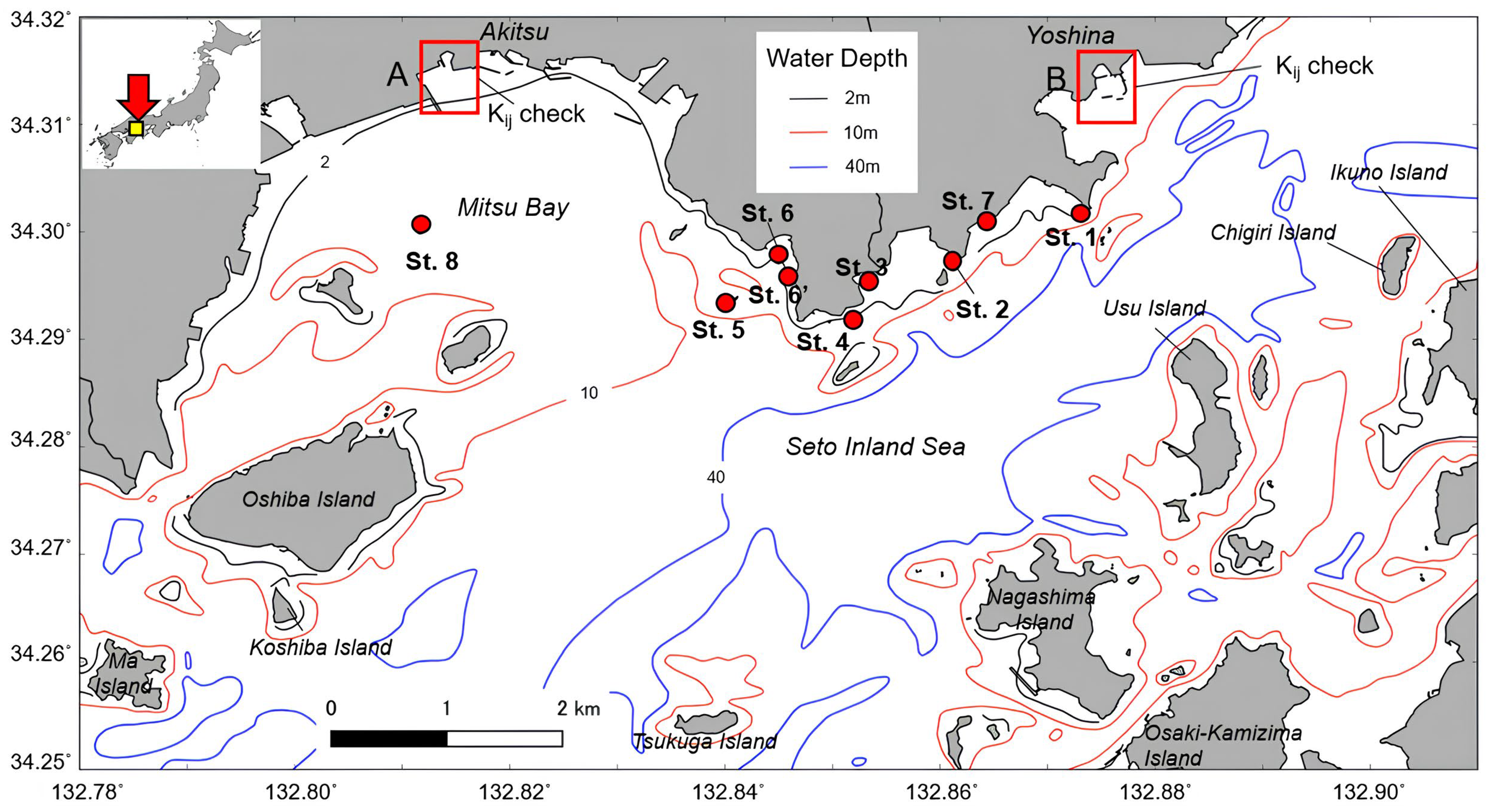
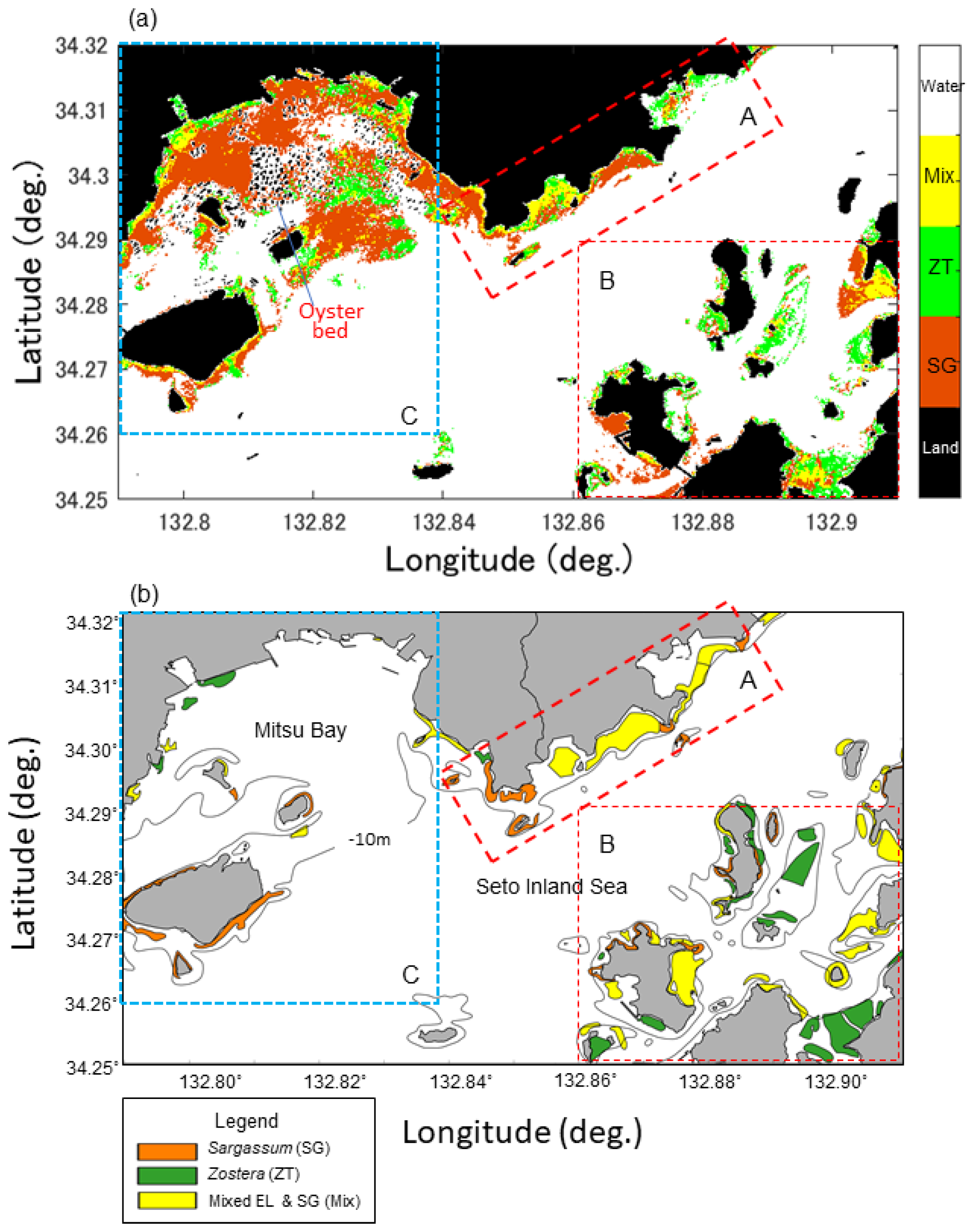
2.1. Study Area

The study area was the Seto Inland Sea off the coast of Takehara City, located in the south-central part of Hiroshima Prefecture, as shown in Figure 1. According to Yoshida et al. [21], the SWSG beds area of the “Bingo–Geiyo–Seto” fishery area (conducted from 1989 to 1991) is 3636 ha. The total areas of seagrass, SWSG, and kelp beds are 2917 ha (80%), 1289 ha (35%), and 184 ha (5%), respectively (as there is mixed marine forest, the total does not add up to 100%). Thus, the Sargassum and Zostera beds are the main SWSG beds in the central Seto Inland Sea. In addition, as for their habitat, Zostera beds are formed in calm sandy mud areas with little wind and waves, whereas Sargassum (formed by brown SWSG Sargassum) is formed in rocky reef areas. In the Seto Inland Sea, there are many areas of water wherein sand and mud and rocky reef areas exist alternately; thus, Sargassum and Zostera beds coexist. These statistics are data for shallow waters below 10 m in depth, and as the marine forest in Figure 1 also exists mostly in shallow waters below 10 m, this study targeted waters below 10 m. In addition, the tidal level difference in the target water area is approximately 4 m at maximum.

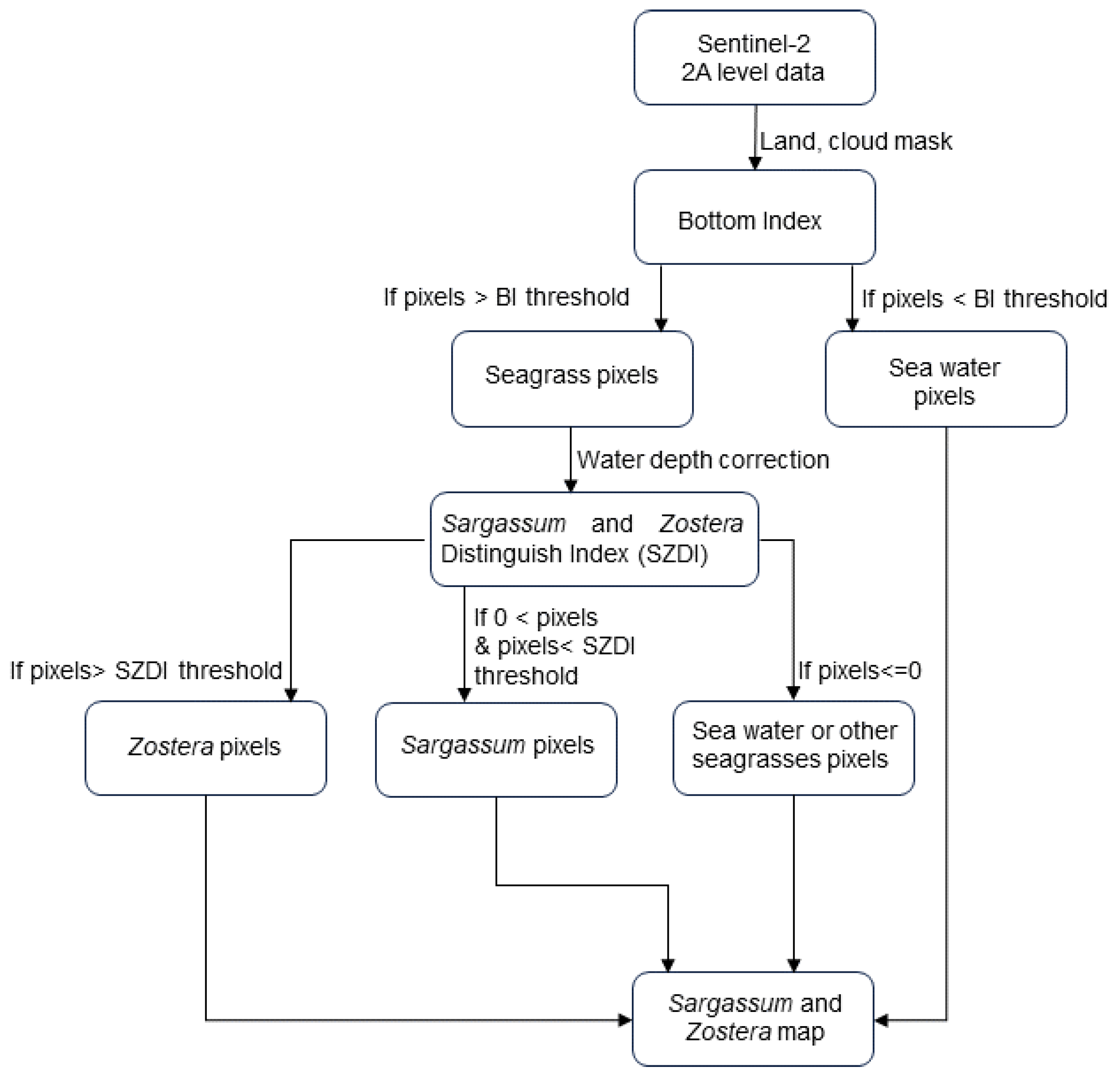
2.2. Separation Method of Sargassum and Zostera Using Satellite Data

Figure 2 shows the procedure for creating a marine forest distribution map used in this study. To briefly explain the overall procedure, first, the acquired satellite data were processed as a land mask using near-infrared threshold processing and a cloud mask using Quality flag data. After correcting the water depth, the SWSG bed area was extracted. Furthermore, the Sargassum and Zostera Distinguishing Index (SZDI) method was proposed and applied to the extracted seagrass beds to separate them into Zostera and Sargassum beds. The most important water depth correction in this process is explained later. The specific method of SZDI is discussed later based on the results of the study.

In general, in underwater analysis, the influence of water dissipation is considerably greater than in land analysis; thus, in waters with a complex seafloor topography (the Seto Inland Sea), stable SWSG beds cannot be extracted without depth correction. Therefore, in remote sensing, there exist two methods: one involves using existing seafloor topography data, converting the underwater reflectance to be equivalent to the reflectance on land, and then performing analysis. The other method utilizes the surface reflectance ratio of two different bands to eliminate the influence of water depth and distinguish between various bottom sediments. Studies have attempted to remove the influence of water depth and extract the bottom sediment (in this case, SWSG beds). This method is referred to as the bottom index (BI) or depth invariant index (DII) [11,12].

First, we explain the former method, which uses seafloor topography data. If seafloor topography data exist, the most basic relationship between the reflectance R immediately above the water surface (equivalent to the atmospherically corrected reflectance of the satellite) and the seafloor reflectance information can be theoretically obtained by using the following formula [22]:

$$R_i=R_{\infty i}\left[1-\exp \left(-{2k}_i{z}_B\right)\right]+R_{Bi}\exp \left(-{2k}_i{z}_B\right),$$

(1)

where R_∞ is the reflectance at an infinite water depth, k is the extinction coefficient of the target seawater, R_B is the underwater extinction coefficient of the band, Z_B is the seafloor depth, and the subscript i is the band. Furthermore, the first term on the right-hand side of Equation (1) accepts an extremely small value compared to the second term on the right-hand side. Therefore, R_B at a water depth of 0 m (equivalent to ground level) can be calculated approximately using the following formula. Hereinafter, such a correction is referred to as “water depth correction”.

$$R_{Bi}\fallingdotseq \frac{R_i}{\exp \left(-{2k}_i{z}_B\right)}.$$

(2)

However, Z_B and k on the day of satellite observation must be known when using this formula. There exists a method to calculate k from the relation between Z_B and the brightness value of the image (the slope when approximated by a logarithmic function); however, if Z_B exceeds several meters, it results in overcorrection. It is extremely difficult to correct the water depth even when targeting topography below 10 m (as in this case). Therefore, we assumed that the extinction coefficients for the three periods were constant. Moreover, a correction coefficient m was introduced to prevent the value of each band from falling below 0, and corrections were made for the three periods using the following formula:

$$R_{Bi}\fallingdotseq \frac{R_i}{\exp \left(-{2m_{i}k}_{s{w}_i}ZB\right)},$$

(3)

where k_sw is the general extinction coefficient of seawater.

Next, we explain the latter method, which does not use bathymetric data. The BI method is based on the theory proposed by Lyzenga [11,12]. The bottom sediment index is a model developed based on the assumption that “if the bottom sediment is the same, the bottom sediment reflectance ratio (natural logarithm type) of two different bands will be constant”. A brief explanation of the theory of sediment indicators is given below. Lyzenga expressed the radiance (L_sλ) detected by a sensor mounted on a satellite in shallow water at wavelength λ using the following formula:

$$L_{s\lambda }=L_{B\lambda }-E_{\lambda }{R}_{B\lambda }\exp \left(-{2k}_{\lambda }{z}_B\right),$$

(4)

where L_Bλ is the radiance observed at a deep point in the water, E_λ is the solar irradiance reaching the ground, R_Bλ is the spectral reflectance of the bottom sediment, k_λ is the spectral extinction coefficient of water, and Z_B is the water depth. Equation (4) is extended to two wavelengths and the effect of water depth is removed by calculating the ratio. Therefore, the radiance observed by the satellite in two different bands i and j is expressed by the following equations using Equation (4).

$$L_{si}=L_{Bi}-E_i{rR}_{Bi}\mathrm{e}\mathrm{x}\mathrm{p}(-{2k}_i{z}_B)$$

(5)

$$L_{sj}=L_{Bj}-E_j{R}_{Bj}\exp \left(-{2k}_j{z}_B\right).$$

(6)

Rearranging Equations (5) and (6), we obtain the following equation with water depth z removed:

$$LN\left[\frac{R_{Bi}{E}_i}{{\left(R_{Bj}{E}_j\right)}^{kij}}\right]=LN\left[\frac{(L_i-L_{si})}{{(L_j-L_{ji})}^{kij}}\right],$$

(7)

where most of the fluctuations on the left side are controlled by the “ratio of seafloor reflectance between the two bands” and contain information related to the bottom sediment. Therefore, this is defined as the BI and is set as the portion on the right side. Consequently, the bottom sediment index can be calculated using the following formula:

$${BI}_{ij}=LN\left[\frac{(L_i-L_{si})}{{(L_j-L_{ji})}^{kij}}\right]=LN\left(L_i-L_{si}\right)-k_{ij}LN\left(L_j-L_{sj}\right).$$

(8)

Using Equation (8), the extinction coefficient ratio k_ij can be defined as the band ratio (the slope when the logarithm of the brightness values of the different bands is plotted) from the relation between the satellite data of two different bands. Theoretically, the influence of water depth can be calculated from the image alone. Consequently, the sediment (in this case, SWSG beds), from which the 200 nm has been removed (in the case of sediments with different reflectance ratios), can be distinguished. The actual extinction coefficient ratio k_ij is calculated at locations with the same bottom material but at different water depths (often using several pixels offshore from a sandy beach). If the slope is derived from the scattering value of the logarithm of the luminance ratio of the two wavelengths (L_s corrected), it is equivalent to the theoretical extinction coefficient ratio. We assumed that the bottom sediment in areas A and B in Figure 1 (estuary area outlined in red) was sand, and four points at different water depths were selected. Equation (8) is at times used as an alternative to reflectance, as shown in the following equation [23]. Equation (9) was adopted herein as well.

$${BI}_{ij}=LN\left(R_i-R_{si}\right)-k_{ij}LN\left(R_j-R_{sj}\right).$$

(9)

2.3. Field Spectral Reflectance Data Sampling

To develop an algorithm to separate Sargassum and Zostera, we primarily used an Ekman–Birge grab sampler and a boat hook to pull Sargassum or Zostera from the seabed onto the ship and measured their spectral reflectance. Figure 3 shows photographs of the Sargassum and Zostera captured underwater before being pulled up (bottom) and on board the ship (top). These were obtained at St. 2 on 19 March 2021 and 17 June 2021, respectively. The reflectance of SWSG was measured using a visible/near-infrared spectroradiometer “MS720” manufactured by EKO Ltd., Bedfordshire, UK (wavelength range: 350–1050 nm, wavelength interval: 3.3 nm) and a device manufactured by Japan Color Research Institute, Saitama, Japan. It is a standard white board (ZB6010). Specifically, the reflectance was calculated by measuring the spectral irradiance of the SWSG and the spectral irradiance of the sunlight reflected by the white board three times from a height of approximately 20 cm directly above the surface and dividing the average value. Furthermore, by gathering SWSG of the same species as close together as possible, the effects of reflection from the background board were reduced. The resulting field survey dates were 19 March, 17 June, 19 July, and 21 September 2021, and the fundamental measurement points were St. 1, St. 2, St. 3 St. 4, St. 5, St. 6, St. 6’, St. 7, and St. 8. However, St. 8, where the measured water depth exceeded 10 m and no SWSG could be confirmed, was not used in the analysis.

2.4. Satellite Data Used and Preprocessing Method

The satellite data used in this study were atmospherically corrected reflectance (level 2) data from the Sentinel-2 multispectral instrument (MSI), which can be downloaded free of charge from the Copernicus Open Access Hub. As shown in

Table 1. Characteristics of Sentinel-2 bands (https://custom-scripts.sentinel-hub.com/custom-scripts/sentinel-2/bands/, accessed on 9 November 2023).

Band	Central Wavelength	Spatial Resolution	Band	Central Wavelength	Spatial Resolution
Band 1	443 nm	60 m	Band 8	842 nm	10 m
Band 2	493 nm	10 m	Band 8a	865 nm	20 m
Band 3	560 nm	10 m	Band 9	945 nm	60 m
Band 4	665 nm	10 m	Band 10	1375 nm	60 m
Band 5	704 nm	20 m	Band 11	1610 nm	20 m
Band 6	740 nm	20 m	Band 12	2190 nm	20 m
Band 7	783 nm	20 m

, MSI originally had 12 bands; however, in this study, data with a higher resolution were desired. Thus, only Band 2 (493 nm), Band 3 (560 nm), and Band 4 (665 nm) with a 10 m resolution were used. The satellite data used were that of 19 March, 23 May, and 27 July, which were close to the on-site observation dates in 2021, as shown in

Table 2. Satellite data used with tidal level.

No.	Sentinel-2 (S-2)				Tidal Level * (m)
	Date	Time	Tile Number	Platform
1	19 March 2021	10:47JST	T53SKU	Sentinel-2B	2.37
2	23 May 2021	10:47JST	T53SKU	Sentinel-2A	0.71
3	27 July 2021	10:47JST	T54SKU	Sentinel-2B	3.19

Note: * Takehara station of Japan Meteorological Agency at 11 am.

. The tide levels for satellite data acquisition were 2.37, 0.71, and 3.19 m, respectively. The k_sw employed for water depth correction using Equation (3) for the preprocessing of satellite images was the actual value of Moreland Prieur [24] (if there was no value for the Sentinel-2 wavelength, the values for the previous and subsequent wavelengths were linearly interpolated); m was used at a water depth of 14 m, which is the maximum water depth to be corrected at 10 m, and the maximum tide level of this area was 4 m. Further, the limit value at which the reflectance of each band did not exceed 1 was used.

Table 3. Water depth correction parameters of Equation.

Sentinel-2 Band	Wavelength (nm)	ksw (m−1)	m
2	493	0.0238	1.37
3	560	0.0720	0.45
4	665	0.4200	0.07

shows the values of k_sw and m of the water depth correction parameters used in this study. Furthermore, Rs in Equation (9) is the reflectance (equivalent to aerosol) in a clean body of water (the open ocean); however, in this case, the open ocean area was not near the target water area. Thus, the minimum value of each band in the screen was set [25] (

Table 4. R_s values on 19 March, 23 May and 27 July 2021.

Date	Rs_Band2	Rs_Band3	Rs_Band4
19 March 2021	0.018	0.165	0008
23 May 2021	0.030	0.050	0.040
27 July 2021	0.020	0.020	0.010

).

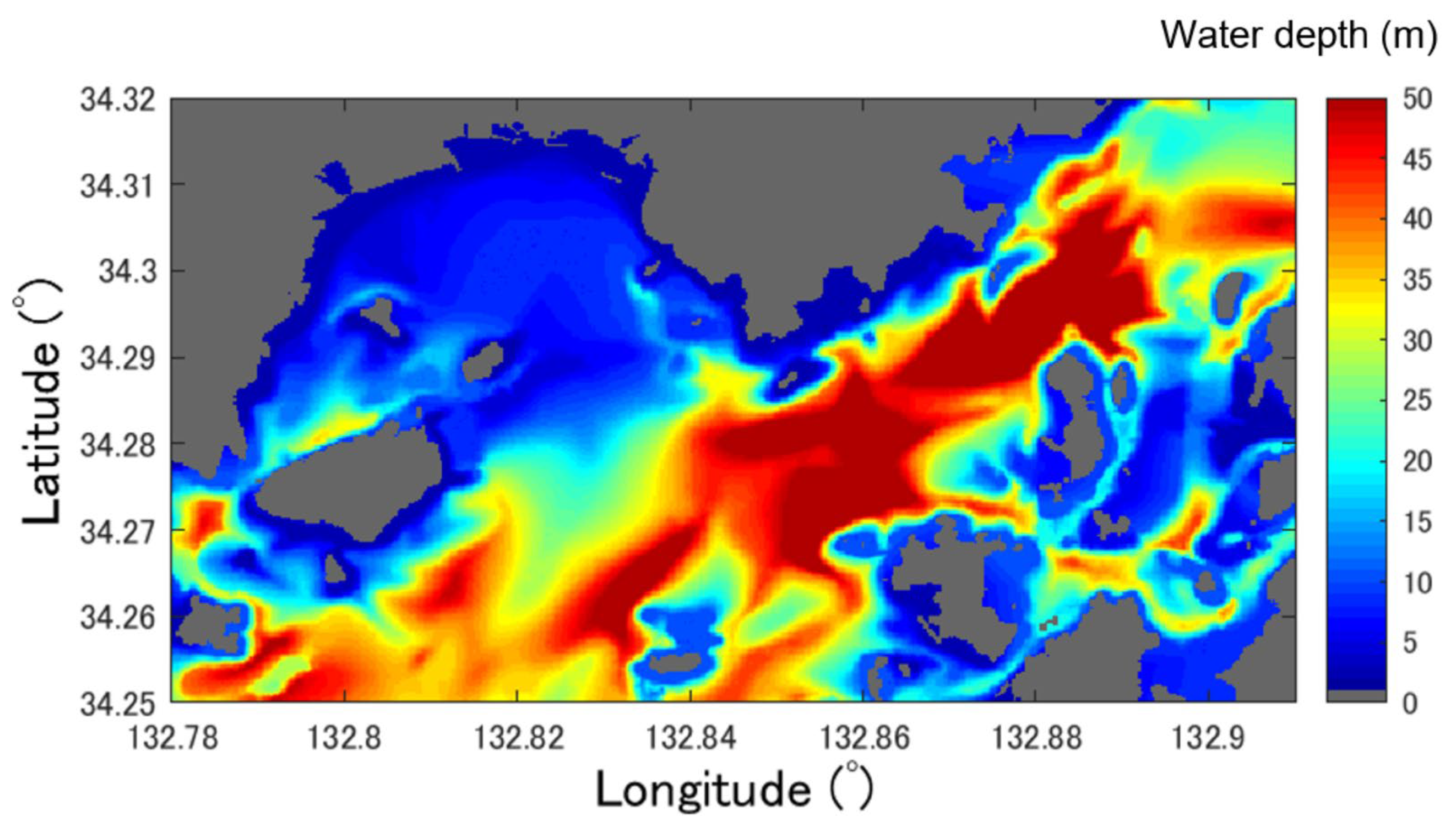
2.5. Digital Water Depth Data

In this study, existing digital water depth data (water depth equivalent to the lowest tide level) were used for water depth correction. Here, the M7000 series, a high-resolution submarine topography dataset along the coast of Japan created by the Japan Hydrographic Association, was employed in the M7018 region of the western Seto Inland Sea. The spacing of the contour lines of M7000 differs depending on the sea area; however, at depths below 100 m, the contour lines are densely spaced at intervals of 1–2 m. We used this irregular point cloud data by resampling it into 10 m mesh data, which is the same as Sentinel-2 data. The bathymetric map obtained in this manner is shown in Figure 4. In addition, when correcting the water depth using Equation (3), these tide levels were added to the water depth data described later.

3. Result

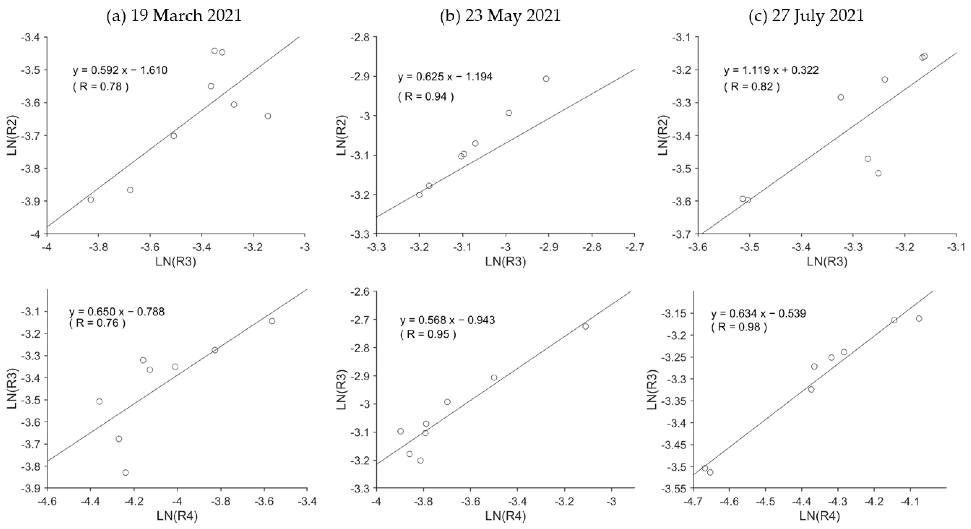
3.1. Extraction Coefficient of Study Area

Equation (9) was used to extract the Sargassum and Zostera areas. First, to determine the extinction coefficient (k_ij) of Equation (7) for the three target periods, we calculated Sentinel-2 Band 2–3 (k23) and Band 3–4 (k23) in the two estuary areas, as shown in Figure 1. The relation (k34) was confirmed (Figure 5). Generally, if the bottom material is the same (here assumed to be sandy soil), a high correlation coefficient should be obtained for the natural logarithm relation between the two. Here, to aim for automation in the future, combinations that have a high correlation coefficient for any date must be selected. Consequently, as shown in Figure 5, all data exhibited almost the same correlation coefficient; however, overall, the correlation coefficient of k34 was higher than that of k23. Thus, k34 was adopted. The Rs in Equation (9) was set as the value shown in Table 3. Figure 6 shows the results of calculating BI by applying this k34 to Equation (9) ((a–c) on the left) and the threshold value that results in a water body with a water depth of approximately 10 m or less. The SWSG beds distribution map obtained when setting (March: −1, May: −0.95, July: −0.60) is shown in red. Hereinafter, this study assumed that this red area was a SWSG bed containing only Sargassum and Zostera.

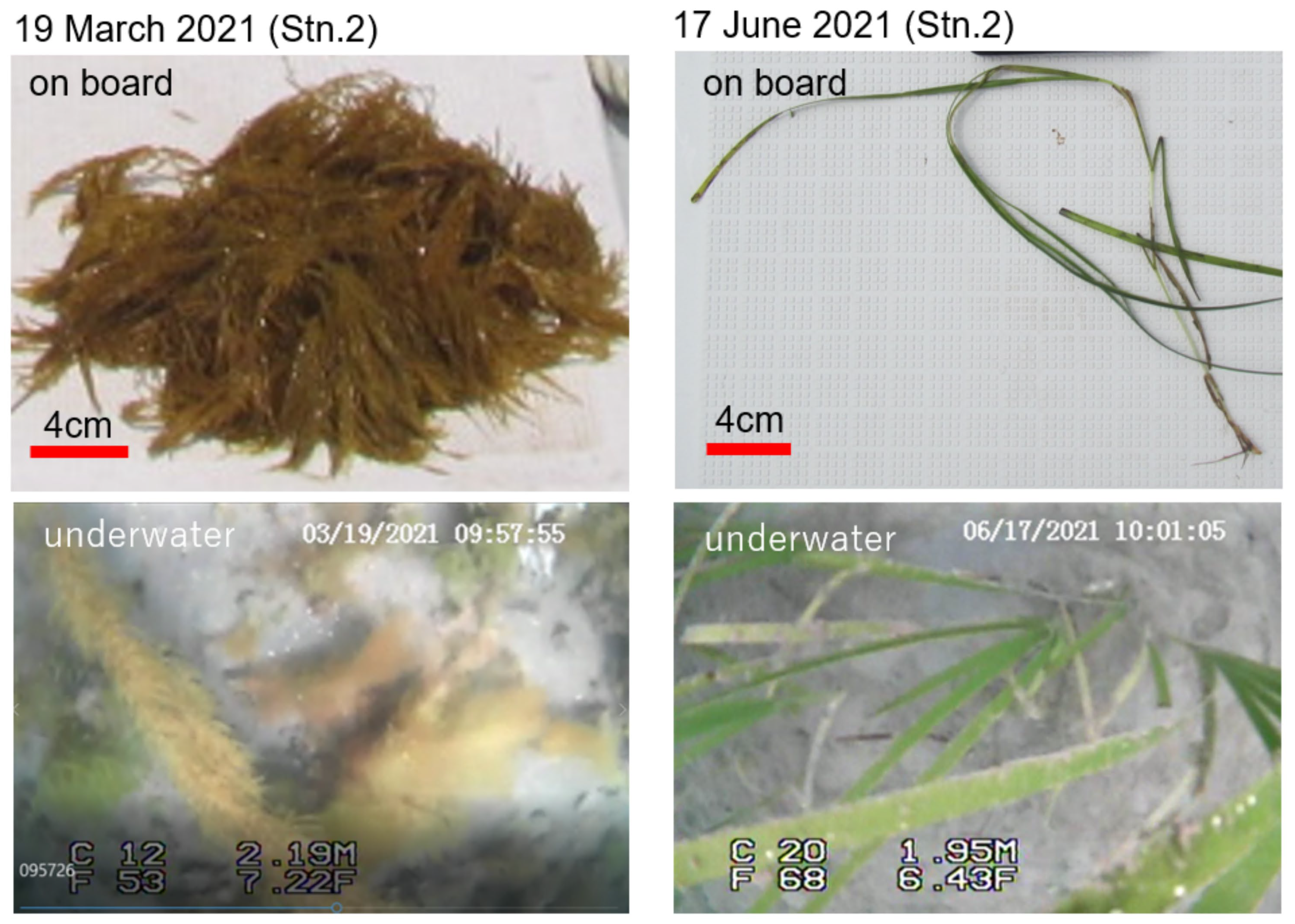
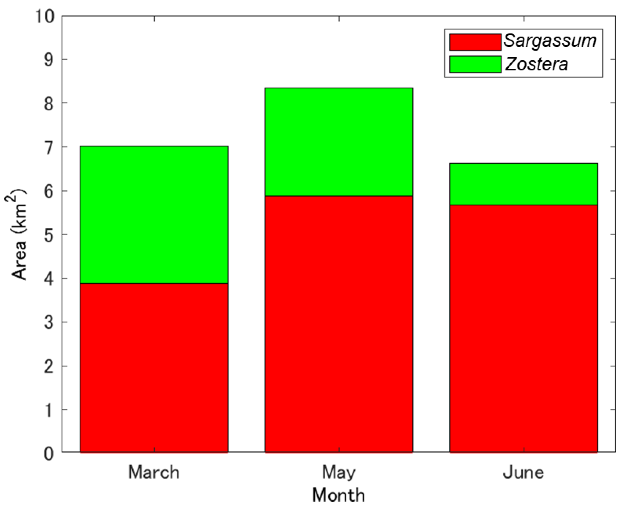
3.2. Overview of Sargassum and Zostera Appearance

An occurrence table of SWSG types was created based on the observation results obtained at St. 1–St. 7 on 19 March, 17 June, 19 July, and 21 September 2021 (

Table 5. Seagrass species observed at each location. “Other” indicates the SWSG beds other than Sargassum and Zostera. “Unknown” indicates a station wherein no survey was conducted on the day, and “None” indicates the absence of SWSG beds.

Date	Stations
	St. 1	St. 2	St. 3	St. 4	St. 5	St. 6	St. 7
19 March	Sargassum	Other	Other	Sargassum	Sargassum	Sargassum	Unknown
17 June	None	Zostera	Zostera	Zostera	Sargassum	None	Zostera
19 July	Zostera	Unknown	Unknown	Other	Sargassum	Unknown	Unknown
21 September	None	None	None	None	None	None	None

). In this table, “other” indicates the SWSG beds other than Sargassum and Zostera, “unknown” indicates a station wherein no survey was conducted on the day, and “none” indicates the absence of SWSG beds. In March 2021, Sargassum appeared at all four stations (St. 1, St. 4, St. 5). In June of the same year, Zostera appeared at all four stations (St. 2, St. 3, St. 4, St. 7) except St. 5, whereas Sargassum only appeared at St. 5. Furthermore, in July, Zostera newly appeared in St. 1. However, no SWSG beds were observed at any of the survey points in September. These facts suggest that the SWSG beds in this region changed seasonally, even at the same station.

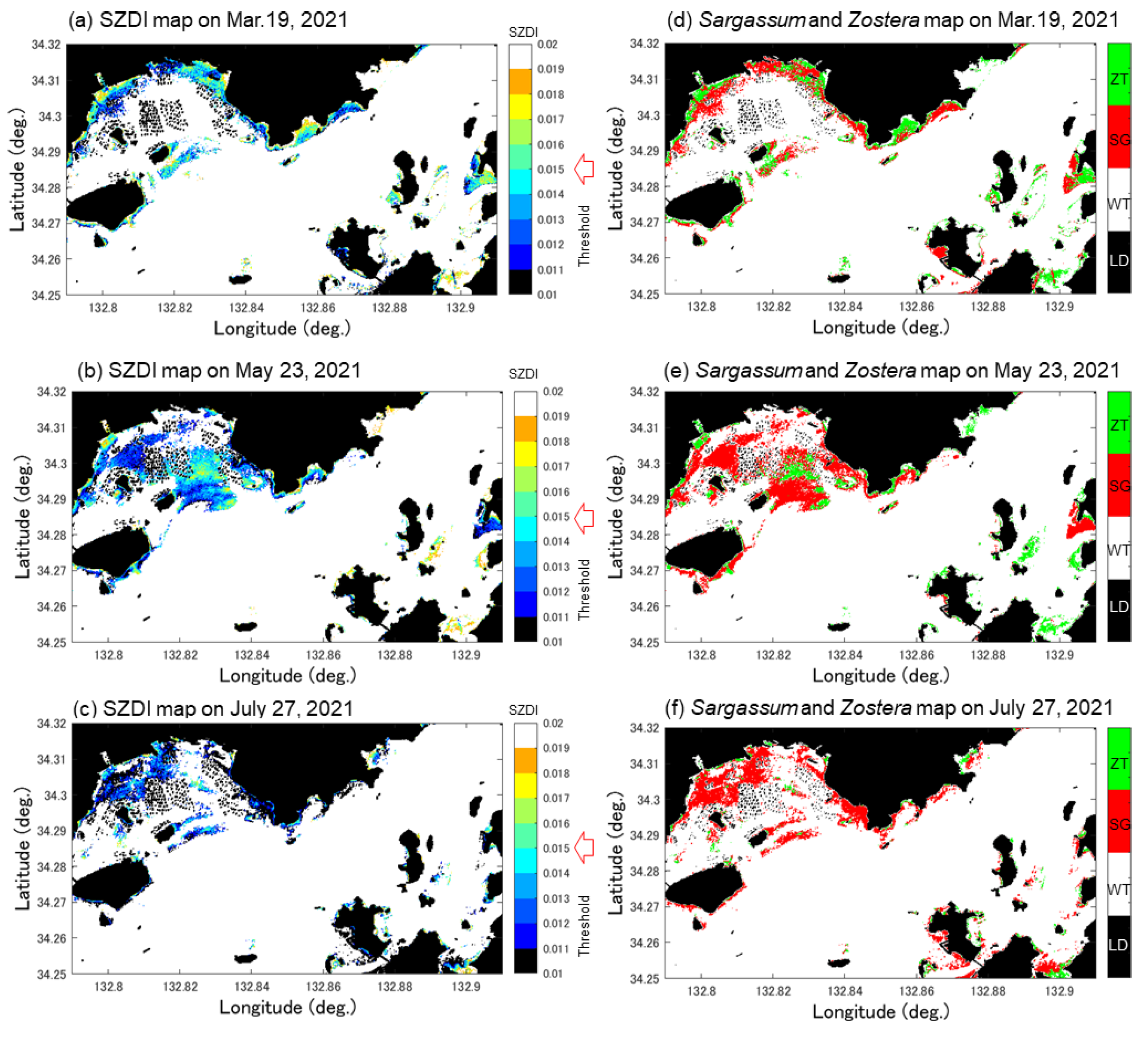
3.3. Proposal of a Method Distinguishing between Sargassum and Zostera

Figure 7a shows the spectral reflectance characteristics of Sargassum and Zostera measured in 2021. The Sargassum at St. 4 and St. 6 on 19 March, as shown in Table 5, was confirmed in the underwater video. However, spectral reflectance data could not be obtained as sampling was not possible. The common spectral characteristics of Sargassum and Zostera are that they both exhibit relatively low reflectance in the 400–500 nm range, relatively high reflectance at approximately 560 nm, and extremely strong absorption above 670 nm. The difference in the peak reflectance between the two was noticeable in the wavelength range of 500–670 nm. Thus, Sargassum and Zostera exhibit different reflectance maxima in the red region at ~600–670 nm (particularly ~610–650 nm) and the green region at 550–570 nm (particularly at ~560 nm). Figure 7b shows a diagram simulating the reflectance characteristics of the wavelengths observed by Sentinel-2. Only at the wavelength observed by Sentinel-2 was the difference in the reflectance between Sargassum and Zostera remarkable. The peak shift in the green and red areas was somewhat unclear in the low reflectance region (in particular, at the red of Sargassum, the peak disappeared).

Figure 8 shows the difference in spectral reflectance when the water depth is changed using Equation (3) for the data with the highest spectral reflectance for Sargassum and Zostera. As evident, the change in reflectance at 493 nm between Sargassum and Zostera was minimal. Moreover, even for red objects, such as Sargassum, the reflection was considerably weakened below a 1 m depth. Furthermore, the red reflectance was ~0 at a ~4-m depth and remained constant at approximately 0 at deeper water depths. However, the green band of Zostera tended to exhibit a considerably higher reflectance than that of Sargassum, at least at depths of ≥5 m.

Based on the above results, Sentinel-2 can distinguish Sargassum and Zostera by changing the green area (560 nm: Sentinel-2 Band 2) reflectance at a depth of approximately 5 m or less, regardless of the water depth. In addition, the relative size of the green band is one indicator. Furthermore, following the floating algae index (FAI) [17,26], which is used to detect floating algae, the background can be detected by obtaining the difference between the line drawn by the reflectance of 493 and 665 nm (baseline) and the green reflectance. It is considered that the contrast between the reflectance of water and SWSG beds would become clearer. Therefore, we defined the SZDI from the relationship shown in Figure 9 and proposed the following calculation formula:

$$SZDI=R_{Green}-R_{Blue}-{R^{\prime }}_{Green}$$

(10)

$${R\prime }_{Green}=\frac{{\lambda }_{Green}-{\lambda }_{Blue}}{{\lambda }_{Red}-{\lambda }_{Blue}}\left(R_{Red}-R_{Blue}\right),$$

(11)

where R is the reflectance, λ is the wavelength, and the subscripts Blue, Green, and Red indicate blue, green, and red bands, respectively (in the case of Sentinel-2, they are 493, 560, and 655 nm, respectively). Hence, when Equations (10) and (11) are applied to satellite data, such as Sentinel-2, the larger the SZDI, the higher the possibility of Sargassum; meanwhile, the smaller the SZDI, the higher the possibility of Zostera.

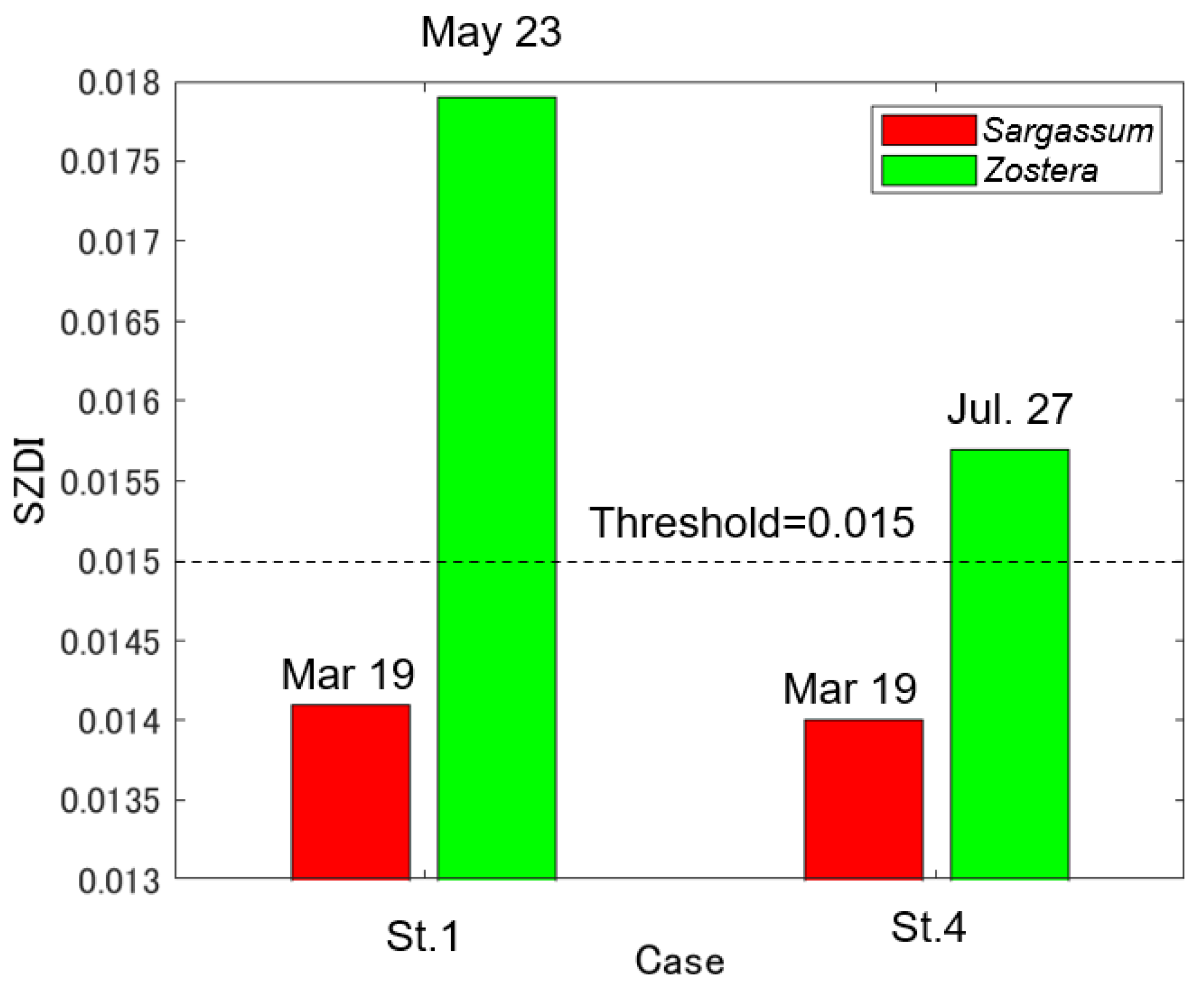
3.4. Validation of the Sargassum and Zostera Distinguish Index

Figure 10 shows the SZDI maps for 19 March, 23 May, and 27 June 2021 (a–c) and the SZDI thresholds for Sargassum and Zostera. The discrimination maps (d–f) are shown as well. The threshold values adopted are described below. First, referring to Table 5, based on actual measurements, we assumed that the images of St. 1 changed from March to July, and that the images of St. 4 changed from March to May. As shown in Figure 11, the threshold value was set at 0.015; this was the value near the boundary, wherein the SZDIs at both stations calculated from Sentinel-2 data were commonly divided. Consequently, it was determined that anything over 0.015 was Zostera, and anything less than that was Sargassum. Figure 10d–f, obtained in this manner, shows that Zostera increases from March to May and almost disappears in July. In contrast, Sargassum increases from March to May, but its area reduces in July, despite occupying large amounts of area in the study area. These temporal changes were synchronous with the overall measured results presented in Table 5. Furthermore, Figure 12 shows a comparison between the marine forest map obtained from Sentinel-2 and that previously conducted by the MOEJ [27] to verify the effectiveness of the SZDI method. The characteristics of the distribution of water area A, wherein Sargassum and Zostera tended to interchange easily, and water area B, wherein Zostera was abundant throughout the year, were observed. However, in Mitsu Bay on the left side of the screen, the wide distribution area of Zostera appeared to be considerably different. In a recent field survey of the western half of the bay by the MOEJ [28], as shown in Figure 13, Zostera was observed along the shore and around the islands and appeared mature from March to June but exhibited decrease in July, observed by Sentinel-2. It is notable that the absence of data on the right part of Mitsu Bay is attributed to the lack of field work conducted by Ministry of the Environment, Government of Japan. Figure 14 shows the changes in the area of Sargassum and Zostera throughout the screen during the three periods. In March, Sargassum and Zostera each occupied approximately 50% of the image. However, as May and July progressed, the proportion of Zostera decreased. Consequently, by July, the proportion had reached 15% each.

4. Discussion

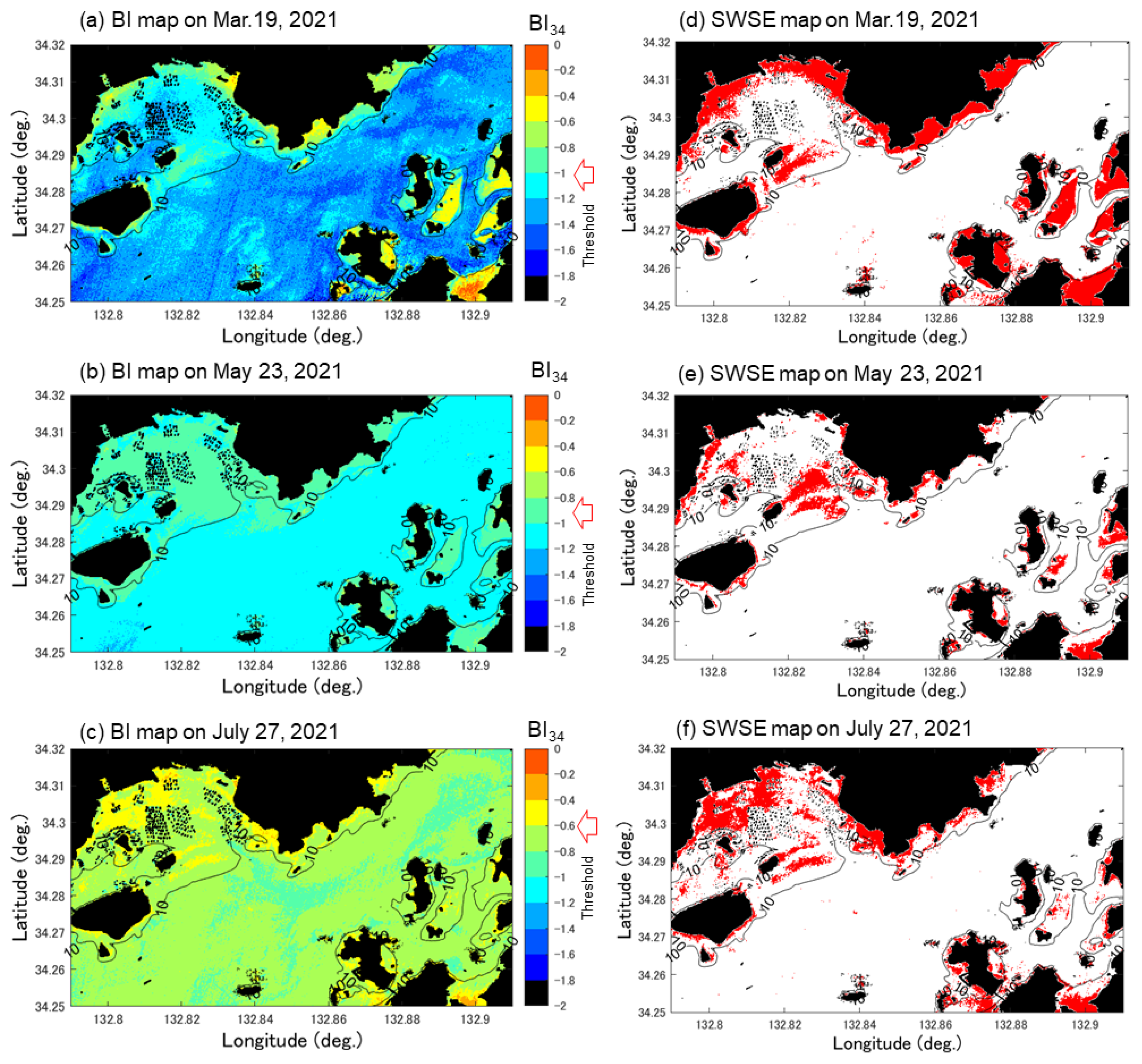
4.1. Validity of Underwater Forest Area Selection Using Bottom Index

This section discusses the validity of the marine forest distribution map of the study area based on the BI method shown in Figure 6a,b. As mentioned previously, marine forests in the Seto Inland Sea occur at depths of less than 10 m. The BI method used in this study included the SWSG bed distribution maps presented in Figure 12b and Figure 13c, which were measured SWSG bed distribution maps over almost the entire area. Thus, it was judged to be appropriate in that respect. However, in general, the setting of k_ij (or the combination of bands) in Equation (9) is crucial when applying the BI method. Herein, the combination of Band 3 (green band) and Band 4 (red band) of Sentinel-2, which had a high correlation coefficient, was adopted. However, depending on the environment, a combination of blue and green bands is also effective [29]. This is because short wavelengths, which are more transparent, are effective in clean waters, such as coral reefs. However, in eutrophic waters, such as the Seto Inland Sea, absorption by color-dissolved organic matter (CDOM) in the blue band is relatively large owing to the strong absorption of CDOM and chlorophyll derived from rivers and sediments. Consequently, their absorption effects were weaker and the green and red bands appeared to be more effective. Moreover, upon the application of Terra ASTER (Advanced Spaceborne Thermal Emission and Reflection Radiometer)’s green and red bands to BI in the same region, they were effective in mapping Zostera beds [30], confirming the validity of the present results. Moreover, the potential monthly carbon storage amounts were estimated. According to the UNEP report [31], the average storage rate per unit area of seagrass is 0.83 carbon t/ha/year, with a range of 0.56 to 1.82 carbon t/ha/year. Applying these rates, the estimated carbon sequestration in our study area was found to be 53.08 t in March, 62.43 t in May, and 48.64 t in July [31,32]. It is important to note that the area of seagrass beds in the Seto Inland Sea decreased between 1960 and 1991, but has recently experienced revival due to improvements in water quality [31]. This highlights the significance of water quality improvement in enhancing the carbon sequestration capacity of seagrasses.

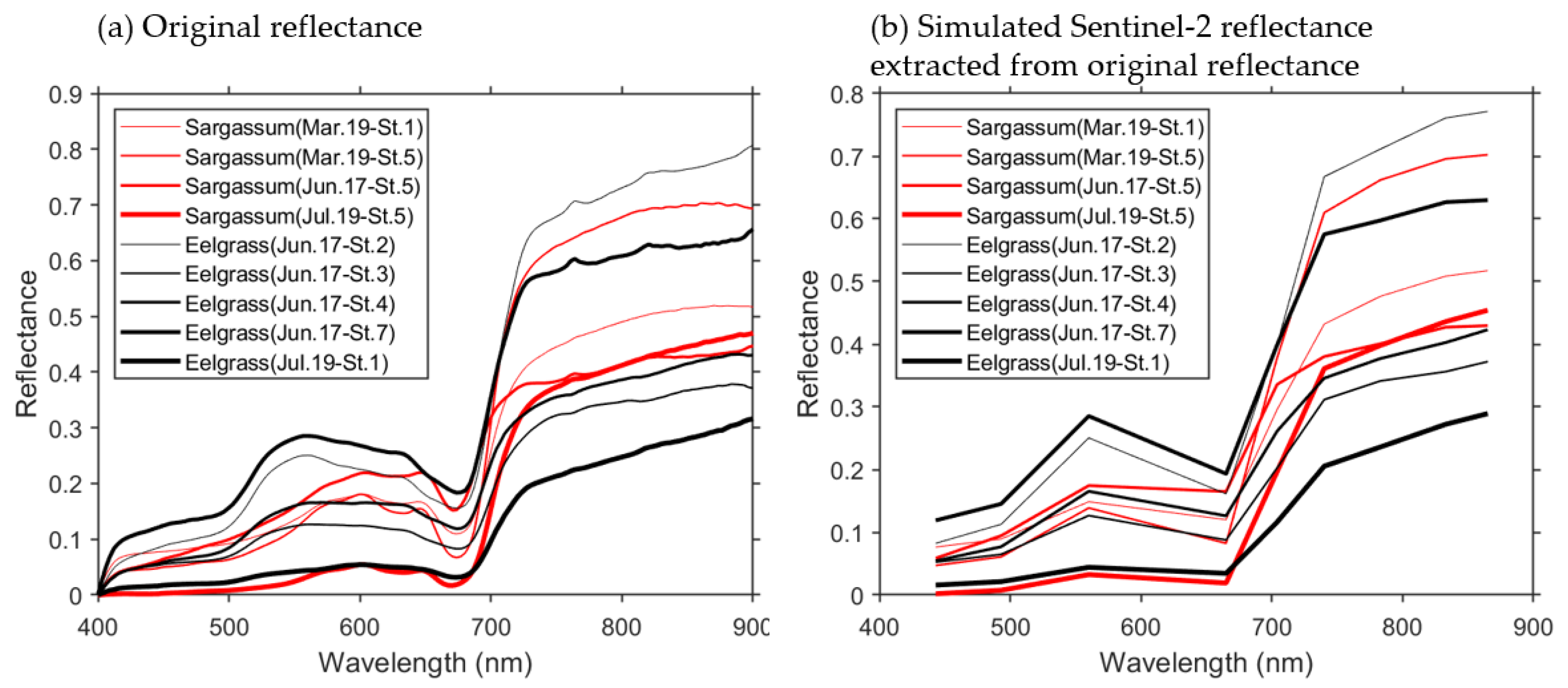
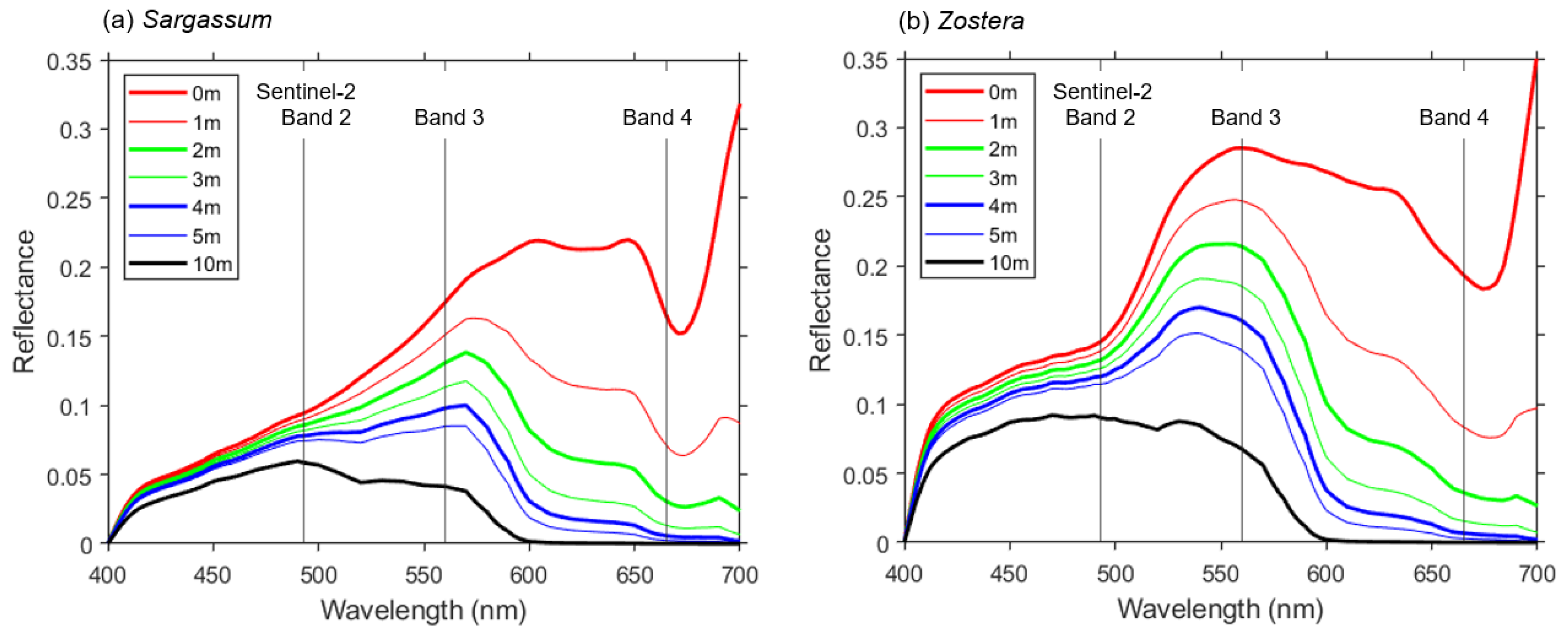
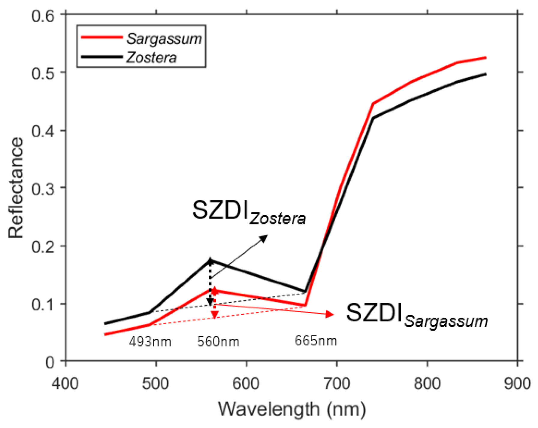
4.2. Spectral Characteristics of Zostera and Sargassum

This section discusses the spectral reflectance characteristics of Sargassum and Zostera in the target area, as shown in Figure 7. In this study, the differences in the spectral characteristics of Sargassum and Zostera can be approximately summarized as blue (400–500 nm), with low reflectance for both, red band (610–650 nm) for Zostera, and green band (550–560 nm) for Sargassum. This feature is also evident from the fact that the photographs of Sargassum and Zostera in Figure 3 appeared red and green, respectively. Upon further examining the reflectance characteristics, the present results showed that the reflectance for Sargassum was low in blue (400–500 nm) and in green (500–600 nm), and was high in near red (610 and 650 nm), compared to Zostera.

Previous studies on the spectral reflectance characteristics of these species include those on seagrass Zostera capricorni, Posidonia australis, and Halophila ovalis in eastern Australian waters [26] and the seagrass Thalassia in southern Florida [33]. Furthermore, studies on the green algae Ulva on the coast of China by Shin et al. [34] and Sargassum species in the Gulf of Mexico and the Atlantic Ocean by Hu et al. [19] represent other such research. For example, from past spectroscopic studies on Sargassum, Sargassum is known to be a type of brown macroalgae that contains the accessory pigments fucoxanthin and chlorophyll c [35]. The bio-absorption peaks of fucoxanthin are at blue and green wavelengths (480 and 520 nm). Additionally, chlorophyll c exhibits absorption peaks at blue (460 and 485 nm) and red (635 nm) [35,36] wavelengths. Conversely, the Zostera leaf and syringodium wrack contain chlorophyll b, with absorption peaks at blue and red wavelengths (470, 600, and 650 nm) [35]. To summarize these past studies, the spectral reflectance characteristics of Sargassum and Zostera are low for blue (460, 470, and 480 nm) wavelengths. A low reflectance at green (520 nm) wavelengths for Sargassum and a low reflectance for Zostera at red (600, 635, and 650 nm) wavelengths have also been confirmed. This indicates that the fundamental characteristics of Sargassum and Zostera in this study area are consistent with the characteristics of Zostera around the world.

4.3. Validity and Limitations of the SZDI Method

This section discusses the validity and limitations of the SZDI method, as shown in Figure 9 and Equations (10) and (11). As mentioned in Section 4.2, the definitive spectral characteristics of Zostera and Sargassum were characterized by a maximum near red (610 nm and 650 nm) wavelength for Sargassum and a minimum at ~630 nm for Zostera. Thus, it is desirable to use an index, such as the ratio of green to red, to separate Zostera and Sargassum. Dierssen et al. [35] proposed the ratio of reflectance values at 650 and 630 nm as the Sargassum index (SI). However, Sentinel-2 does not observe these bands (particularly the 630 nm band), and when considering only the Sentinel-2 bands, as shown in Figure 7b, the sentinel-2 reflectance does not necessarily reflect the green reflectance of Sargassum. The red area is not necessarily higher than the green area. Rather, the difference in the green reflectance appeared to be more useful for separation. Furthermore, by emphasizing the contrast with the reflectance of the background water, the difference in the green reflectance became clearer and more helpful when employed to distinguish Sargassum and Zostera. Considering all these ideas, Equations (10) and (11) (applicable to the FAI) [20,33] were considered to be effective methods for separating Sargassum and Zostera. This method, as summarized in Figure 9, calculated the baseline reflectance obtained using Band 2 (480 nm) and Band 4 (655 nm) from Sentinel-2 Band 3 (560 nm) reflectance. The higher the value, the more likely it was to be Zostera, whereas the lower the value, the more likely it was to be Sargassum. When the SZDI was calculated using Equations (10) and (11) and mapped using the thresholds set, as shown in Figure 10, seasonal distribution changes were evident. Furthermore, the distribution indicates that Zostera thrives in shallow sandy areas, while Sargassum prefers comparatively deeper, rocky, and intertidal zones, aligning well with their biological characteristics. In the Seto Inland Sea, Sargassum is predominantly composed of three species: S. condusum, S. yezoense, and S. trichophyllum, with maturity periods spanning from March to June, June to August, and October to December, respectively [20]. These findings contribute to explaining the rationale for the presence of Sargassum in our study during the period from March to July. Some studies also suggest that Zostera matures in June and experiences a decline thereafter [37], supporting our result that Zostera occupied the largest area in the May image but decreased in the July image. In conclusion, the distribution not only exhibits a high level of consistency with the optical characteristics of Sargassum and Zostera, but also aligns closely with the findings from our field survey, as presented in Table 5 and the data provided by the MOEJ in Figure 12. Additionally, it resonates with the biological attributes of both Sargassum and Zostera.

However, at present, this method has certain limitations. One limitation is the influence of water depth z and k on Equation (3) within the SWSG bed area extracted using the BI method. Nevertheless, the reason why the seasonal changes in Zostera and Sargassum were valid (Figure 11) can be attributed to the assumptions or water depth correction method being effective to a certain extent during the analysis period. However, in reality, the spectrum of SWSG considerably changes depending on chlorophyll a and turbidity, which greatly affects k. Thus, to improve the accuracy of SWSG classification, the water quality information at the time of observation must be considered and the SWSG must be reflected. Furthermore, the rate may require correction. Meanwhile, in situations where the seagrass develops to maturation and releases floating seaweed, the upper seagrass may cover the lower seagrass, rendering the lower seagrass undetectable. Another challenge lies in the difficulty of achieving precise mathematical verification at present. In fact, there has only been one existing field survey conducted by the Ministry of the Environment, Government of Japan, primarily due to economic and time constraints; this was in 2014. Thus, there appears to be a lack of precise mathematical verification at present. To address these issues, the use of a hyperspectral sensor or the strategic design of a field survey tailored to match the satellite image of the specific area beforehand could be considered.

5. Conclusions

This study proposed a method for separating Sargassum and Zostera in the Seto Inland Sea using Sentinel-2 data and examined the validity of the method. Consequently, the following points were clarified.

• The BI method was an effective method, using a combination of Band 3 (green) and Band 4 (red) Sentinel-2 data for estimating the area of SWSG beds in the sea.
• The spectral reflectance characteristics of Sargassum and Zostera measured on site were understood. In general, the characteristics exhibit low reflectance in the blue and red bands for both Sargassum and Zostera, but exhibit relative high reflectance in the green band for Zostera.
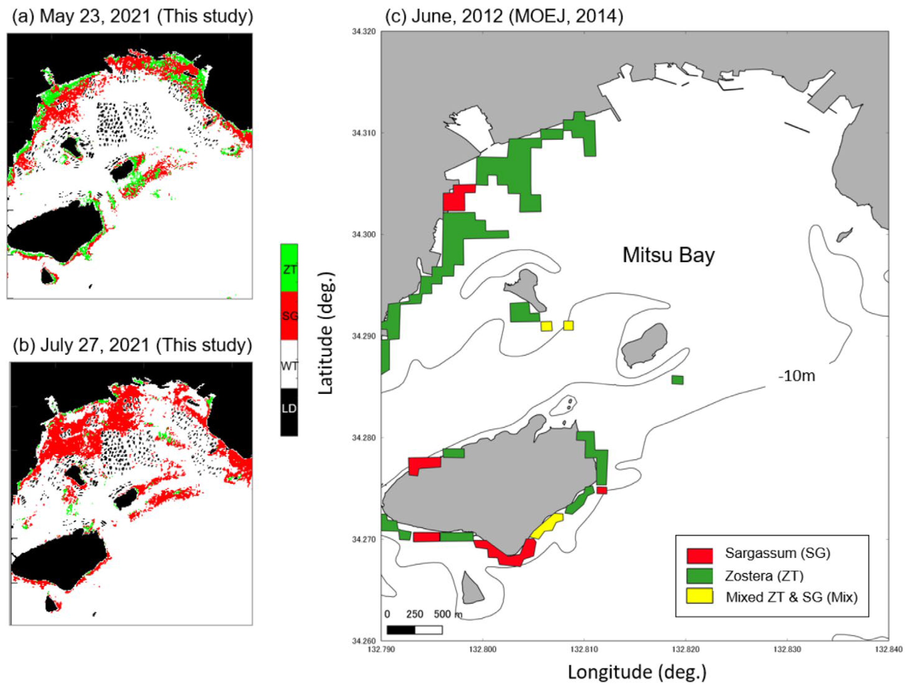
• The SZDI, which used the height from the background of Sentinel-2 Band 3 (560 nm) as an index, was proposed as a method for separating Sargassum and Zostera. Its validity was confirmed through field surveys, the examination of past SWSG bed maps, and the consideration of biological characteristics.

In the future, we will improve methods for automatically determining BI thresholds, which are currently determined by trial and error. Furthermore, we intend to promote classification methods that use artificial intelligence and hyperspectral sensors, which have been rapidly developed in recent years, to classify kelp and green algae in addition to Sargassum and Zostera beds.

References

1. Smith, S.V. Marine Macrophytes as a Global Carbon Sink. Science 1981, 211, 838–840. [Google Scholar] [CrossRef] [PubMed]
2. Greiner, J.T.; McGlathery, K.J.; Gunnell, J.; McKee, B.A. Seagrass Restoration Enhances “Blue Carbon” Sequestration in Coastal Waters. PLoS ONE 2013, 8, e72469. [Google Scholar] [CrossRef] [PubMed]
3. Lavery, P.S.; Mateo, M.-Á.; Serrano, O.; Rozaimi, M. Variability in the Carbon Storage of Seagrass Habitats and Its Implications for Global Estimates of Blue Carbon Ecosystem Service. PLoS ONE 2013, 8, e73748. [Google Scholar] [CrossRef] [PubMed]
4. Tokoro, T.; Hosokawa, S.; Miyoshi, E.; Tada, K.; Watanabe, K.; Montani, S.; Kayanne, H.; Kuwae, T. Net Uptake of Atmospheric CO2 by Coastal Submerged Aquatic Vegetation. Glob. Chang. Biol. 2014, 20, 1873–1884. [Google Scholar] [CrossRef]
5. Ministry of the Environment. Available online: https://www.env.go.jp/water/heisa/setonaikai_law_rev.html (accessed on 9 November 2023).
6. Yamamoto, T. The Seto Inland Sea––Eutrophic or Oligotrophic? Mar. Pollut. Bull. 2003, 47, 37–42. [Google Scholar] [CrossRef]
7. Imai, I.; Yamaguchi, M.; Hori, Y. Eutrophication and Occurrences of Harmful Algal Blooms in the Seto Inland Sea, Japan. Plankton Benthos Res. 2006, 1, 71–84. [Google Scholar] [CrossRef]
8. Takeoka, H. Progress in Seto Inland Sea Research. J. Oceanogr. 2002, 58, 93–107. [Google Scholar] [CrossRef]
9. Dierssen, H.M.; Zimmerman, R.C.; Leathers, R.A.; Downes, T.V.; Davis, C.O. Ocean Color Remote Sensing of Seagrass and Bathymetry in the Bahamas Banks by High-Resolution Airborne Imagery. Limnol. Oceanogr. 2003, 48, 444–455. [Google Scholar] [CrossRef]
10. Traganos, D.; Reinartz, P. Mapping Mediterranean Seagrasses with Sentinel-2 Imagery. Mar. Pollut. Bull. 2018, 134, 197–209. [Google Scholar] [CrossRef]
11. Lyzenga, D.R. Passive Remote Sensing Techniques for Mapping Water Depth and Bottom Features. Appl. Opt. 1978, 17, 379. [Google Scholar] [CrossRef]
12. Lyzenga, D.R. Remote Sensing of Bottom Reflectance and Water Attenuation Parameters in Shallow Water Using Aircraft and Landsat Data. Int. J. Remote Sens. 1981, 2, 71–82. [Google Scholar] [CrossRef]
13. Philpot, W.D. Bathymetric Mapping with Passive Multispectral Imagery. Appl. Opt. 1989, 28, 1569. [Google Scholar] [CrossRef] [PubMed]
14. Stumpf, R.P.; Holderied, K.; Sinclair, M. Determination of Water Depth with High-Resolution Satellite Imagery over Variable Bottom Types. Limnol. Oceanogr. 2003, 48, 547–556. [Google Scholar] [CrossRef]
15. Biodiversity Center of Japan. Available online: https://www.biodic.go.jp/moba/1_1.html (accessed on 20 September 2023). (In Japanese)
16. Gower, J.; Hu, C.; Borstad, G.; King, S. Ocean Color Satellites Show Extensive Lines of Floating Sargassum in the Gulf of Mexico. IEEE Trans. Geosci. Remote Sens. 2006, 44, 3619–3625. [Google Scholar] [CrossRef]
17. Hu, C. A Novel Ocean Color Index to Detect Floating Algae in the Global Oceans. Remote Sens. Environ. 2009, 113, 2118–2129. [Google Scholar] [CrossRef]
18. Gower, J.F.R.; King, S.A. Distribution of Floating Sargassum in the Gulf of Mexico and the Atlantic Ocean Mapped Using MERIS. Int. J. Remote Sens. 2011, 32, 1917–1929. [Google Scholar] [CrossRef]
19. Hu, C.; Feng, L.; Hardy, R.F.; Hochberg, E.J. Spectral and Spatial Requirements of Remote Measurements of Pelagic Sargassum Macroalgae. Remote Sens. Environ. 2015, 167, 229–246. [Google Scholar] [CrossRef]
20. Yoshida, T. Japanese species of Sargassum subgenus Bactrophycus (Phaeophyta, Fucales). J. Fac. Sci. Hokkaido Univ. Ser. 5 Bot. 1983, 13, 99–246. [Google Scholar]
21. Yoshida, G.; Hori, M.; Sakiyama, K.; Hamaguchi, M.; Kajita, A.; Nishimura, K.; Shoji, J. Distribution of Seaweed Bed and Tidal Flat and Their Correlations with Fisheries Catches in the Nine Sea Areas of the Seto Inland Sea. Fish. Eng. 2010, 47, 19–29. [Google Scholar]
22. Albert, A.; Mobley, C. An Analytical Model for Subsurface Irradiance and Remote Sensing Reflectance in Deep and Shallow Case-2 Waters. Opt. Express 2003, 11, 2873. [Google Scholar] [CrossRef]
23. Odagawa, S.; Takeda, T.; Yamano, H.; Matsunaga, T. A Proposed Method for Estimation of Cover Degree for Each Bottom-Type in Coral Reef Areas Using Hyperspectral Data. J. Remote Sens. Soc. Jpn. 2016, 36, 1–10. [Google Scholar] [CrossRef]
24. Morel, A.; Prieur, L. Analysis of Variations in Ocean Color1. Limnol. Oceanogr. 1977, 22, 709–722. [Google Scholar] [CrossRef]
25. Matsunaga, T.; Hoyano, A.; Mizukami, Y. Spatial/temporal variation of sea water extinction coefficient ratio and temporal change detection in coral reef using bottom index. In Proceedings of the 26th Japanese Conference on Remote Sensing, Hanoi, Vietnam, 7–11 November 2005; pp. 281–282. [Google Scholar]
26. Qi, L.; Hu, C.; Wang, M.; Shang, S.; Wilson, C. Floating Algae Blooms in the East China Sea. Geophys. Res. Lett. 2017, 44, 501–511. [Google Scholar] [CrossRef]
27. Ministry of the Environment; Biodiversity Center of Japan. Marine Biotic Survey (Coral Reef Survey), in the 4th National Survey on the Natural Environment. 1991. Available online: http://www.biodic.go.jp/reports2/4th/coralreef/4_coralreef.pdf (accessed on 20 September 2023). (In Japanese)
28. Ministry of the Environment; Government of Japan. Mitsu Bay Area Healthy Plan. 2014. Available online: https://www.env.go.jp/water/heisa/healthyplan/attach/healthyplan-mitsu_b-1.pdf (accessed on 20 September 2023). (In Japanese)
29. Kakuta, S.; Takeuchi, W.; Prathep, A. Seaweed and Seagrass Mapping in Thailand Measured Using Landsat 8 Optical and Textural Image Properties. J. Mar. Sci. Technol. 2016, 24, 13. [Google Scholar] [CrossRef]
30. Sochea, L.; Sakuno, Y. Eelgrass Bed Monitoring Using Satellite Terra/Aster Data in Yoshina Tidal Flat. Proc. Hydraul. Eng. 2008, 52, 1381–1386. [Google Scholar] [CrossRef]
31. Hori, M.; Bayne, C.J.; Kuwae, T. Blue Carbon: Characteristics of the Ocean’s Sequestration and Storage Ability of Carbon Dioxide. In Blue Carbon in Shallow Coastal Ecosystems; Kuwae, T., Hori, M., Eds.; Springer Singapore: Singapore, 2019; pp. 1–31. ISBN 9789811312946. [Google Scholar]
32. Nellemann, C.; Corcoran, E. Blue Carbon: The Role of Healthy Oceans in Binding Carbon: A Rapid Response Assessment; UNEP/Earthprint: Nairobi, Kenya, 2009. [Google Scholar]
33. Thorhaug, A.; Richardson, A.D.; Berlyn, G.P. Spectral Reflectance of Thalassia testudinum (Hydrocharitaceae) Seagrass: Low Salinity Effects. Am. J. Bot. 2006, 93, 110–117. [Google Scholar] [CrossRef]
34. Shin, J.; Lee, J.-S.; Jang, L.-H.; Lim, J.; Khim, B.-K.; Jo, Y.-H. Sargassum Detection Using Machine Learning Models: A Case Study with the First 6 Months of GOCI-II Imagery. Remote Sens. 2021, 13, 4844. [Google Scholar] [CrossRef]
35. Dierssen, H.M.; Chlus, A.; Russell, B. Hyperspectral Discrimination of Floating Mats of Seagrass Wrack and the Macroalgae Sargassum in Coastal Waters of Greater Florida Bay Using Airborne Remote Sensing. Remote Sens. Environ. 2015, 167, 247–258. [Google Scholar] [CrossRef]
36. Orzymski, J.; Johnsen, G.; Sakshaug, E. The Significance of Intracellular Self-Shading on the Biooptical Properties of Brown, Red, and Green Macroalgae. J. Phycol. 1997, 33, 408–414. [Google Scholar] [CrossRef]
37. Fujiwara, M. Research on Appropriate Creation Technology for Zostera Beds in and around the Coastal Shallow Areas, Seto-Inland Sea. Bull. Kagawa Pref. Fish. Exp. Stn. 2013, 14, 1–51. [Google Scholar]
Figure 1. Study area depicting field survey points and water depth. This image is extracted from the yellow square in the top left corner. St. 1–St. 8 indicate the locations where we conducted field survey.
Water 15 03979 g001
Figure 2. Flow chart of the study method employed.
Water 15 03979 g002
Figure 3. Sargassum (left) and Zostera (right) were obtained locally. The bottom photograph is a snapshot of an underwater video image of the seagrass, and the top photograph is of the seagrass, hoisted on board.
Water 15 03979 g003
Figure 4. Reshaped Bottom topographic distribution map based on the M7000 series (https://www.jha.or.jp/en/jha/, accessed on 9 November 2023).
Water 15 03979 g004
Figure 5. Scatterplots of Sentinel-2 Band 2–3 and Band 3–4 at the sand area of two river mouth sites for determining the extinction coefficient ratio. In (a), the upper plot illustrates the natural logarithm ratio between band 2–3, while the lower plot shows the natural logarithm ratio between band 3–4 on 19 March 2021. (b) shows the natural logarithm ratio on 23 May 2021, and (c) shows the ratio on 27 July 2021.
Water 15 03979 g005
Figure 6. Bottom index (BI) map (ac) and SWSG map (df) extracted from BI map on 19 March, 23 May, and 27 June 2021, as estimated from Sentinel-2 data.
Water 15 03979 g006
Figure 7. Spectral reflectance of Sargassum and Zostera obtained through field survey. Red and black indicate Sargassum and Zostera, respectively. (a) indicates the original reflectance and (b) indicates the simulated Sentinel-2 reflectance extracted from original reflectance.
Water 15 03979 g007
Figure 8. Simulated spectral reflectance of Sargassum and Zostera depending on water depth. (a) Sargassum at St. 5 on 17 June 2021. (b) Zostera at St. 7 on 17 June.
Water 15 03979 g008
Figure 9. Schematic of the proposed Sargassum and Zostera distinguishing index (SZDI) of Sentinel-2 bands.
Water 15 03979 g009
Figure 10. Distribution maps of Sargassum and Zostera on 19 March, 23 May, and 27 July 2021. The green and orange colors represent Zostera (EL) and Sargassum (SG), respectively. The white and gray colors represent sea water (WT) and land (LD), respectively. (ac) represents SZDI maps on 19 March, 23 May, and 27 July 2021. (df) represents Sargassum and Zostera maps obtained after applying the determined threshold of SZDI.
Water 15 03979 g010
Figure 11. SZDI (Sargassum and Zostera Distinguish Index) threshold setting results.
Water 15 03979 g011
Figure 12. Comparison of Sargassum and Zostera distribution maps and Sentinel-2 map in this study. (a) and the redrawn reference map based on Ministry of the Environment, Government of Japan (1991) data. Black isoline in (b) indicates a 10 m water depth. A, B, and C are three water areas marked for convenient verification discussion.
Water 15 03979 g012
Figure 13. Comparison of Sargassum and Zostera distribution maps and Sentinel-2 maps both in May (a) and July (b) in the Mitsu Bay and redrawn reference map (c) based on the field work by Ministry of the Environment, Government of Japan (2014). Black isoline in (c) indicates 10 m water depth.
Water 15 03979 g013
Figure 14. Temporal change in marine forest areas in this study area, derived from Sentinel-2 data.
Water 15 03979 g014