

Flood Forecasting by Using Machine Learning: A Study Leveraging Historic Climatic Records of Bangladesh
 , ,
, ,  ,
,  and
and
Abstract
:1. Introduction
- Highlight the serious and long-lasting effects that floods have on the socioeconomic system, agriculture, and human life while acknowledging the growing challenge in accurately estimating rainfall because of climatic changes, non-linear qualities, and variable attributes.
- Suggest a combined approach for data with computationally intensive flood channel mathematical models to predict flooding levels and velocities across a wide area.
- Identify undetected trends in historical meteorological data to identify machine learning and deep learning approaches as valuable tools for precisely estimating rainfall with quantitative results to prove the usefulness of the machine learning models.
- Implement evaluation measures to assess the efficiency and progress made by the machine learning models, such as the R2 score and root mean squared error.
- Observation that the random forest regressor and k-nearest neighbours algorithms achieved high accuracy, 96% and 99%, respectively.
2. Literature Review
2.1. Related Work
2.2. Discussion on Past Studies
- Classical meteorological systems: In the past, physical-based models like the HEC-HMS, SWAT, and MIKE SHE predominated flood forecasting. These representations incorporate physical equations that represent the flow and accumulation of water [2].
- Mathematical Models based on statistics: The exponential smoothing and ARIMA statistical analysis of time series techniques were also employed to anticipate river flows and flood levels. These techniques rely on the data’s statistical patterns [62].
- Incorporation of machine learning techniques: Machine learning techniques have become more prevalent in recent years. Investigations have demonstrated that when there are a lot of data available, machine learning can frequently match or even surpass conventional hydrological projections [63].
- Numerous studies rely on small or sparse datasets, which might not fully account for all possible flood situations. Records for extreme occurrences or isolated flooding disasters are frequently lacking. Climatic datasets are often incomplete and inaccurate, particularly in nations with limited resources.
- Several models are inefficient when used differently because they are overfit to datasets or areas. Model portability between several geographic areas is still rugged.
- Numerous ML models, intense learning models, behave as “black boxes”, making it challenging to comprehend how they make decisions. This makes it difficult to win over the trust of stakeholders and end users.
- When ML models are combined with conventional meteorological models, which have been widely used and relied upon for years, there is frequently a gap. The physical processes that play a role in flood generation and propagation are not always adequately taken into consideration in studies.
- For real-time prediction, the computational burden of some sophisticated ML models may be too high. Specific models could be useless in time-sensitive situations due to the time required for data collection, initial processing, and forecasting.
- Certain approaches might be practical in local watersheds or urban areas, but they might have difficulties when scaled up to substantial river valleys.
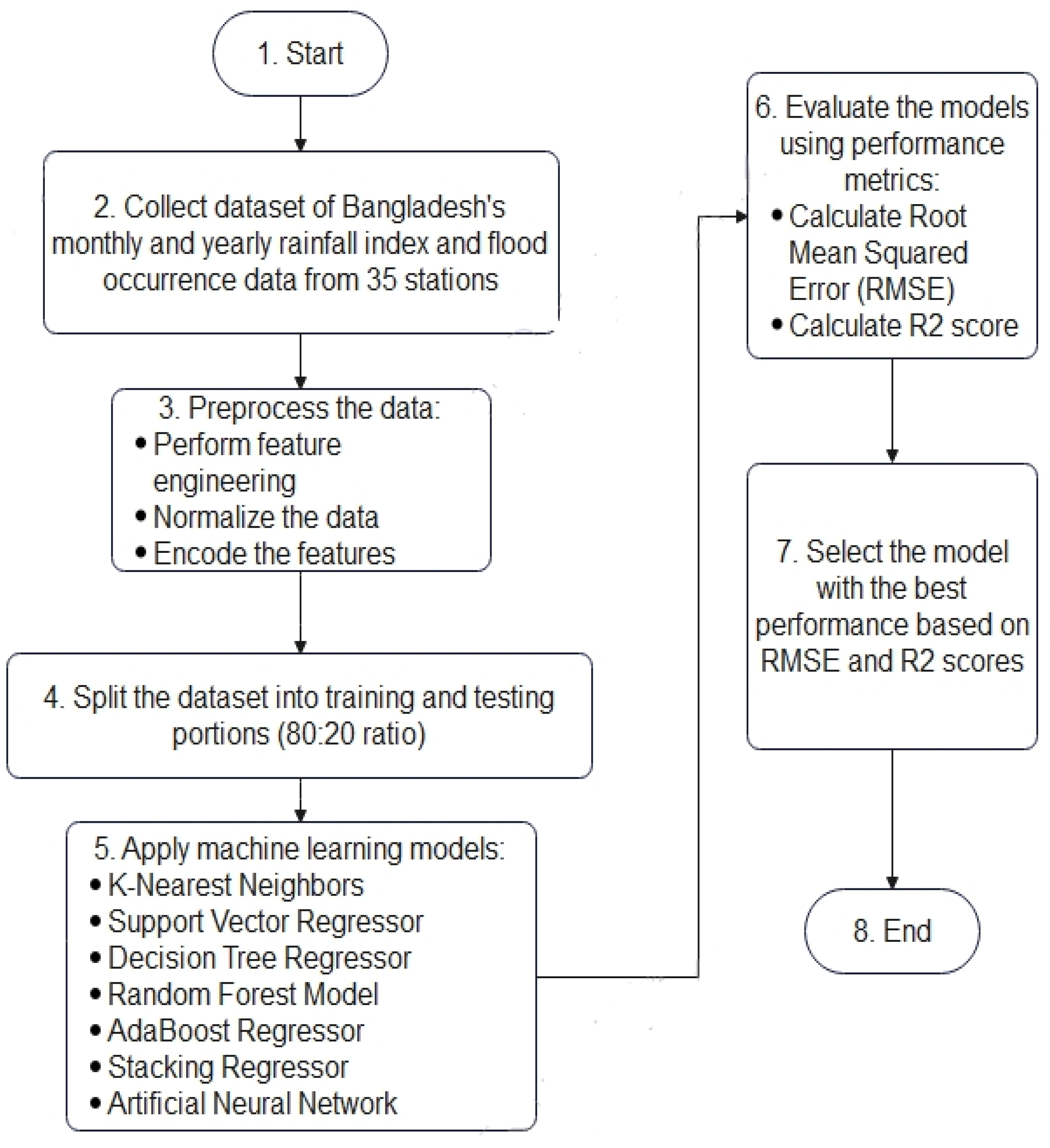
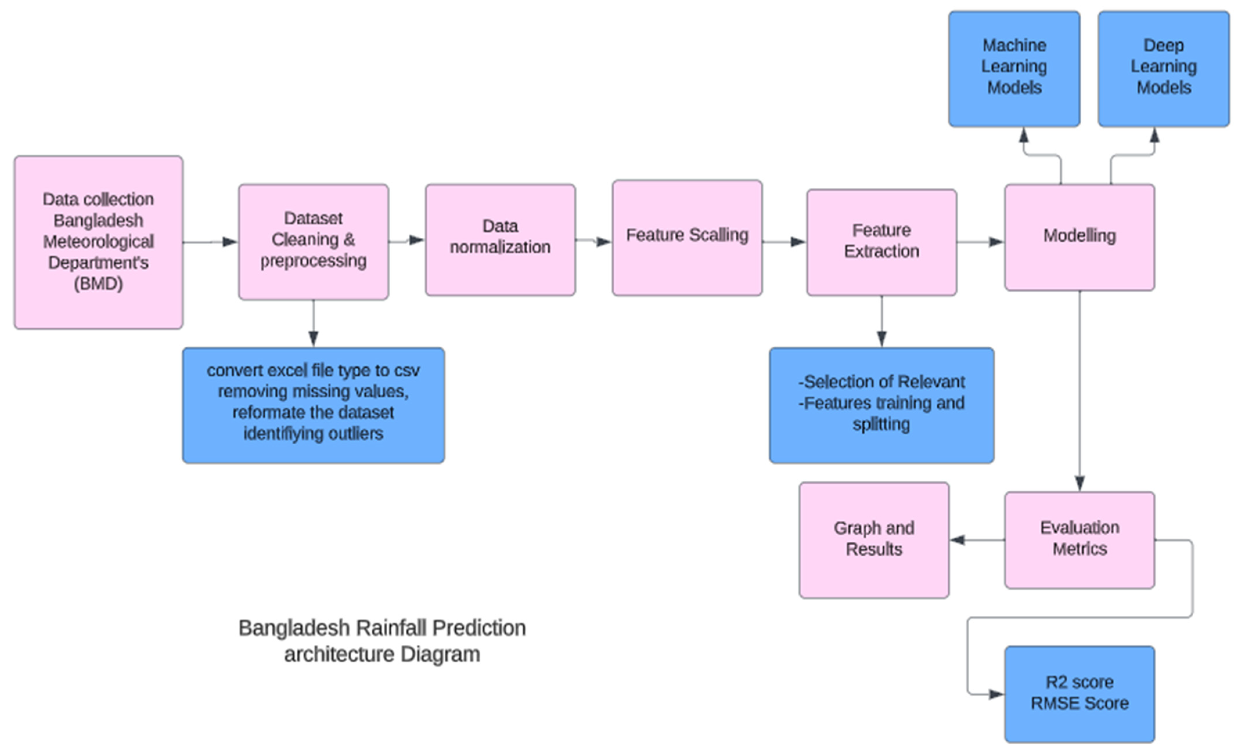
3. Proposed Methodology
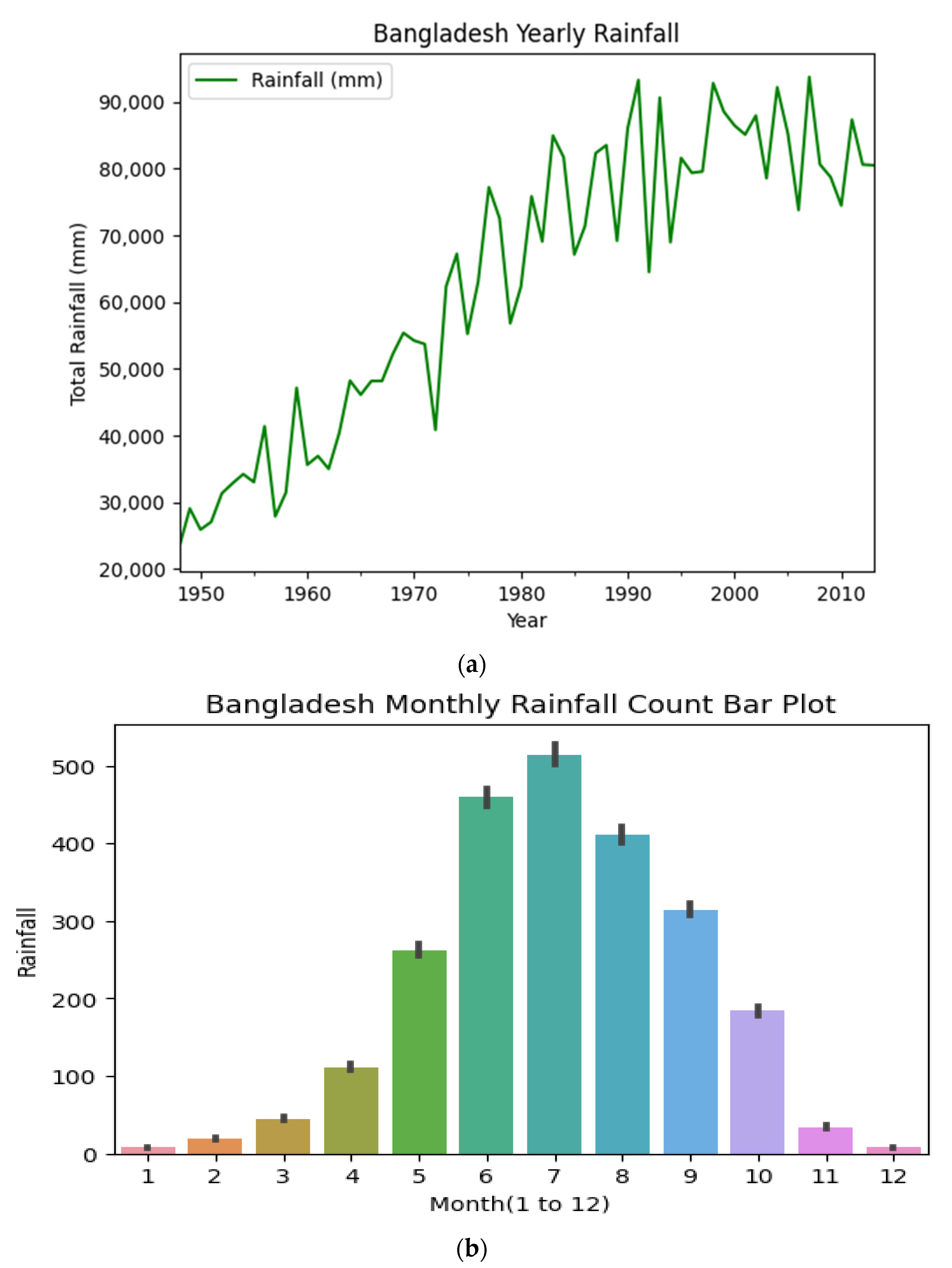
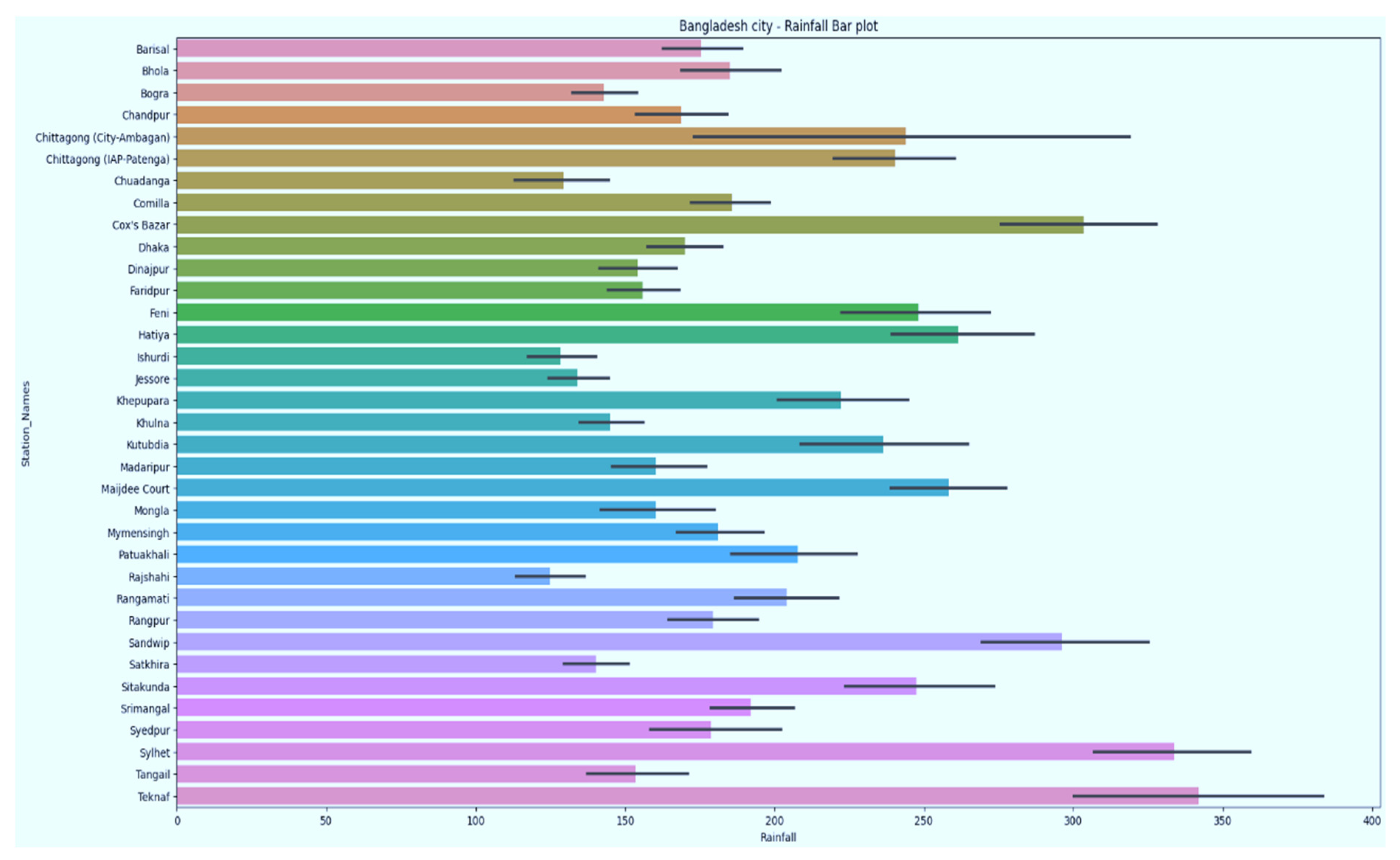
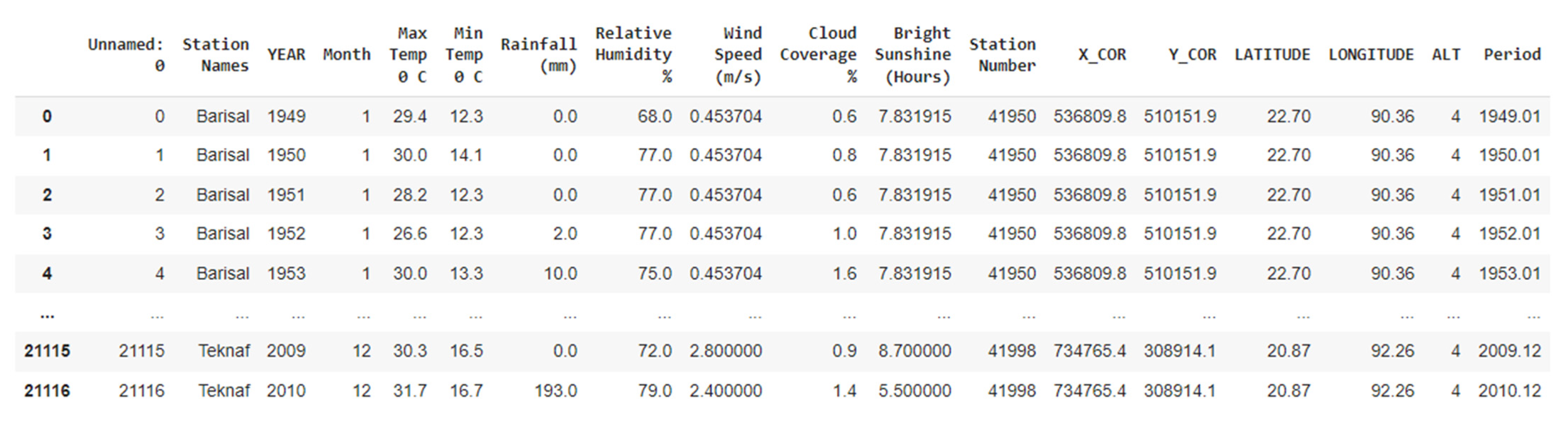
3.1. Dataset Description
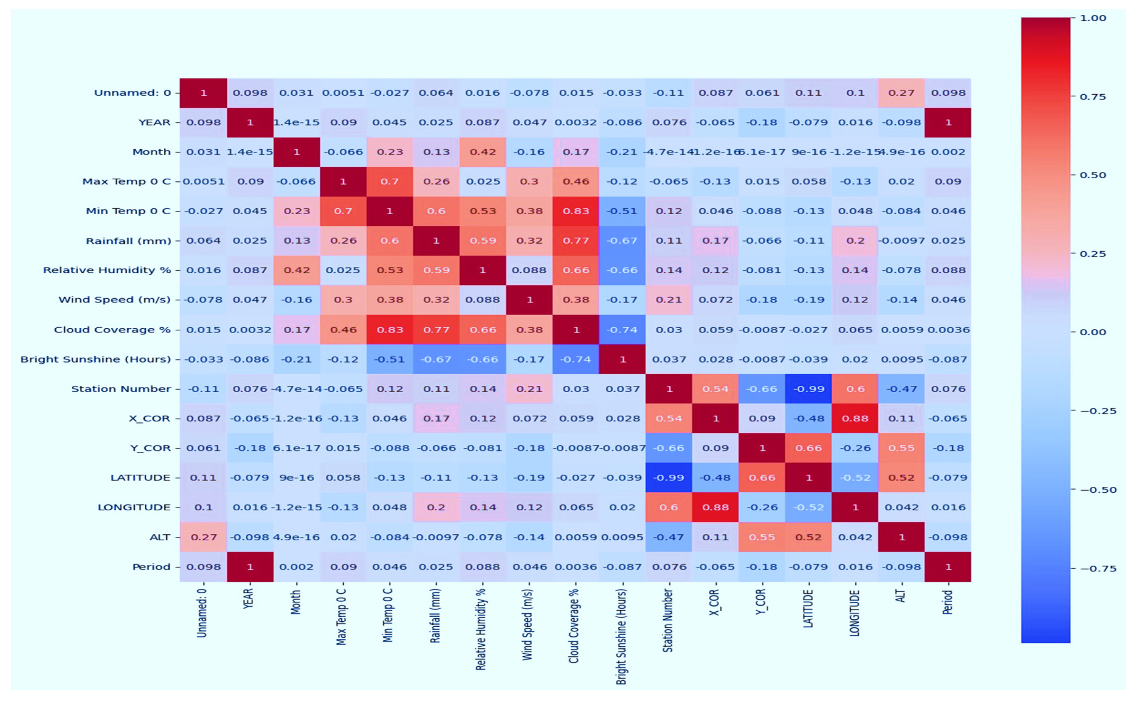
3.2. Dataset Preprocessing or Cleaning
- YEAR: This represents the year;
- X_COR: This represents the x-coordinate where rainfall is happening;
- Y_COR: This represents the y-coordinate;
- LATITUDE: The latitude of the location;
- LONGITUDE: The longitude of the location;
- ALT: The altitude of the location.
3.3. Data Normalisation
3.4. Feature Encoding
3.5. Feature Scaling
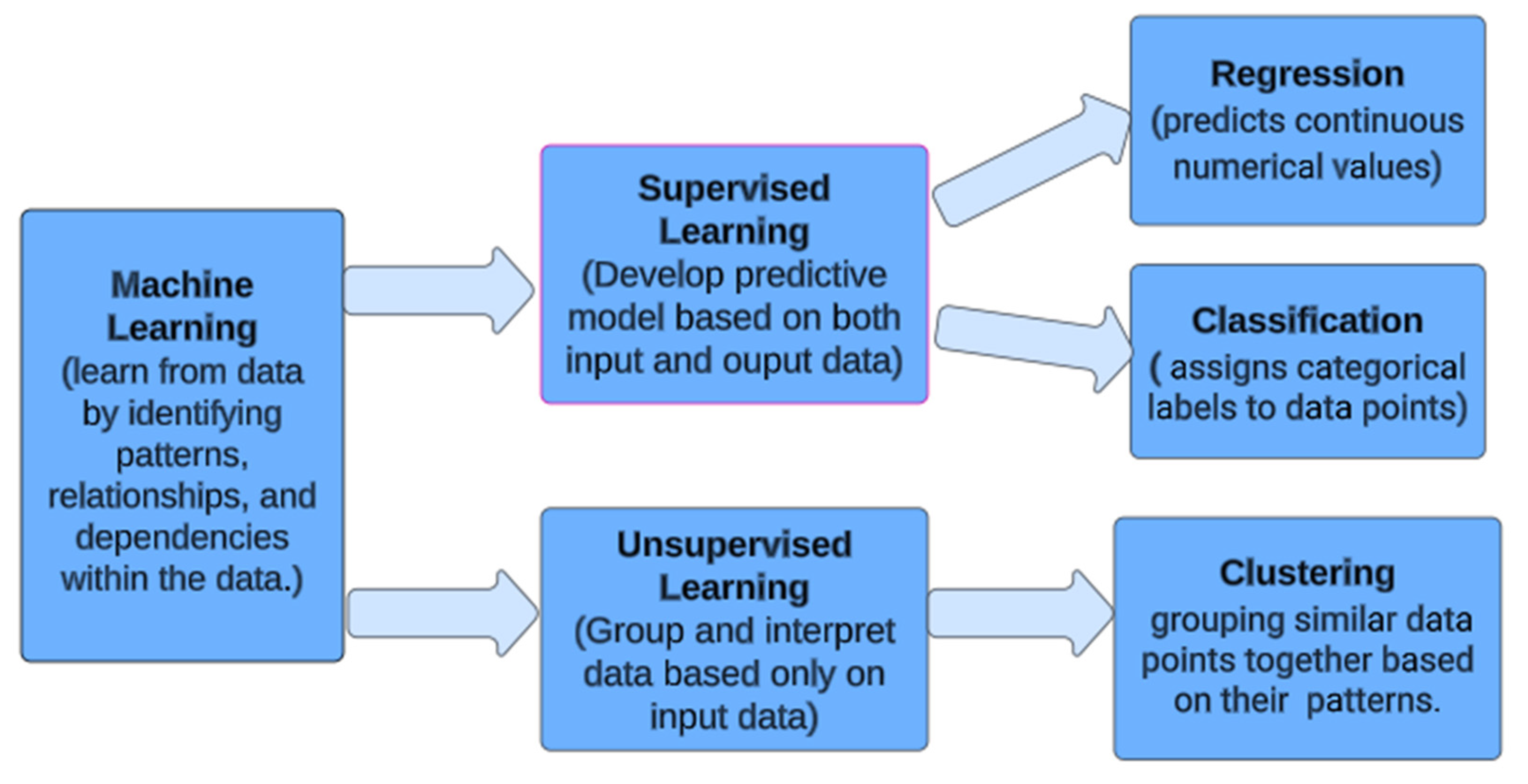
3.6. Machine Learning Models
3.6.1. Polynomial Linear Regression
3.6.2. Multiple Linear Regression
3.6.3. K-Nearest Neighbours Regressor
3.6.4. Decision Tree Regressor
3.6.5. Support Vector Machine
3.6.6. Random Forest Model
3.6.7. AdaBoostRegressor
3.6.8. Stacking Regressor
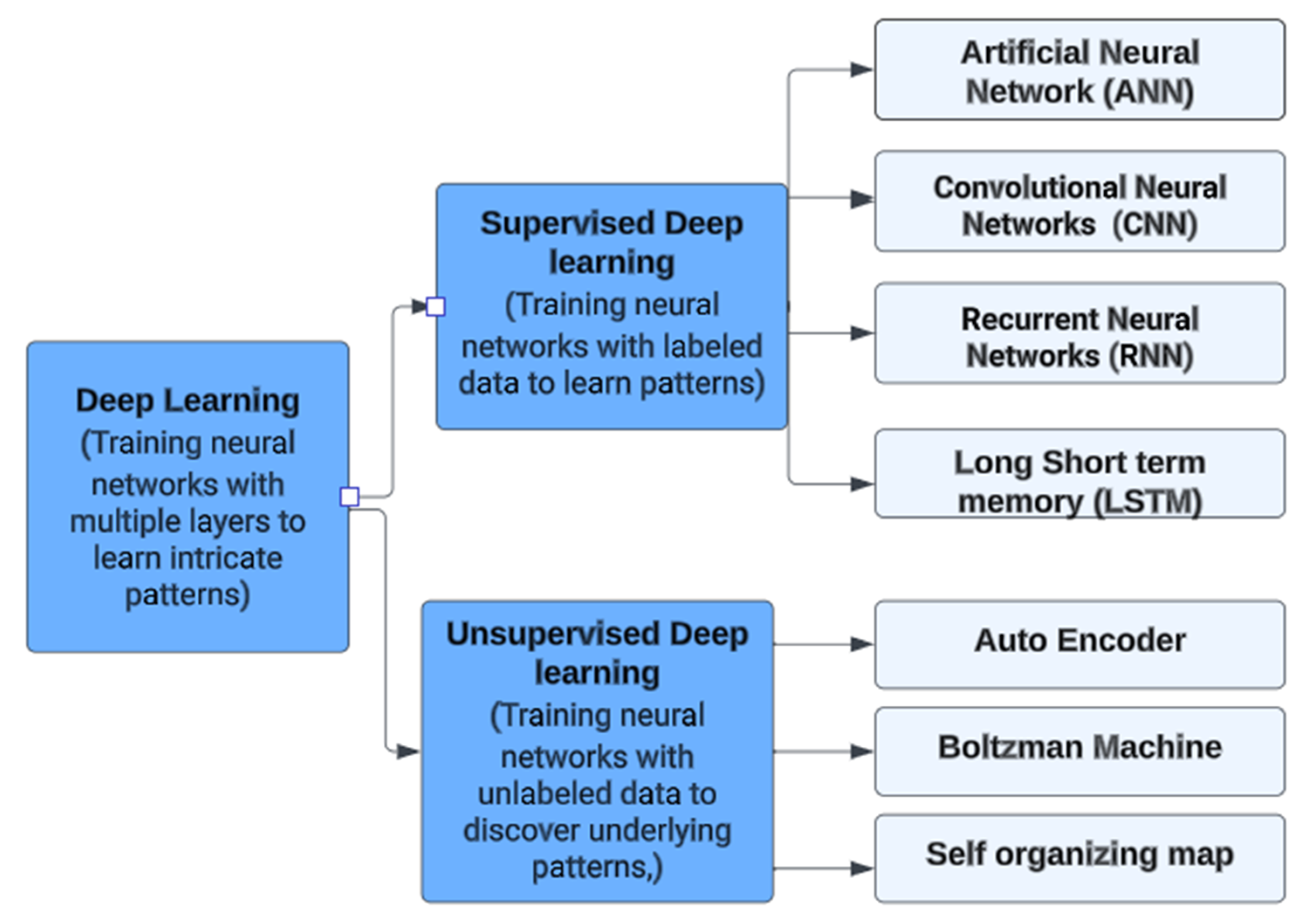
3.7. Deep Learning Model
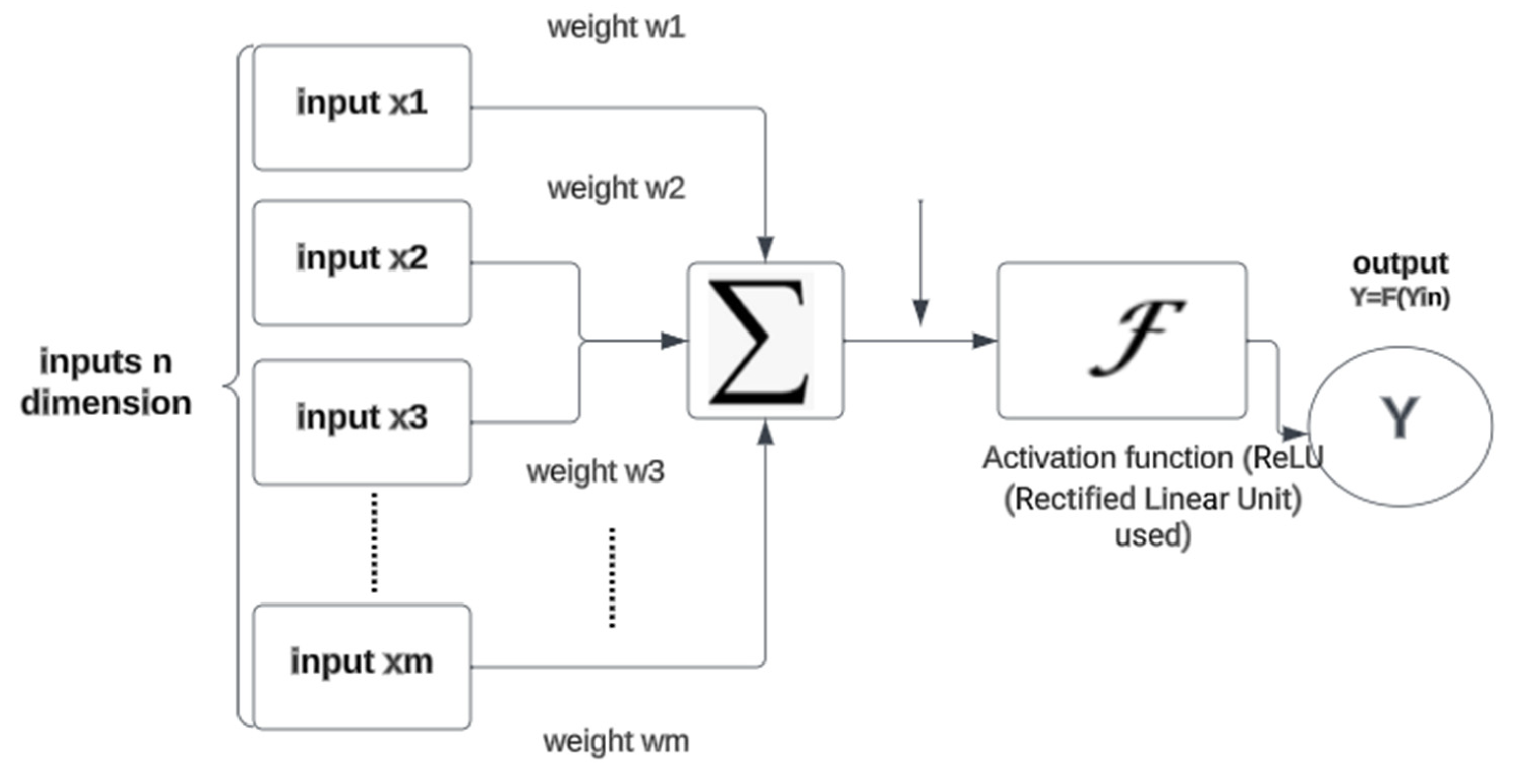
3.7.1. Artificial Neural Network (ANN)
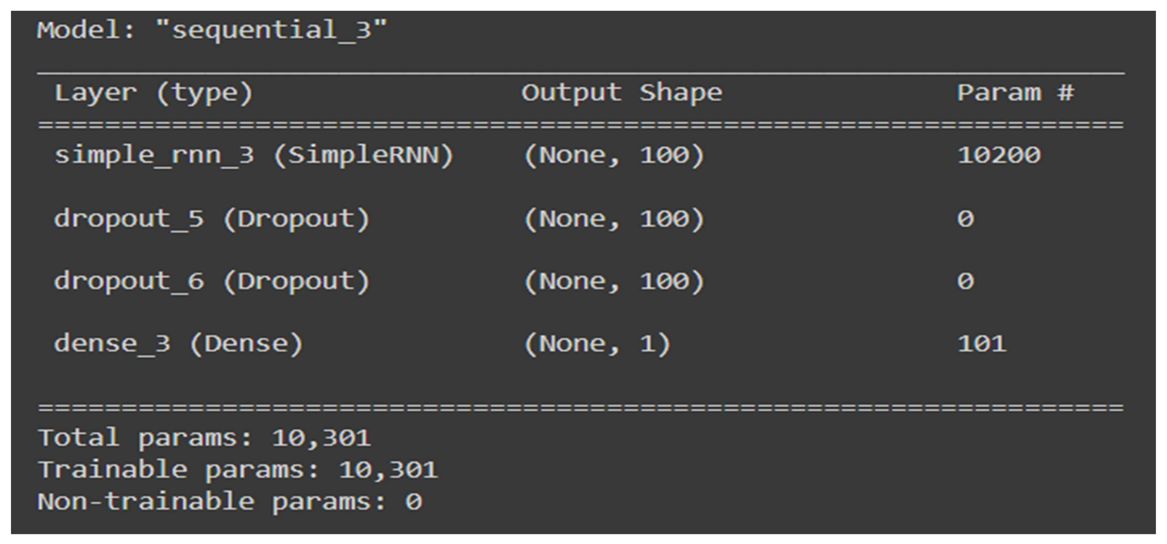
3.7.2. Recurrent Neural Network (RNN)
3.7.3. Long Short-Term Memory
3.8. Implementation Details
- The various machine learning models used in this study have been implemented using sk-learn.
- For deep learning models, tensorflow has been used.
- For optimising and finetuning of various hyperparameters, k-fold cross validation has been performed.
- In addition, earlystopping callback of tensorflow has been used.
- The models are trained for 30 epochs.
- The validation split is 20%.
- The ReLu activation function has been used along with Adam optimiser.
4. Criterion for Evaluating Models
4.1. RMSE (Root Mean Squared Error)
4.2. R-Squared (Coefficient of Determination)
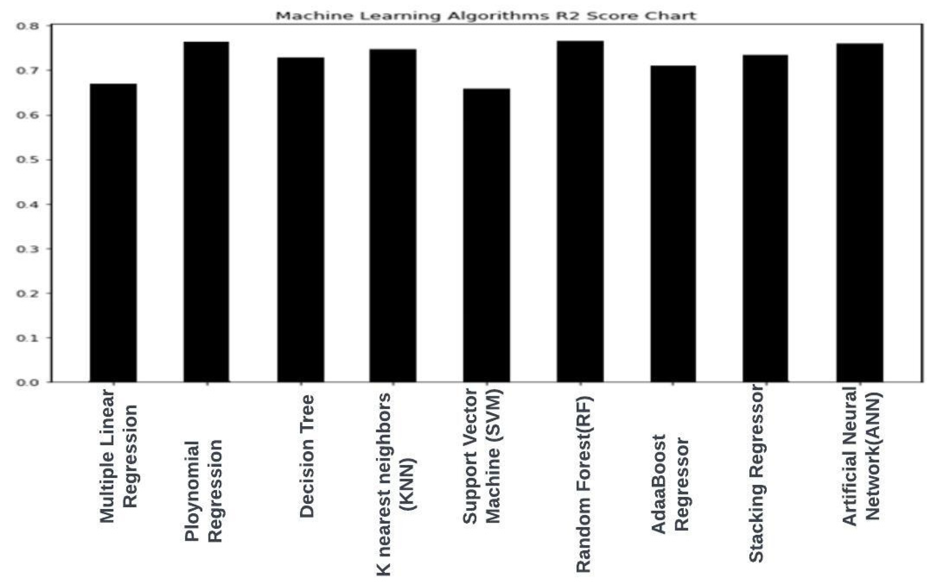
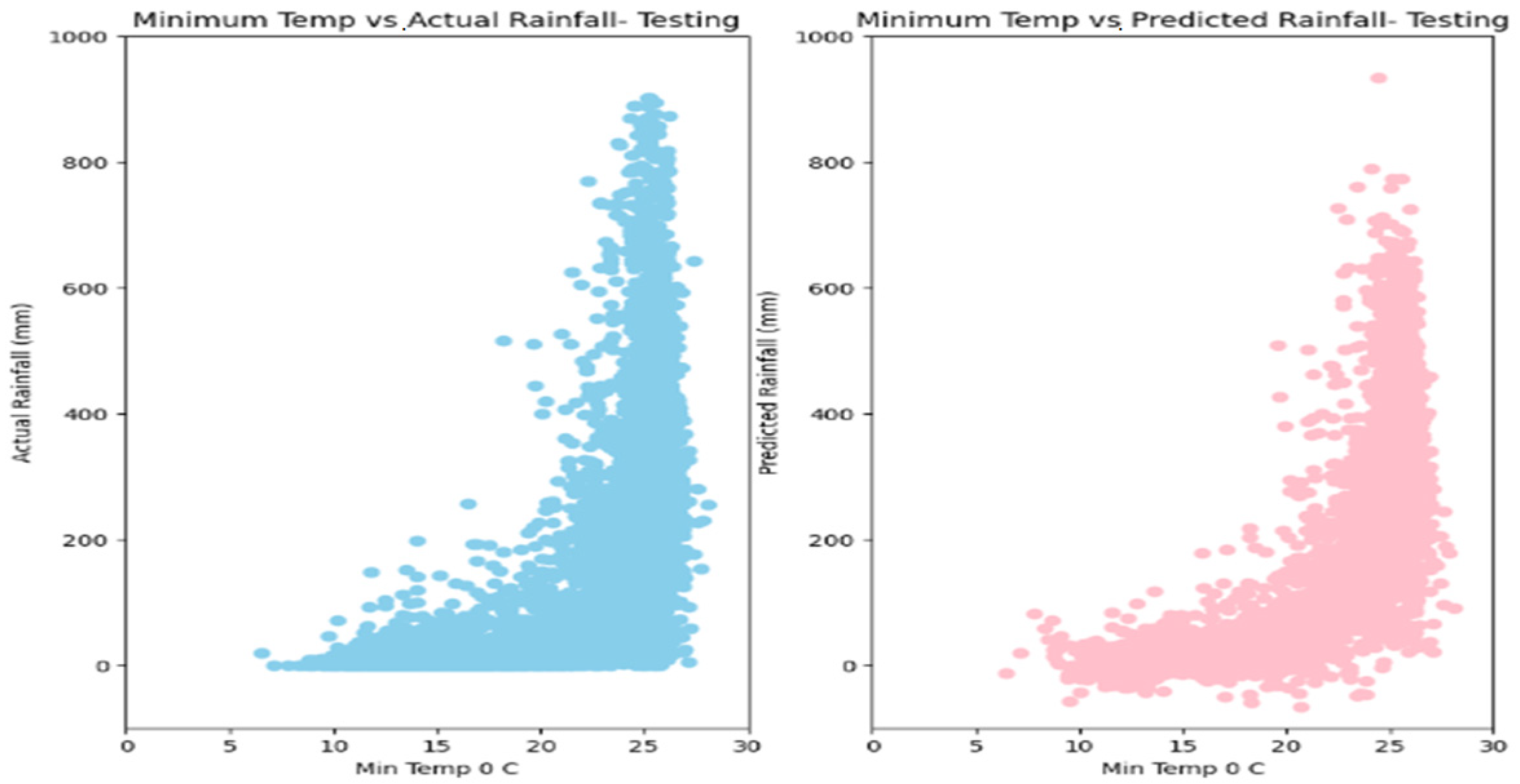
5. Results
6. Discussion
7. Conclusions and Future Work
Author Contributions
Funding
Data Availability Statement
Conflicts of Interest
References
- Syeed, M.M.A.; Farzana, M.; Namir, I.; Ishrar, I.; Nushra, M.H.; Rahman, T. Flood prediction using machine learning models. In Proceedings of the 2022 International Congress on Human-Computer Interaction, Optimization and Robotic Applications (HORA), Ankara, Turkey, 9–11 June 2022; IEEE: New York, NY, USA, 2022. [Google Scholar]
- Kumar, V.; Azamathulla, H.M.; Sharma, K.V.; Mehta, D.J.; Maharaj, K.T. The state of the art in deep learning applications, challenges, and future prospects: A comprehensive review of flood forecasting and management. Sustainability 2023, 15, 10543. [Google Scholar] [CrossRef]
- Gude, V.; Corns, S.; Long, S. Flood prediction and uncertainty estimation using deep learning. Water 2020, 12, 884. [Google Scholar] [CrossRef]
- Nguyen, D.T.; Chen, S.-T. Real-time probabilistic flood forecasting using multiple machine learning methods. Water 2020, 12, 787. [Google Scholar] [CrossRef]
- Furquim, G.; Pessin, G.; Faiçal, B.S.; Mendiondo, E.M.; Ueyama, J. Improving the accuracy of a flood forecasting model by means of machine learning and chaos theory: A case study involving a real wireless sensor network deployment in brazil. Neural Comput. Appl. 2016, 27, 1129–1141. [Google Scholar] [CrossRef]
- Talukdar, S.; Ghose, B.; Shahfahad; Salam, R.; Mahato, S.; Pham, Q.B.; Linh, N.T.T.; Costache, R.; Avand, M. Flood susceptibility modeling in Teesta River basin, Bangladesh using novel ensembles of bagging algorithms. Stoch. Environ. Res. Risk Assess. 2020, 34, 2277–2300. [Google Scholar] [CrossRef]
- Maspo, N.-A.; Bin Harun, A.N.; Goto, M.; Cheros, F.; Haron, N.A.; Nawi, M.N.M. Evaluation of Machine Learning approach in flood prediction scenarios and its input parameters: A systematic review. In IOP Conference Series: Earth and Environmental Science; IOP Publishing: Bristol, UK, 2020. [Google Scholar]
- Mitra, P.; Ray, R.; Chatterjee, R.; Basu, R.; Saha, P.; Raha, S.; Barman, R.; Patra, S.; Biswas, S.S.; Saha, S. Flood forecasting using Internet of things and artificial neural networks. In Proceedings of the 2016 IEEE 7th Annual Information Technology, Electronics and Mobile Communication Conference (IEMCON), Vancouver, BC, Canada, 13–15 October 2016; IEEE: New York, NY, USA, 2016. [Google Scholar]
- Noymanee, J.; Nikitin, N.O.; Kalyuzhnaya, A.V. Urban pluvial flood forecasting using open data with machine learning techniques in pattani basin. Procedia Comput. Sci. 2017, 119, 288–297. [Google Scholar] [CrossRef]
- Aswad, F.M.; Kareem, A.N.; Khudhur, A.M.; Khalaf, B.A.; Mostafa, S.A. Tree-based machine learning algorithms in the Internet of Things environment for multivariate flood status prediction. J. Intell. Syst. 2021, 31, 1–14. [Google Scholar] [CrossRef]
- Sankaranarayanan, S.; Prabhakar, M.; Satish, S.; Jain, P.; Ramprasad, A.; Krishnan, A. Flood prediction based on weather parameters using deep learning. J. Water Clim. Change 2020, 11, 1766–1783. [Google Scholar] [CrossRef]
- Wang, G.; Yang, J.; Hu, Y.; Li, J.; Yin, Z. Application of a novel artificial neural network model in flood forecasting. Environ. Monit. Assess. 2022, 194, 125. [Google Scholar] [CrossRef]
- Puttinaovarat, S.; Horkaew, P. Flood forecasting system based on integrated big and crowdsource data by using machine learning techniques. IEEE Access 2020, 8, 5885–5905. [Google Scholar] [CrossRef]
- Ria, N.J.; Ani, J.F.; Islam, M.; Masum, A.K.M. Standardization Of Rainfall Prediction In Bangladesh Using Machine Learning Approach. In Proceedings of the 2021 12th International Conference on Computing Communication and Networking Technologies (ICCCNT), Kharagpur, India, 6–8 July 2021; IEEE: New York, NY, USA, 2021. [Google Scholar]
- Osmani, S.A.; Kim, J.-S.; Jun, C.; Sumon, W.; Baik, J.; Lee, J. Prediction of monthly dry days with machine learning algorithms: A case study in Northern Bangladesh. Sci. Rep. 2022, 12, 19717. [Google Scholar] [CrossRef] [PubMed]
- Manandhar, A.; Fischer, A.; Bradley, D.J.; Salehin, M.; Islam, M.S.; Hope, R.; Clifton, D.A. Machine learning to evaluate impacts of flood protection in Bangladesh, 1983–2014. Water 2020, 12, 483. [Google Scholar] [CrossRef]
- Aydin, M.C.; Sevgi Birincioğlu, E. Flood risk analysis using gis-based analytical hierarchy process: A case study of Bitlis Province. Appl. Water Sci. 2022, 12, 122. [Google Scholar] [CrossRef]
- Msabi, M.M.; Makonyo, M. Flood susceptibility mapping using GIS and multi-criteria decision analysis: A case of Dodoma region, central Tanzania. Remote Sens. Appl. Soc. Environ. 2021, 21, 100445. [Google Scholar] [CrossRef]
- Shafizadeh-Moghadam, H.; Valavi, R.; Shahabi, H.; Chapi, K.; Shirzadi, A. Novel forecasting approaches using combination of machine learning and statistical models for flood susceptibility mapping. J. Environ. Manag. 2018, 217, 1–11. [Google Scholar] [CrossRef]
- Elmagzoub, M.; Syed, D.; Shaikh, A.; Islam, N.; Alghamdi, A.; Rizwan, S. A survey of swarm intelligence based load balancing techniques in cloud computing environment. Electronics 2021, 10, 2718. [Google Scholar] [CrossRef]
- Al Reshan, M.S.; Syed, D.; Islam, N.; Shaikh, A.; Hamdi, M.; Elmagzoub, M.A.; Muhammad, G.; Talpur, K.H. A Fast Converging and Globally Optimized Approach for Load Balancing in Cloud Computing. IEEE Access 2023, 11, 11390–11404. [Google Scholar] [CrossRef]
- Islam, N.; Raza, E.; Mohsin, S.; Ansari, A.; Shuja, R.; Syed, D. Forecasting on COVID-19 Data Using ARIMAX Model. In Data Science with Semantic Technologies; CRC Press: Boca Raton, FL, USA, 2023; pp. 95–113. [Google Scholar]
- Islam, N.; Khan, S.K.; Rehman, A.; Aftab, U.; Syed, D. Stock Prediction for ARGAAM Companies Dataset. KIET J. Comput. Inf. Sci. 2023, 6, 1–13. [Google Scholar] [CrossRef]
- Bui, D.T.; Pradhan, B.; Nampak, H.; Bui, Q.-T.; Tran, Q.-A.; Nguyen, Q.-P. Hybrid artificial intelligence approach based on neural fuzzy inference model and metaheuristic optimization for flood susceptibilitgy modeling in a high-frequency tropical cyclone area using GIS. J. Hydrol. 2016, 540, 317–330. [Google Scholar]
- Chatterjee, S.; Datta, B.; Sen, S.; Dey, N.; Debnath, N.C. Rainfall prediction using hybrid neural network approach. In Proceedings of the 2018 2nd International Conference on Recent Advances in Signal Processing, Telecommunications & Computing (SigTelCom), Ho Chi Minh, Vietnam, 29–31 January 2018; IEEE: New York, NY, USA, 2018. [Google Scholar]
- Islam, M.N.; van Amstel, A.; Ghosh, B.K.; Sarker, K.R. Climate Change and Living with Floods: An Empirical Case from the Saghata Union of Gaibandha District, Bangladesh. In Bangladesh II: Climate Change Impacts, Mitigation and Adaptation in Developing Countries; Springer: Cham, Switzerland, 2021; pp. 459–478. [Google Scholar]
- Luo, T.; Maddocks, A.; Iceland, C.; Ward, P.; Winsemius, H. World’s 15 Countries with the Most People Exposed to River Floods; World Resources Institute: Washington, DC, USA, 2015. [Google Scholar]
- Kumari, S.; Tripathy, K.K.; Kumbhar, V. Data Science and Analytics; Emerald Publishing Limited: Bingley, UK, 2020. [Google Scholar]
- Thirumalai, C.; Harsha, K.S.; Deepak, M.L.; Krishna, K.C. Heuristic prediction of rainfall using machine learning techniques. In Proceedings of the 2017 International Conference on Trends in Electronics and Informatics (ICEI), Tirunelveli, India, 11–12 May 2017; IEEE: New York, NY, USA, 2017. [Google Scholar]
- Adnan, R.; Zain, Z.M.; Ruslan, F.A. 5 hours flood prediction modeling using improved NNARX structure: Case study Kuala Lumpur. In Proceedings of the 2014 IEEE 4th International Conference on System Engineering and Technology (ICSET), Bandung, Indonesia, 24–25 November 2014; IEEE: New York, NY, USA, 2014. [Google Scholar]
- Mosavi, A.; Ozturk, P.; Chau, K.-W. Flood prediction using machine learning models: Literature review. Water 2018, 10, 1536. [Google Scholar] [CrossRef]
- Chen, C.; Jiang, J.; Liao, Z.; Zhou, Y.; Wang, H.; Pei, Q. A short-term flood prediction based on spatial deep learning network: A case study for Xi County, China. J. Hydrol. 2022, 607, 127535. [Google Scholar] [CrossRef]
- Motta, M.; de Castro Neto, M.; Sarmento, P. A mixed approach for urban flood prediction using Machine Learning and GIS. Int. J. Disaster Risk Reduct. 2021, 56, 102154. [Google Scholar] [CrossRef]
- Ghorpade, P.; Gadge, A.; Lende, A.; Chordiya, H.; Gosavi, G.; Mishra, A.; Hooli, B.; Ingle, Y.S.; Shaikh, N. Flood forecasting using machine learning: A review. In Proceedings of the 2021 8th International Conference on Smart Computing and Communications (ICSCC), Kerala, India, 1–3 July 2021; IEEE: New York, NY, USA, 2021. [Google Scholar]
- Adnan, M.S.G.; Siam, Z.S.; Kabir, I.; Kabir, Z.; Ahmed, M.R.; Hassan, Q.K.; Rahman, R.M.; Dewan, A. A novel framework for addressing uncertainties in machine learning-based geospatial approaches for flood prediction. J. Environ. Manag. 2023, 326, 116813. [Google Scholar] [CrossRef] [PubMed]
- Gauhar, N.; Das, S.; Moury, K.S. Prediction of flood in Bangladesh using K-nearest neighbors algorithm. In Proceedings of the 2021 2nd International Conference on Robotics, Electrical and Signal Processing Techniques (ICREST), Dhaka, Bangladesh, 5–7 January 2021; IEEE: New York, NY, USA, 2021. [Google Scholar]
- Han, S.; Coulibaly, P. Bayesian flood forecasting methods: A review. J. Hydrol. 2017, 551, 340–351. [Google Scholar] [CrossRef]
- Hamidul Haque, M.; Sadia, M.; Mustaq, M. Development of Flood Forecasting System for Someshwari-Kangsa Sub-watershed of Bangladesh-India Using Different Machine Learning Techniques. EGU General Assembly Conference Abstracts; EGU: Virtual, 2021. Available online: https://ui.adsabs.harvard.edu/abs/2021EGUGA..2315294H/abstract (accessed on 20 October 2023).
- Billah, M.; Adnan, N.; Akhond, M.R.; Ema, R.R.; Hossain, A.; Galib, S.M. Rainfall prediction system for Bangladesh using long short-term memory. Open Comput. Sci. 2022, 12, 323–331. [Google Scholar] [CrossRef]
- Yaseen, M.W.; Awais, M.; Riaz, K.; Rasheed, M.B.; Waqar, M.; Rasheed, S. Artificial Intelligence Based Flood Forecasting for River Hunza at Danyor Station in Pakistan. Arch. Hydro-Eng. Environ. Mech. 2022, 69, 59–77. [Google Scholar] [CrossRef]
- Parmar, A.; Mistree, K.; Sompura, M. Machine learning techniques for rainfall prediction: A review. In Proceedings of the International Conference on Innovations in Information Embedded and Communication Systems, Coimbatore, India, 17–18 March 2017. [Google Scholar]
- Khosravi, K.; Panahi, M.; Golkarian, A.; Keesstra, S.D.; Saco, P.M.; Bui, D.T.; Lee, S. Convolutional neural network approach for spatial prediction of flood hazard at national scale of Iran. J. Hydrol. 2020, 591, 125552. [Google Scholar] [CrossRef]
- Kovalchuk, S.V.; Krikunov, A.V.; Knyazkov, K.V.; Boukhanovsky, A.V. Classification issues within ensemble-based simulation: Application to surge floods forecasting. Stoch. Environ. Res. Risk Assess. 2017, 31, 1183–1197. [Google Scholar] [CrossRef]
- Nevo, S.; Morin, E.; Rosenthal, A.G.; Metzger, A.; Barshai, C.; Weitzner, D.; Voloshin, D.; Kratzert, F.; Elidan, G.; Dror, G.; et al. Flood forecasting with machine learning models in an operational framework. arXiv 2021, arXiv:2111.02780. [Google Scholar] [CrossRef]
- Khosravi, K.; Shahabi, H.; Pham, B.T.; Adamowski, J.; Shirzadi, A.; Pradhan, B.; Dou, J.; Ly, H.-B.; Gróf, G.; Ho, H.L.; et al. A comparative assessment of flood susceptibility modeling using multi-criteria decision-making analysis and machine learning methods. J. Hydrol. 2019, 573, 311–323. [Google Scholar] [CrossRef]
- El-Magd, S.A.A.; Pradhan, B.; Alamri, A. Machine learning algorithm for flash flood prediction mapping in Wadi El-Laqeita and surroundings, Central Eastern Desert, Egypt. Arab. J. Geosci. 2021, 14, 323. [Google Scholar] [CrossRef]
- Nayak, M.; Das, S.; Senapati, M.R. Improving Flood Prediction with Deep Learning Methods. J. Inst. Eng. Ser. B 2022, 103, 1189–1205. [Google Scholar] [CrossRef]
- Tayfur, G.; Singh, V.P.; Moramarco, T.; Barbetta, S. Flood hydrograph prediction using machine learning methods. Water 2018, 10, 968. [Google Scholar] [CrossRef]
- Sahoo, A.; Samantaray, S.; Ghose, D.K. Prediction of flood in Barak River using hybrid machine learning approaches: A case study. J. Geol. Soc. India 2021, 97, 186–198. [Google Scholar] [CrossRef]
- Qian, K.; Mohamed, A.; Claudel, C. Physics informed data driven model for flood prediction: Application of deep learning in prediction of urban flood development. arXiv 2019, arXiv:1908.10312. [Google Scholar]
- Miau, S.; Hung, W.-H. River flooding forecasting and anomaly detection based on deep learning. IEEE Access 2020, 8, 198384–198402. [Google Scholar] [CrossRef]
- Hossain, I.; Rasel, H.M.; Alam Imteaz, M.; Mekanik, F. Long-term seasonal rainfall forecasting using linear and non-linear modelling approaches: A case study for Western Australia. Meteorol. Atmos. Phys. 2020, 132, 131–141. [Google Scholar] [CrossRef]
- Ighile, E.H.; Shirakawa, H.; Tanikawa, H. Application of GIS and machine learning to predict flood areas in Nigeria. Sustainability 2022, 14, 5039. [Google Scholar] [CrossRef]
- Kunverji, K.; Shah, K.; Shah, N. A flood prediction system developed using various machine learning algorithms. In Proceedings of the 4th International Conference on Advances in Science & Technology (ICAST2021), Mumbai, India, 7 May 2021. [Google Scholar]
- Dodangeh, E.; Choubin, B.; Eigdir, A.N.; Nabipour, N.; Panahi, M.; Shamshirband, S.; Mosavi, A. Integrated machine learning methods with resampling algorithms for flood susceptibility prediction. Sci. Total Environ. 2020, 705, 135983. [Google Scholar] [CrossRef]
- Khairudin, N.M.; Mustapha, N.O.; Aris, T.N.; Zolkepli, M.A. A study to investigate the effect of different time-series scales towards flood forecasting using machine learning. J. Theor. Appl. Inform. Technol. 2021, 99, 5687–5699. [Google Scholar]
- Dtissibe, F.Y.; Ari, A.A.A.; Titouna, C.; Thiare, O.; Gueroui, A.M. Flood forecasting based on an artificial neural network scheme. Nat. Hazards 2020, 104, 1211–1237. [Google Scholar] [CrossRef]
- Sarasa-Cabezuelo, A. Prediction of rainfall in Australia using machine learning. Information 2022, 13, 163. [Google Scholar] [CrossRef]
- Liyew, C.M.; Melese, H.A. Machine learning techniques to predict daily rainfall amount. J. Big Data 2021, 8, 153. [Google Scholar] [CrossRef]
- Singh, P. Indian summer monsoon rainfall (ISMR) forecasting using time series data: A fuzzy-entropy-neuro based expert system. Geosci. Front. 2018, 9, 1243–1257. [Google Scholar] [CrossRef]
- Mishra, N.; Soni, H.K.; Sharma, S.; Upadhyay, A.K. Development and analysis of artificial neural network models for rainfall prediction by using time-series data. Int. J. Intell. Syst. Appl. 2018, 12, 16. [Google Scholar] [CrossRef]
- Chitwatkulsiri, D.; Miyamoto, H. Real-Time Urban Flood Forecasting Systems for Southeast Asia—A Review of Present Modelling and Its Future Prospects. Water 2023, 15, 178. [Google Scholar] [CrossRef]
- Kumar, V.; Sharma, K.V.; Caloiero, T.; Mehta, D.J.; Singh, K. Comprehensive overview of flood modeling approaches: A review of recent advances. Hydrology 2023, 10, 141. [Google Scholar] [CrossRef]
- Mosaffa, H.; Sadeghi, M.; Mallakpour, I.; Jahromi, M.N.; Pourghasemi, H.R. Application of Machine Learning Algorithms in Hydrology. In Computers in Earth and Environmental Sciences; Elsevier: Amsterdam, The Netherlands, 2022; pp. 585–591. [Google Scholar]
- Jehanzaib, M.; Ajmal, M.; Achite, M.; Kim, T.-W. Comprehensive review: Advancements in rainfall-runoff modelling for flood mitigation. Climate 2022, 10, 147. [Google Scholar] [CrossRef]
- Mistry, S.; Parekh, F. Flood Forecasting Using Artificial Neural Network. In IOP Conference Series: Earth and Environmental Science; IOP Publishing: Bristol, UK, 2022. [Google Scholar]
- Xu, Y.; Hu, C.; Wu, Q.; Jian, S.; Li, Z.; Chen, Y.; Zhang, G.; Zhang, Z.; Wang, S. Research on particle swarm optimization in LSTM neural networks for rainfall-runoff simulation. J. Hydrol. 2022, 608, 127553. [Google Scholar] [CrossRef]
- Cho, M.; Kim, C.; Jung, K.; Jung, H. Water level prediction model applying a long short-term memory (lstm)–gated recurrent unit (gru) method for flood prediction. Water 2022, 14, 2221. [Google Scholar] [CrossRef]
- Qadeer, K.; Rehman, W.U.; Sheri, A.M.; Park, I.; Kim, H.K.; Jeon, M. A long short-term memory (LSTM) network for hourly estimation of PM2.5 concentration in two cities of South Korea. Appl. Sci. 2020, 10, 3984. [Google Scholar] [CrossRef]
- Available online: https://www.kaggle.com/datasets/emonreza/65-years-of-weather-data-bangladesh-preprocessed (accessed on 20 October 2023).
- Wong, T.-T.; Yeh, P.-Y. Reliable accuracy estimates from k-fold cross validation. IEEE Trans. Knowl. Data Eng. 2019, 32, 1586–1594. [Google Scholar] [CrossRef]
- Rahman, M.; Chen, N.; Elbeltagi, A.; Islam, M.M.; Alam, M.; Pourghasemi, H.R.; Tao, W.; Zhang, J.; Shufeng, T.; Faiz, H.; et al. Application of stacking hybrid machine learning algorithms in delineating multi-type flooding in Bangladesh. J. Environ. Manag. 2021, 295, 113086. [Google Scholar] [CrossRef] [PubMed]


| Reference | Dataset | Model | Pros | Cons |
|---|---|---|---|---|
| [33] | Urban datasets from January 2013 and December 2018 | Machine Learning (RF) and GIS | A flood risk score was produced by combining the results of the random forest model and the Hot Spot research. | Hourly dataset; not a consistent forecast for the entire year. |
| [5] | Rainfall in April 2014 in Brazil | Chaos theory MLP, E-RNN | The outcomes demonstrate that the MLP outperforms the ERNN. | Not a consistent forecast for the entire year. |
| [4] | Yilan River basin and Taiwan 2012 to 2018 | (SVR), fuzzy inference model (FIM), (k-NN) | Statistical parameters are used to analyse time series data. | A less extensive training dataset, a smaller feature set, along with lower precision and recall. |
| [25] | Dumdum weather station | Hybrid neural framework | Selection of features: hybrid neural system. | Less precision just for a tiny area. |
| [29] | India’s annual rainfall is included in the data collection. | Linear regression | Assist farmers in making the best decision for harvesting a particular crop. | Based on only one characteristic, no experimental results were discovered. |
| [14] | Used the dataset of 2016 to 2019 of Bangladesh. | DT, KNN, LR, NB, RF | According to the results, random forest can make reliable forecasts for daily rainfall estimates. | Small dataset utilised for experiment. |
| [57] | Dataset reported of France. 2002 to 2018 events | Multiple linear regression (MLR) and non-linear modelling technique, (ANN) | The created model was tested extensively, and the results demonstrated the usefulness of forecasting. | Event-wise data analysis. |
| [60] | Data on Indian summer monsoon rainfall | Expert system based on fuzzy entropy | Statistical parameters are used to analyse time series data. | Less precision; covers a much smaller area. |
| [61] | The Indian Meteorological Institute in Pune collected data on North India’s monthly rainfall. | Artificial Neural Network (ANN) | Dataset with a long-time series. | Only 1- and 2-month forward forecast; minimal feature set. |
| Sr. No. | Attribute | Attributes Description | Type | Measurement |
|---|---|---|---|---|
| 1. | ‘Unnamed: 0’, | This is likely an index or identifier column for the dataset. | integer | serial no |
| 2. | ‘Station Names’ | The name of the city or station where the flood occurred | string | categorical |
| 3. | ‘Year’, | This column represents the year for which the weather data are recorded. | integer | numerical |
| 4. | ‘Month’, | The month of the recorded data. | integer | numerical |
| 5. | ‘Max Temp 0C’ | The maximum recorded temperature of a day. | float | degrees Celsius |
| 6. | ‘Min Temp 0C’ | The minimum temperature experienced on a specific day (degrees Celsius). | float | degrees Celsius |
| 7. | ‘Rainfall (mm)’, | The amount of rainfall recorded (millimetres). | float | millimetres |
| 8. | relative humidity | This column represents the relative humidity recorded for a specific month and year. | float | percentage |
| 9. | ‘Wind Speed’, | Wind speed in a particular direction at a given location and time | float | metres per second. |
| 10 | Cloud Coverage | This column represents the cloud coverage or cloudiness level recorded for a specific month and year. | float | percentage |
| 11 | ‘Bright Sunshine’ | This column contains the duration of bright sunshine recorded for a specific month and year. It represents when the sun is visible, or the sky is clear. | float | measured in hours |
| 12 | ‘Station Number’ | In meteorology and weather monitoring, a station number is a unique identification declared to an individual weather station or monitoring place. | integer | numerical identifier |
| 13 | ‘X_COR’, | This column could represent the X-coordinate or longitude values associated with the location of each weather station. | float | coordinates of the station |
| 14 | Y_COR | This column could represent the Y-coordinate or latitude values associated with the location of each weather station. | float | coordinates of the station |
| 15 | LATITUDE | The latitude of rainfall on specific locations and weather conditions. | float | latitude coordinate of the station. |
| 16 | LONGITUDE | The longitude of rainfall in specific locations and weather conditions. | float | longitude coordinate of the station. |
| 17 | ‘ALT’, | This column likely represents the altitude or elevation of each weather station. | num | metres |
| 18 | ‘Period’ | Rainfall measurements are gathered or recorded at a specific time step or period (year and month combined). | float | numeric |
| Unnam | YEAR | Month | Max Temp °C | Min Temp °C | Rainfall | Humidity | Wind Speed | Cloud Coverage | Bright Sunshine | Station Num | X_ COR | Y_ COR | LATITUDE | LONGITUDE | ALT | Period |
|---|---|---|---|---|---|---|---|---|---|---|---|---|---|---|---|---|
| 0.064153 | 0.025109 | 0.132680 | 0.256821 | 0.596625 | 1.000000 | 1.0000 | 0.316366 | 0.766821 | −0.673333 | 0.113804 | 0.167625 | −0.066154 | −0.105569 | 0.197805 | −0.009696 | 0.02536 |
| Parameter | Values |
|---|---|
| Framework | Sk-learn, tensorflow |
| Training, validation, testing | 60%, 20%, 20% |
| Number of epochs | 30 |
| Stopping criterion | Early stopping |
| Activation functions | ReLu |
| Optimiser | Adam |
| Validation criterion | 3-fold cross validation |
| Machine and Deep Learning Model | and RMSE | ||||
|---|---|---|---|---|---|
| S.No. | ML Model | Score Training | Score Testing | RMSE Score Training | RMSE Testing |
| 1. | Multiple Linear regression | 0.6643 | 0.6687 | 118.3231 | 118.279217 |
| 2. | Polynomial regression | 0.773177 | 0.7642164 | 99.12397 | 99.844 |
| 3. | Decision Tree mode | 0.75 | 0.72 | 101.195 | 123.27715 |
| 4. | k-nearest neighbours | 0.9992 | 0.74723 | 5.5840 | 103.31968 |
| 5. | Support vector machine | 0.654139 | 0.6583 | 120.108182 | 120.12110 |
| 6. | Random Forest | 0.96417 | 0.768234 | 38.656 | 99.5790 |
| 7. | AdaBoostRegressor | 0.7047 | 0.710915 | 110.9689 | 110.49437 |
| 8. | Stacking Regressor | 0.74631 | 0.738501 | 102.88535 | 106.1608 |
| 9. | Artificial Neural Network | 0.763247 | 0.75847 | 100.911 | 100.77041 |
| S. No | Model | Architecture | Parameters | Value |
|---|---|---|---|---|
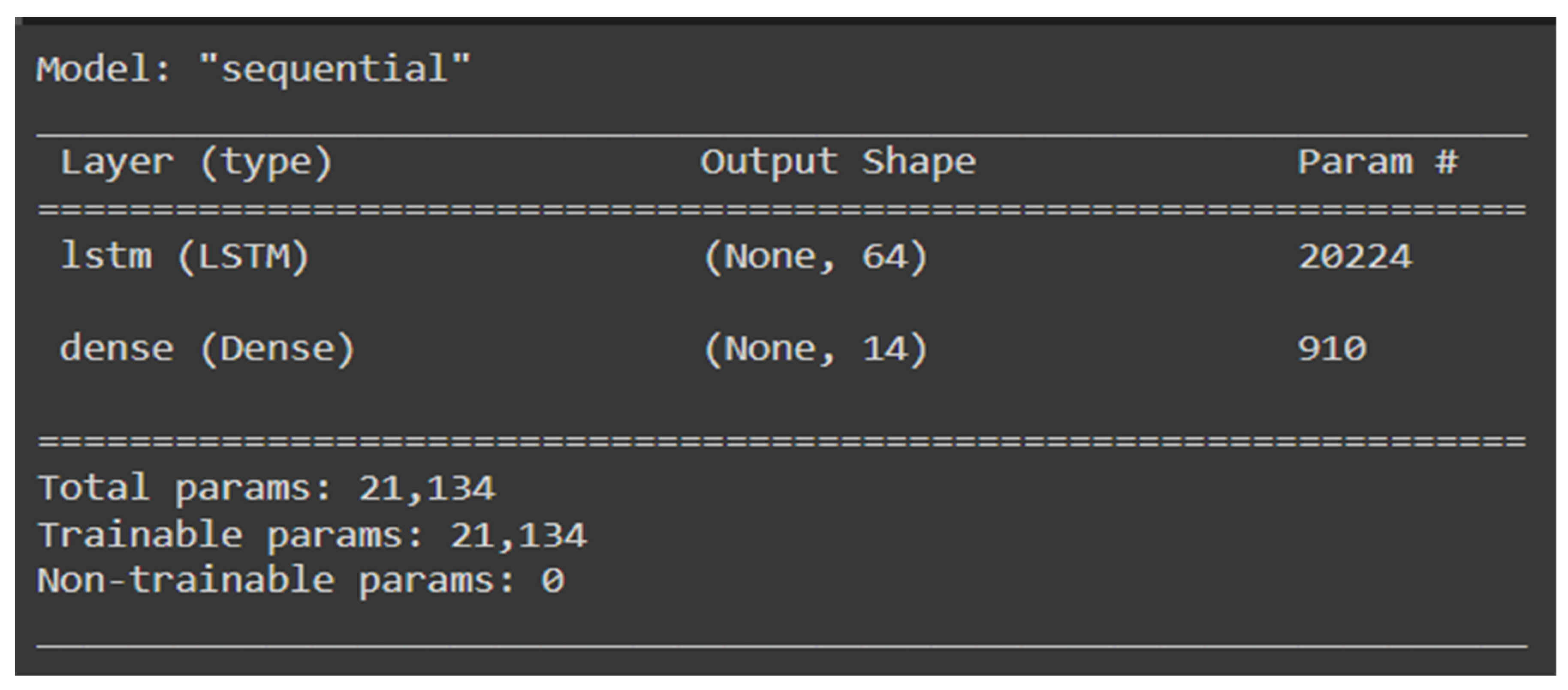
| 1. | LSTM In order to address and overcome the shortcomings of conventional RNNs, the LSTM approach was specifically developed for learning long-term dependencies. | Refer to Figure 23 | Loss | 0.0904 |
| RMSE | 0.3007 | |||
| Val_loss | 0.0906 | |||
| Testing set loss | 93,260.7188 | |||
| 2. | RNN The main feature of an RNN is its ability to maintain a hidden state or memory, which is revised at each time step and passed as input to the next, allowing the network to consider previous information while processing the current input. | Refer to Figure 24 | Loss | 126.5478 |
| mean_absolute_error: | 126.5478 | |||
| Val_loss | 124.1010 | |||
| Val_mean_absolute_error | 124.1010 |
Disclaimer/Publisher’s Note: The statements, opinions and data contained in all publications are solely those of the individual author(s) and contributor(s) and not of MDPI and/or the editor(s). MDPI and/or the editor(s) disclaim responsibility for any injury to people or property resulting from any ideas, methods, instructions or products referred to in the content. |
© 2023 by the authors. Licensee MDPI, Basel, Switzerland. This article is an open access article distributed under the terms and conditions of the Creative Commons Attribution (CC BY) license (https://creativecommons.org/licenses/by/4.0/).
Share and Cite
Rajab, A.; Farman, H.; Islam, N.; Syed, D.; Elmagzoub, M.A.; Shaikh, A.; Akram, M.; Alrizq, M. Flood Forecasting by Using Machine Learning: A Study Leveraging Historic Climatic Records of Bangladesh. Water 2023, 15, 3970. https://doi.org/10.3390/w15223970
Rajab A, Farman H, Islam N, Syed D, Elmagzoub MA, Shaikh A, Akram M, Alrizq M. Flood Forecasting by Using Machine Learning: A Study Leveraging Historic Climatic Records of Bangladesh. Water. 2023; 15(22):3970. https://doi.org/10.3390/w15223970
Chicago/Turabian StyleRajab, Adel, Hira Farman, Noman Islam, Darakhshan Syed, M. A. Elmagzoub, Asadullah Shaikh, Muhammad Akram, and Mesfer Alrizq. 2023. "Flood Forecasting by Using Machine Learning: A Study Leveraging Historic Climatic Records of Bangladesh" Water 15, no. 22: 3970. https://doi.org/10.3390/w15223970
APA StyleRajab, A., Farman, H., Islam, N., Syed, D., Elmagzoub, M. A., Shaikh, A., Akram, M., & Alrizq, M. (2023). Flood Forecasting by Using Machine Learning: A Study Leveraging Historic Climatic Records of Bangladesh. Water, 15(22), 3970. https://doi.org/10.3390/w15223970