Article

A Risk-Based Approach for the Analysis of Flood Impact in Villahermosa (Tabasco, Mexico)

by
Mackendy Ceragene
1,†,
Rosanna Bonasia
2,*,†,
Luis Cea
3 and
Maria de la O Cuevas-Cancino
4
1
Instituto Politécnico Nacional, Escuela Superior de Ingeniería y Arquitectura Unidad Zacatenco (ESIA), UZ, Miguel Bernard, S/N, Mexico City 07738, Mexico
2
School of Engineering and Sciences, Tecnologico de Monterrey, Carretera Lago de Guadalupe Km.3.5 Atizapán de Zaragoza Col. Margarita Maza de Juarez, Ciudad López Mateos 52926, Mexico
3
Environmental and Water Engineering Group, Department of Civil Engineering, Universidade da Coruña, 15001 A Coruña, Spain
4
School of Engineering and Sciences, Tecnologico de Monterrey, Av Carlos Lazo 100, Santa Fe, La Loma, Álvaro Obregón, Mexico City 01389, Mexico
*
Author to whom correspondence should be addressed.
These authors contributed equally to this work.
Water 2023, 15(22), 3969; https://doi.org/10.3390/w15223969
Submission received: 26 September 2023 / Revised: 30 October 2023 / Accepted: 2 November 2023 / Published: 15 November 2023

Abstract

:
Floods in Villahermosa are events that have occurred frequently over the centuries, due to the city’s location at the mouth of two of the most powerful rivers in Mexico. Flooding effects on residents have become increasingly damaging over the years as a consequence of the increase in frequency and intensity of extreme weather phenomena, in addition to poor land-use planning policies. The increase in population and consequent urban expansion are certainly causes of the problem, which are reflected in poor urban planning policy and in an almost absent perception of risk. In this work, we present a methodology for the construction of flood risk maps based on a hydraulic study, analysis of social vulnerability indexes, calculation of severity indexes and construction of hazard maps. The results of the hydraulic simulations show that relatively frequent rainfall causes floods of the order of 2 m, in agreement with annual observations conducted in Villahermosa. More extreme rainfall can lead to flooding greater than 4 m in marginalized areas of the city. The areas at greatest risk are sections close to the rivers that cross the city, and the estimated economic damage is greater than USD 14 million. Risk maps presented here constitute the first effort of an integrated study to couple flood analysis with the calculation of economic damage in the city of Villahermosa, and provide important tools to conscientize populations in their perception of risk, but also create the basis for a conscious urbanization policy.

1. Introduction

The state of Tabasco has been prone to flooding since historical times. In the 16th century, Spanish chroniclers, Vasco Rodríguez and Melchor Alfaro, wrote in their memoirs about Tabasco: “The land is flooded because of many rivers and because of the continuous winter there is” [1].
There are many causes responsible for the occurrence of floods in the state and in its capital Villahermosa. First of all, the state is located in the southeast region of Mexico, in a territory where two of the most powerful Mexican rivers converge, the Usumacinta and the Grijalva. Moreover, the region is characterized by the prevailing presence of clayey soil and is located above a semi-confined aquifer that prevents proper water infiltration, due to the propensity to saturation of the sub-surface layer of the soil. Apart from the natural causes that have led to floods since historical times (topography of the area, presence of large river networks, soil type in the alluvial plain), since the 1970s, the basins of these large rivers have experienced a process of intense deforestation which has substantially changed the land use from forest to agriculture, with a consequent radical runoff increase [2].
Another factor that increments the exposure of these lands to floods is the increase in frequency and intensity of tropical cyclones and other extreme weather phenomena, a fact that, from a climate change perspective, bears global effects [3,4]. During the last 20 years, Tabasco has witnessed extreme hydrometeorological events, which have caused losses of several USD million and deterioration of the region’s ecological system. In 1999, the conjunction of tropical waves, a tropical depression and cold fronts, caused the overflow of mountains rivers in the vicinity of Villahermosa. These floods prompted the construction of perimeter walls throughout the city and on the banks of the Carrizal and Grijalva rivers in the following year [5]. As a consequence of this event, in 2003, the Integral Flood Control Program (PICI) was developed as a proposed solution to the problem of systematic flooding in the capital city [6]. With this program, three hydraulic systems were planned to protect against the effects of extraordinary rainfall and confine the currents of the Samaria, Carrizal, de la Sierra and Grijalva rivers. However, the project was still in the feasibility study stage when the disastrous flood of 2007 occurred. This year, tropical cyclone Barbara hit the Grijalva river in June and the intense rainfall regime continued until the end of October accumulating 1423 mm of rain [5]. At the beginning of the weather event, the rain fell continuously for three days. Few people were warned that the dams in Chiapas would be opened, but without an official statement from the government. Twenty-four hours later, the water arrived with a very strong current and flooded 90% of the city in less that 12 h. In some places, it only took 20 min for the water to reach between 2.5 and 3 m depth. The entire city was flooded except for a 10-block radius close to where the cathedral is. People had been desperately trying to stop the downtown area from flooding for at least three days, piling sandbags along the Grijalva and Carrizal all day and all night. Unfortunately, it did not work. Once the water hit, people that were able to make it out of their homes were stuck on their roof tops, those who could not, drowned inside their homes. The level of the Grijalva river was above the ordinary maximum limit from October to November, and floods were also recorded in the Samaria and Usumacinta rivers. This caused the flooding of two-thirds of Villahermosa for almost 40 days. In April 2008, the PICI flood management scheme was reconsidered, for what would be the future Tabasco Comprehensive Water Program (PHIT) [7]. In 2010, two tropical cyclones led to an accumulated precipitation greater than the one originated in 2007 [5]. The large dams were pressured with significant water inflows, 12 of the 17 municipalities in the state of Tabasco were declared a disaster area [8] and all dam and river management protocols were reviewed and updated. In November 2020, a significant rainfall was recorded; flooding, landslides, and water discharge from the Peñitas hydroelectric dam left the region under water. Storms and subsequent flooding inundated 14% of the state, affecting 17 municipalities, damaging nearly 900 communities, with 10,000 evacuees, and flooding thousands of acres of crops across the state. Floods also damaged 2000 km of roads, affected drainage systems and major urban infrastructure, which suffered damages between USD 37 and 93 million [9].
From the chronicles of these events, it emerges that, for the state of Tabasco, the prevention policy aimed at minimizing the damage caused by floods is ineffective. To carry out a fruitful flood risk management, a long-term assessment of both the probability of occurrence of the phenomenon and its impact is necessary. Risk maps make it possible to obtain a complete view not only of the flood frequency and magnitude, but also of its consequences, providing precise information regarding the damage that a given event can cause. This derives from the risk definition that results from the product of the event occurrence probability (hazard), by the material consequences deriving from it [10]. The strong spatio-temporal component of risk maps makes them a fundamental tool for prevention policy and correct territorial planning. Moreover, risk maps are pivotal for risk communication, as they provide information that promotes public awareness about the actions that can be taken to minimize damage [11,12]. In the last 30 years, several governments around the world have changed the paradigm of traditional strategies for the prevention of flood damage that first was based on mainly structural solutions aimed at protecting flood-prone regions, following the effects of recent events. Many countries, nowadays, have recognized the importance of tackling the problem with a risk-based approach [13,14]. From the study by de Moel et al. [13], it is possible to examine an exhaustive review of the projects and solutions undertaken in Europe to deal with flooding. The United States Federal Emergency Management Agency (FEMA) introduced the National Flood Insurance Program (NFIP) in 2002 [15] with the objective of acquiring insurance as a safeguard against flood-related losses, in return for adhering to state floodplain management regulations. In Norway, Sweden, Finland, and the United Kingdom, flood hazard maps and risk information serve both as tools for spatial planning and as informative resources for decision-makers [16]. The perception of risk by populations is a factor that has an enormous influence on the analysis of vulnerability and consequently of the risk itself. In the work of Burningham et al. [17], it is observed that the incorrect perception of risk in many cases is the result of a risk assessment based on an underestimation of the real impact that a flood can have, hence the urgency of urging populations to participate in awareness and education plans. With the aim of increasing risk awareness, experiments have recently been conducted to demonstrate the potential advantages of virtual and augmented reality as an educational tool in environmental sciences and to provide new tools for communicating important data in planning and decision-making operations [18].
In Mexico, guidelines for the construction of risk maps and quantitative determination of damage caused by floods were established in 2014 [19]. These guidelines produced the National Atlas of Flood Risk [20] that, however, at present, only provides information on flood rates and historical flooding. It is evident, therefore, that an approach based on long-term flood risk forecasting is still absent in decision-making policies, spatial planning and implementation of actions for damage analysis and minimization. The development and use of risk maps would help to foster collaboration between vulnerable communities and local decision makers, implementing what is termed a Participatory Approach [21,22]. Furthermore, risk maps encourage the ability to understand, at the community level, one’s own vulnerability, implement shared strategies and activities, to manage flood risk without waiting for the intervention of external entities [23].
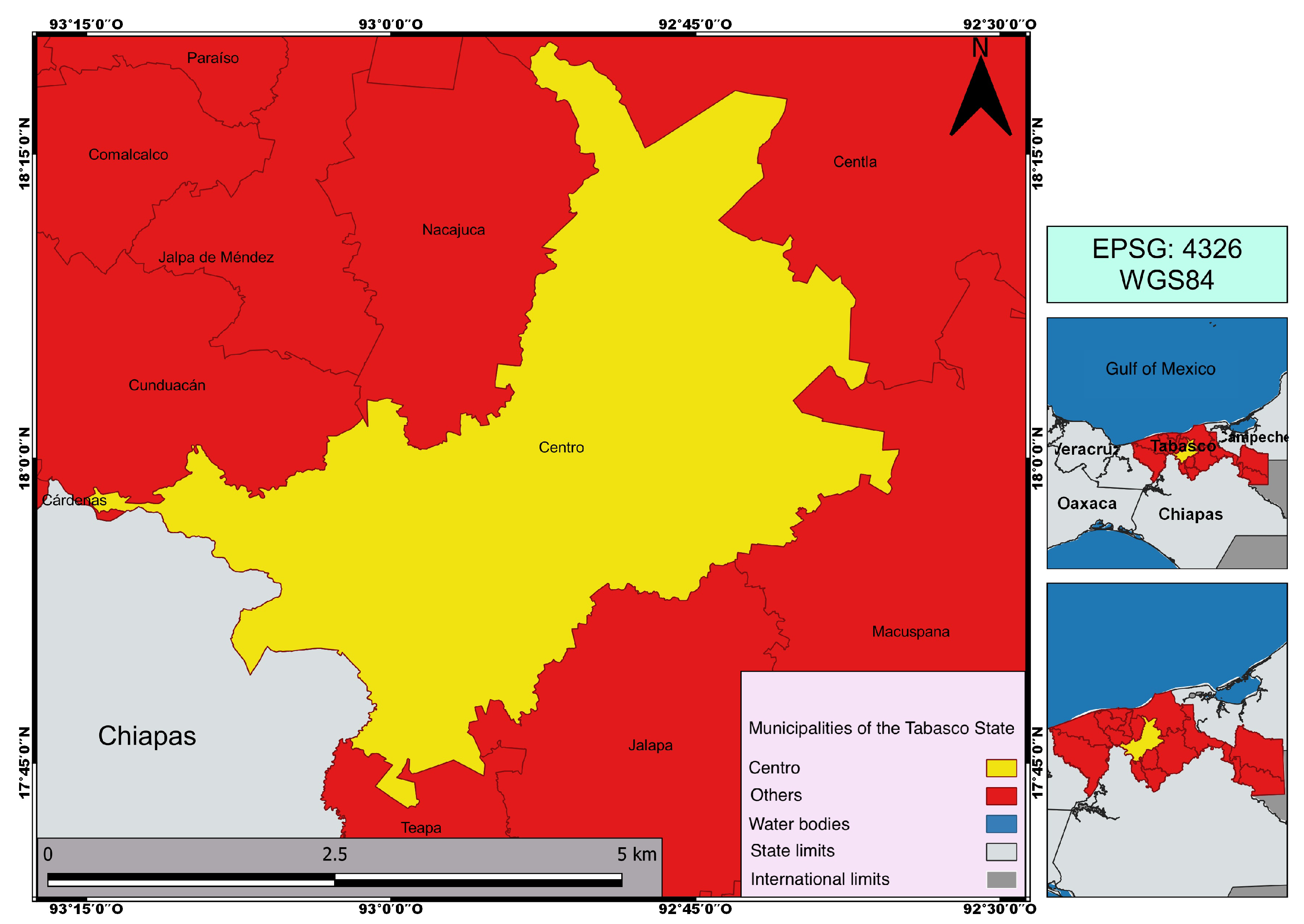
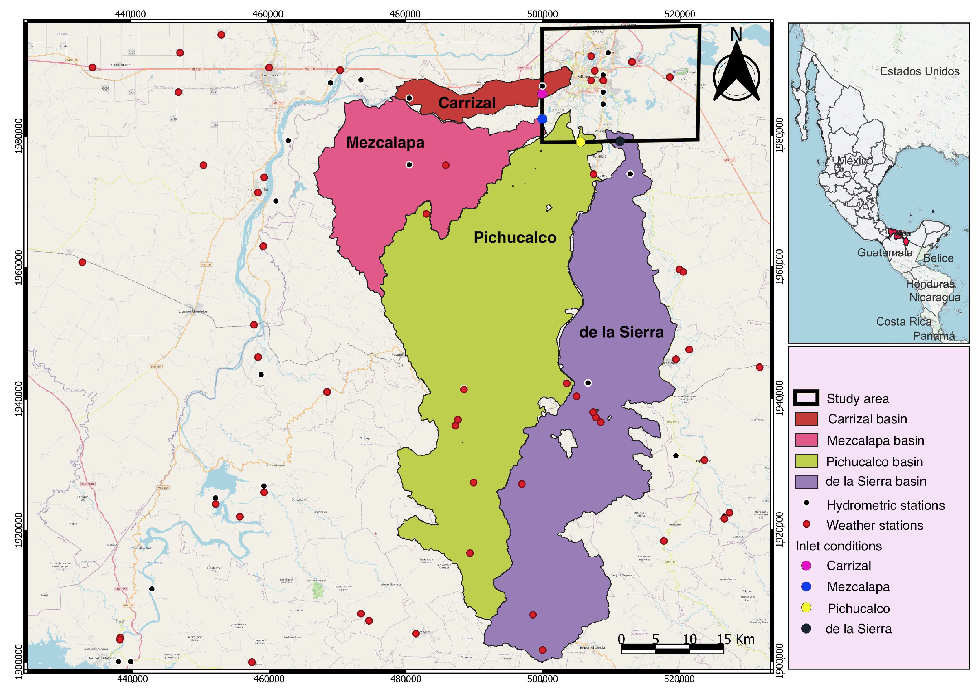
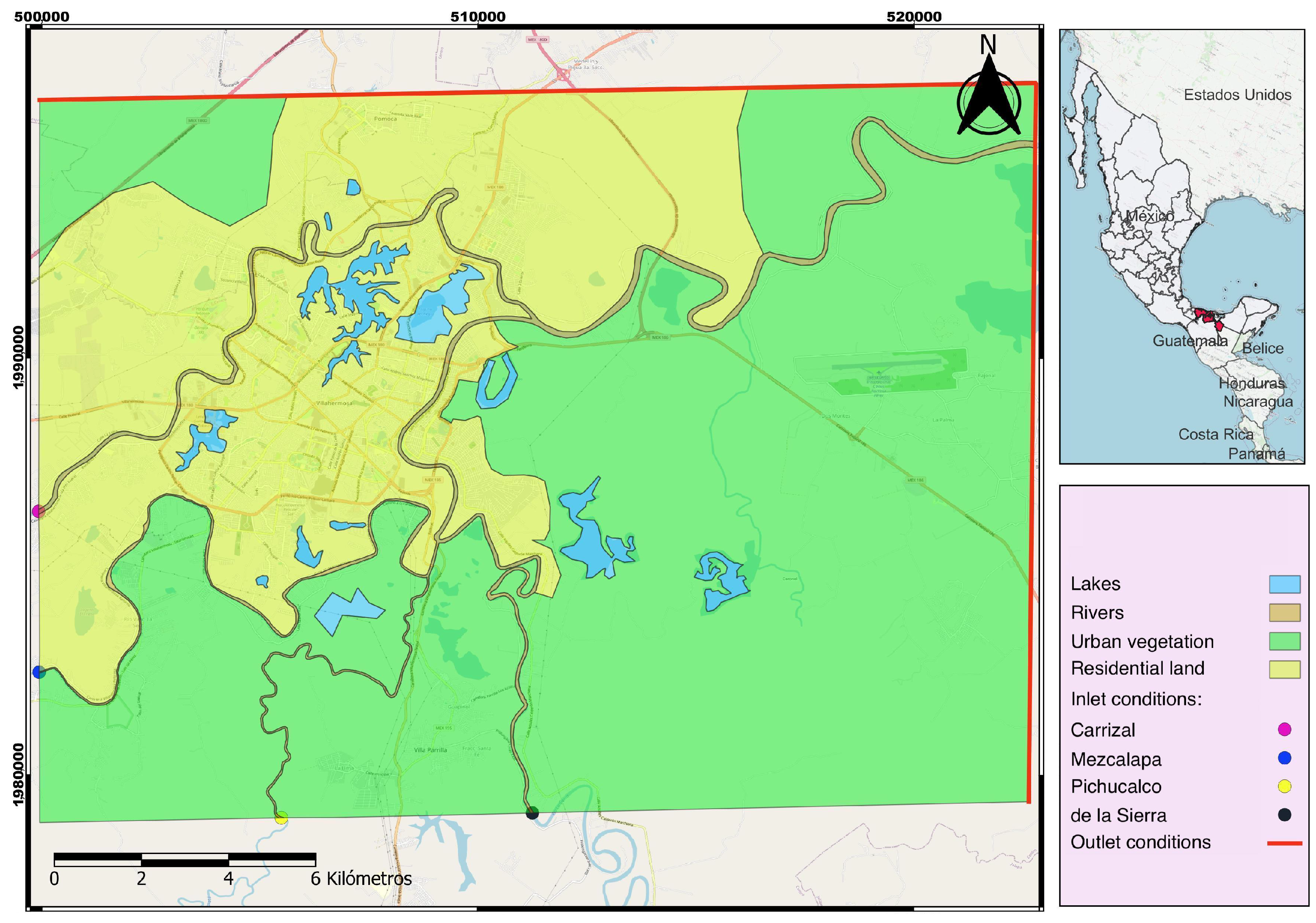
In this work, first risk maps for Villahermosa, one of the most flood-affected cities in Mexico, have been constructed. The methodology applied follows the previously mentioned guidelines of the National Water Commission, to additionally obtain a preliminary estimate of the expected economic damage in the face of different flood scenarios. First of all, a hydrological study was conducted to calculate design flows that intervene on Villahemosa (Section 2.1). Obtained design hydrographs, corresponding to different return periods, were used as input to the hydraulic simulations of flood scenarios, described in Section 2.2. Section 2.3 shows the methodology applied for the construction of vulnerability maps. In this part, social vulnerability indexes are calculated in accordance with the concepts expressed by various authors, according to which economic variables alone are not sufficient to describe the condition of vulnerability of a region [24,25]. Here, in the definition of social vulnerability indexes, the factors that influence the interaction between the community and exposure to floods are considered: socio-economic profile, employment, education and housing composition [26,27]. Subsequently, hazard maps were constructed based on the severity index calculation, to determine the impact on residential structures (Section 2.4). Finally, from a Gis-based intersection of hazard maps with the vulnerability map, risk maps were built as described in Section 2.5. From the results shown in Section 3, it can be seen that most affected areas are located in the south and southeast of the city, for low return periods, while as the return period increases, northern sectors are also at risk. Although most of the affected areas of the city show a medium risk, the economic damage expected annually from relatively frequent rainfall would exceed USD 14 million.

2. Materials and Methods

2.1. Design Flows Calculation

The Tabasco state is located within the Gulf of Mexico Coastal Plain, characterized by few reliefs and for more than 95% of its surface below 100 m above sea level. The region is characterized by a predominantly hot humid climate, with very frequent rainfall throughout the year with intensification from June to October [28]. According to data from the National Institute of Statistics and Geography (INEGI) [29], the runoff coefficient in the catchment area of the Grijalva and Usumacinta rivers ranges between 20 and 30% of all Mexican territory. The capital, Villahermosa, is located in the Centro municipality (Figure 1), within the Grijalva-Usumacinta hydrological region.
The hydrological study starts from the reconstruction of the temporal and spatial distribution of rainfall, through the transformation of punctual rainfall into rainfall–runoff relationships. Based on the work of Areu-Rangel et al. [30], in this study, of the 83 basins that compose the Grijalva-Usumacinta hydrological zone, four basins were considered, directly responsible for floods in the state capital: the Carrizal, Viejo Mezcalapa, Pichucalco and de la Sierra rivers. Figure 2 shows the sub-basins delimited from the outlet point of each river, the climatological and hydrometric stations available in the area, as well as the delimitation of the study area for the analysis of flood scenarios.
Table 1 shows the morphological characteristics of the sub-basins, together with the values of the concentration time, delay time, peak time and base time.
Regarding hydrometric stations selection, as can be seen in Figure 2, there are only a few stations in the study area, most of which have only a few years of records. For this reason, 83 climatological stations present in a radius of 80 km from the center of the Pichucalco river basin (the largest of the selected basins), were considered. For each station, data from daily precipitation records (every 24 h) were extracted from the Mexican Surface Climatic Stations Database (CLICOM System: Climate Computing [31]). Daily precipitation data were converted into maximum monthly rainfall and subsequently into maximum annual rainfall. The precipitation data obtained were compared with data provided by the National Meteorological Service, managed by the National Water Commission (CONAGUA [32]), to discard values affected by errors. Based on this comparison, the number of usable stations was reduced to 30. For each sub-basin, a set of stations was extracted and a single record of maximum annual rainfall values was built. Data from each single sub-basin record were analyzed with independence Anderson’s method [33]) and homogeneity (Helmert, Student t test and Cramer’s methods [34]) tests. Subsequently, a frequency analysis was performed on a total number of annual precipitation maximum records, corresponding to 72 years, using the Gumbel and Generalized Extreme Value (GEV) probability distribution functions since those are the recommended to fit an extreme value sample obtained with the annual maxima method. The statistical parameters corresponding to the maximum annual precipitation are as follows: mean = 161 mm and Standard Deviation = 53 mm. Table 2 shows the standard errors corresponding to the Carrizal river sub-basin, obtained for both distribution functions. It should be noted that the standard errors shown in Table 2 are only valid in the area or probability of the recorded data, but not outside, and therefore, they are not a measure of the extrapolation error to higher return periods. The independence and homogeneity tests on the extreme value sample, as well as the fit of the Gumbel and GEV parameters, were done with the software AFA v.1.2. for frequency analysis [35].
The Gumbel distribution function was found to be, in this case, the one with the smallest standard error using the maximum likelihood method, and was considered as the best distribution function to extrapolate the precipitation data at different return periods. The maximum annual precipitation values, with a duration of 24 h, extrapolated with the Gumbel function, were converted into short-term precipitations, up to 240 min, using the Bell’s adjusted formula [36,37]:
P t T = ( 0.54 t 0.25 0.50 ) P T 60 ,
where P t T is the rainfall in mm, for a return period T and a t-minutes duration, P t 60 is the precipitation in mm associated to a T-years return period and a duration of 60 minutes, t is the rainfall duration in minutes.
Excess rainfall was calculated by applying the Soil Conservation Service’ curve number method [38], based on total rainfall and land use:
P e = h p 508 N + 5.08 2 h p + 2032 N 20.32 ,
where P e is the excess precipitation in cm, h p is the accumulated annual precipitation in cm, extrapolated from the Gumbel distribution function, and N is the curve number. An average curve number was calculated for each sub-basin, starting from the soil use and type recongnized in the area. Figure 3 show the curve number distribution maps for the Carrizal and Viejo Mezcalapa sub-basins; Figure 4 correspond to the Pichucalco and de la Sierra sub-basins. The calculated values of the average curve numbers are also indicated within the figures.
Design flows were calculated as:
Q d = 0.208 P e A c t p ,
where Q d is the design flow corresponding to a given return period in m 3 /s, P e is the excess precipitation in mm, t p is the peak time in hours and A c is the basin’ area in km2. Table 3 shows the extrapolated 24-h annual maximum precipitation values ( h p ), excess precipitation ( P e ) and design flow values ( Q d ), calculated for different return periods, in each sub-basin.
Figure 5 and Figure 6 show the design hydrographs obtained for the four sub-basins, which will be used as hydrological input for the flood scenarios simulations.

2.2. Hydraulic Simulations of Flood Scenarios

Flood scenarios were simulated using Iber software. The characteristics of the model as well as its applicability and numerous validations can be consulted in Bladé et al. [39], Fraga et al. [40] and Cea and Bladé [41], among others. The software allows the possibility of working with three calculation modules, exploiting structured and unstructured finite volume meshes. For the specific purpose of this study, the hydrodynamic module was employed to compute flood scenarios. This module focuses on solving the depth-averaged shallow water equations, known as the two-dimensional Saint Venant equations, assuming a hydrostatic pressure distribution and relatively uniform velocity distribution across depths, where the only parameter requiring calibration is the Manning coefficient.
Figure 7 shows the location of the study area. The computation domain is characterized by the delimitation of two main land uses: residential and urban vegetation. The map also shows water bodies, rivers that cross the city, and the location of the inlet and outlet points for the definition of the boundary hydraulic conditions.
The calculation domain covers an area of 394,062 km 2 . For the geometry construction, a digital elevation model extracted from the database of INEGI [42], with a resolution of 15 m, was used. A preliminary model calibration analysis was performed with the aim of combining the appropriate parameters of roughness, mesh size, total simulation time and time step, in order to reach a steady flow. Selected conditions for optimal simulations, in terms of computational cost and flow stability, are shown in Table 4.
The computational domain was geometrically discretized with a non-structured triangular mesh composed of 220,802 elements. The boundary conditions of the inlets and outlets were assigned in the four entry points of the Carrizal, Mezcalapa, Pichucalco and de la Sierra rivers, shown as coloured dots in Figure 7. Inlet boundary conditions correspond to the hydrographs calculated for different return periods. Results of hydraulic simulations are maximum water depths and maximum water velocities.

2.3. Construction of Vulnerability Maps

Vulnerability maps were built using social vulnerability indexes (SVI), according to the methodology proposed by the Mexican Institute of Water Technology [43]. On the basis of the information present in the national statistics by INEGI and the National Population Council (CONAPO), 15 indicators are selected that can be grouped into 5 broad categories, which describe the development capacity of a community: (i) employment and income, (ii) education, (iii) health, (iv) housing, and (v) population. Table 5 shows the indicators that reflect the vulnerability of the population to flood related risks.
Sources used to generate the database for the calculation of the percentage coverage of each indicator are as follows: Population and Housing Census 2020 [44] and Marginalization Index 2020 [45].
For the calculation of the SVI, the following methodology was followed:
  • Starting from the coverage percentage of each indicator, their highest and lowest values, as well as the interval between them were recorded.
  • This interval was divided between the number of categories according to which the vulnerability condition is determined (in this case five) and the value defining the extent of each vulnerability level was calculated.
  • The extreme values of the vulnerability are constructed: Very High, or Very Low. In cases where the variable indicates a shortage of the population (for example the lack of drainage systems), the value encountered corresponds to a greater vulnerability. While, in cases where the variable indicates a satisfaction for the population (for example the level of education), the value found is equivalent to a lower vulnerability. To construct the intervals of the intermediate vulnerability conditions (ranges considered as Low, Medium and High), the procedure is as follows: one thousandth is added to the highest value of the immediately preceding vulnerability condition (0.001) and the result constitutes the lower limit of the vulnerability in construction. Subsequently, the interval is added to said value and thus the upper limit of this condition is obtained; this procedure is repeated to obtain the next range.
  • Once the indicators have been classified, they are assigned a rating ranging from 1.00 (Very High Vulnerability) to 0.20 (Very Low Vulnerability).
This procedure was applied to Villahermosa by dividing the city into districts with the same geostatistical characteristics (five districts that for sake of simplicity are enumerated from 1 to 5). Table 6 shows the values calculated for the different indicators in the five areas, while the values of the social vulnerability indexes obtained are indicated in Table 7.

2.4. Calculation of Severity Indexes and Construction of Hazard Maps

A severity analysis was conducted for the construction of hazard maps. The methodology applied in this work follows the study carried out by the Government of New South Wales, Australia, in 2007, on the risk of flooding in Dorrigo, crossed by the Bielsdown River [46]. In this study, flow velocity is correlated against hydraulic flood depth to determine the resistance of house’s walls, and then define hazard indexes. This method is considered within the guidelines for the construction of flood hazard maps in Mexico [19]. The aforementioned study establishes hazard indexes classified by color (Red—Very High; Orange—High; Yellow—Medium; Blue—Low; Green—Very Low). This rating, along with the corresponding water speed and depth thresholds, are shown in Table 8. Hazard maps have been constructed using results of maximum water velocities and depths, obtained from flood scenario simulations.

2.5. Construction of Risk Maps

Risk maps were obtained by intersecting flood hazard maps with vulnerability maps on a Gis bases, using the QGis program. The quantification of the potential economic damage caused by flooding was achieved by calculating a risk index. Following the guidelines for the construction of risk maps, established by CENAPRED in 2006 [47], the risk index used in this work is defined as:
I R j = R j C M A X ,
where R j represents the risk and C M A X is the value of the highest exposed property within the locality. R j is defined by the following expression:
R j = i = 1 m C j P ( i ) · V i ( Y i ) ,
where the subindex i refers to each of the return periods analyzed, and j refers to the houses and properties exposed. P ( i ) and V i ( Y i ) are the hazard and vulnerability functions, respectively. Based on the risk index value obtained from Equation (4), CENAPRED classifies the flood risk as shown in Table 9.
The possible economic damage caused by floods was calculated using the potential damage curves relating the water depth to the costs that could be incurred as a result of the damage, calculated by Baró-Suárez et al. [48]. In this work, the unit damages in terms of minimum wage were calculated for each house affected. Equations describing the potential damage curves are shown in Table 10.

3. Results

3.1. Flood Maps

Figure 8 and Figure 9 show the results of the hydraulic simulations in terms of maximum water depths in correspondence with four return periods (10, 50, 100 and 500 years). Return periods of less than 10 years have been discarded because they do not produce a significant impact on the study area.
The overview of the maps shows that in general, the area of the city most likely to be flooded is the southern one, which is mostly cultivated land. The urban areas affected are limited to a small portion of the city located to the southeast. For particularly frequent precipitation events (10-year return period), the maximum flood depths can exceed 2 m in rural areas south-east of the city. As the return period increases, flooding is also observed in the northwest, with maxima of the order of 1.50 m, while the southern portion of the city is affected by floods ranging from 1.50 m to maxima greater than 4 m.
Figure 10 shows hydraulic simulations results for maximum water velocities. On the map, we show the results for the lower and higher return period.
From the maps we can observe that the maximum flow velocity fluctuates around 2.60 m/s.

3.2. Vulnerability Maps

Figure 11 shows the social vulnerability map obtained for Villahermosa.
The map shows the degree of social vulnerability to which each district of the city is exposed. Most neighborhoods in Villahermosa fall into a low- to very-low classification of social vulnerability. There are few neighbourhoods with medium vulnerability, while there are only two neighbourhoods with high vulnerability.

3.3. Hazard Maps

Figure 12 and Figure 13 show the hazard maps, for the four return periods, obtained by relating water flow velocity with water depth in order to define the flood impact on houses in terms of a hazard index.
In all the maps, it can be observed that the districts of the city most affected by floods that present a high hazard are located close to the rivers that cross the city, in the external part of the central urban area, with a greater concentration in the south. The city center does not suffer from flooding due to its higher topography, and consequently does not present a hazard.

3.4. Risk Maps and Potential Economic Damage

Figure 14 and Figure 15 represent flood risk maps for Villahermosa.
In general, maps do not show districts of the city with a high risk of flooding, even in low-probability flood scenarios (high return periods). Most of the areas that have shown susceptibility to flooding are at medium risk, while very few are at low risk. On the basis of risk maps, the potential economic damage determined by the different flood scenarios was calculated for the districts at risk of flooding. The quantification of the damage was done considering the equations of Table 10 and the social vulnerability indexes of Figure 11. For the damage cost calculation of properties exposed to flood risk, the value of the daily minimum wage was taken into consideration that corresponds to MXN 207.44, according to the 2022 table of the National Minimum Wage Commission [49].
As an example of the result of the annual economic damage calculation in Villahermosa, the value of the expected damage as a result of a flood caused by the scenario with a 10-year return period is shown in Table 11. The calculation was made on the basis of affected inhabitants number, housing units, floodable surface area, number of people with minimum wages, economic values of exposed properties, risk index and risk classification.
Results show that under a relatively frequent flood scenario (10-year return period), 13.86 km 2 of the city of Villahermosa could be at risk of flooding. This area corresponds to 65.32% of the total floodable surface of the study area, where more than 33,000 people would be affected with a total economic damage of more than MXN 250 million.

4. Discussion

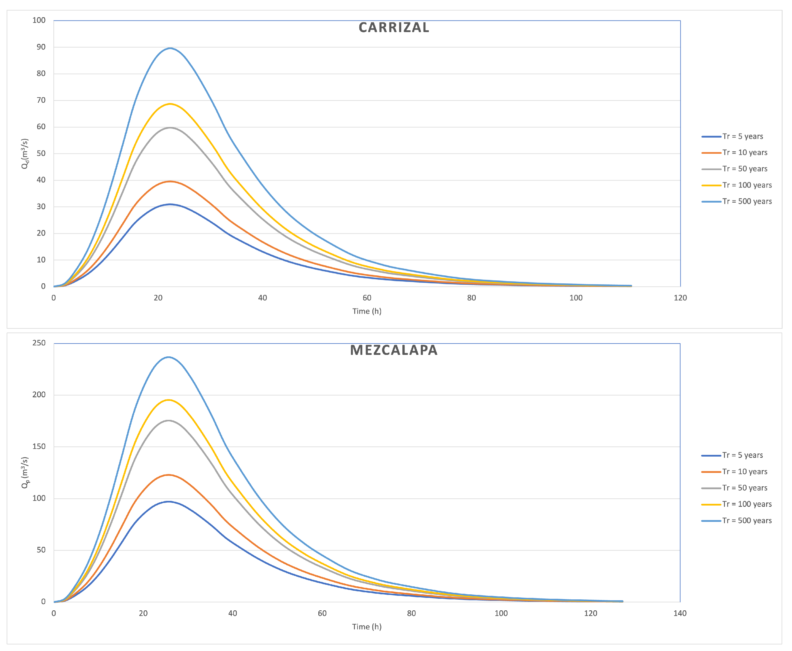
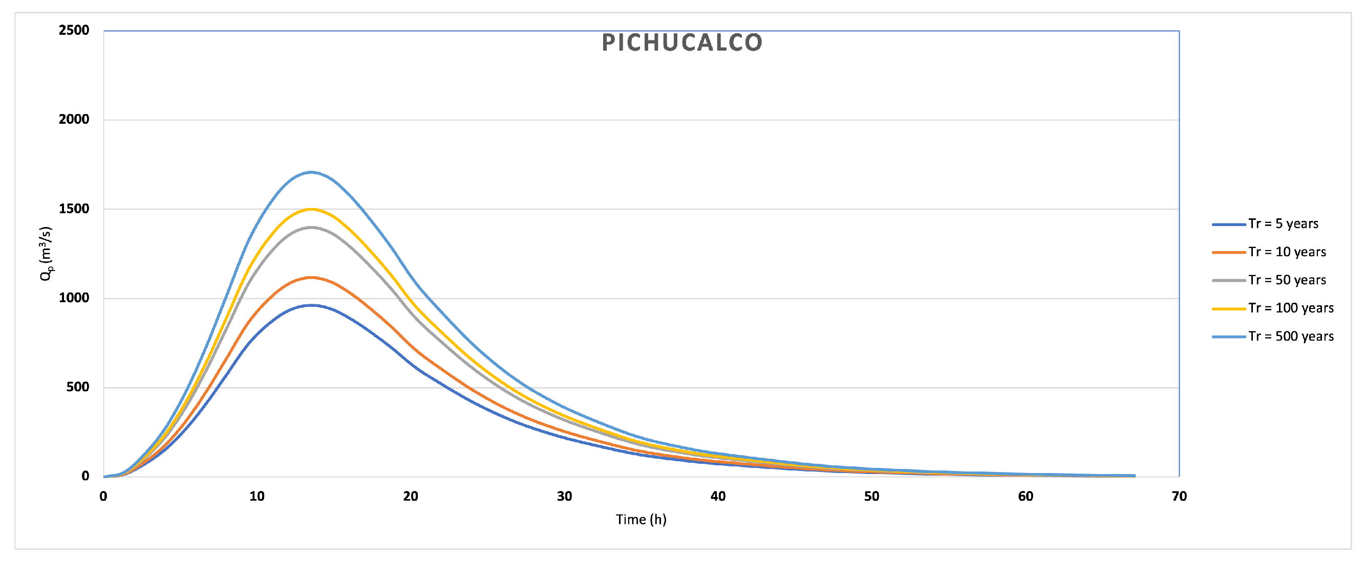
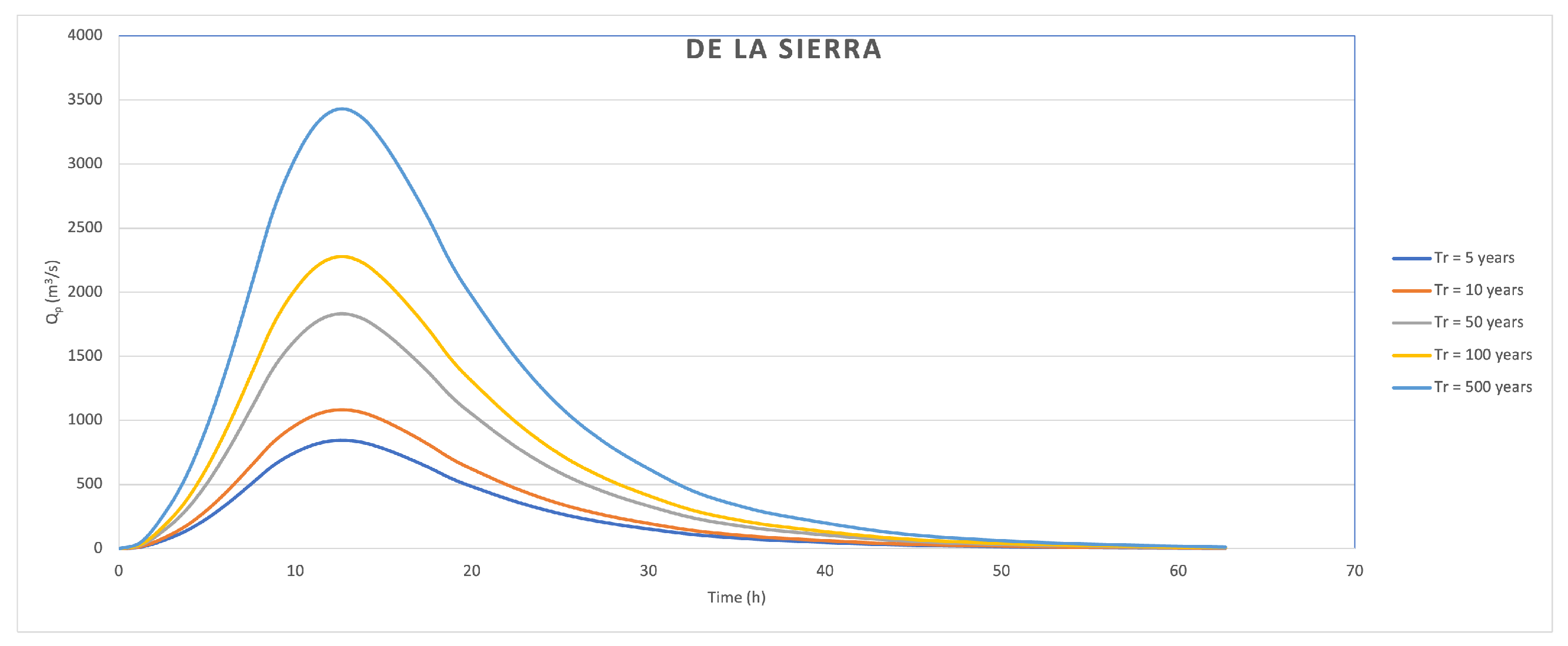
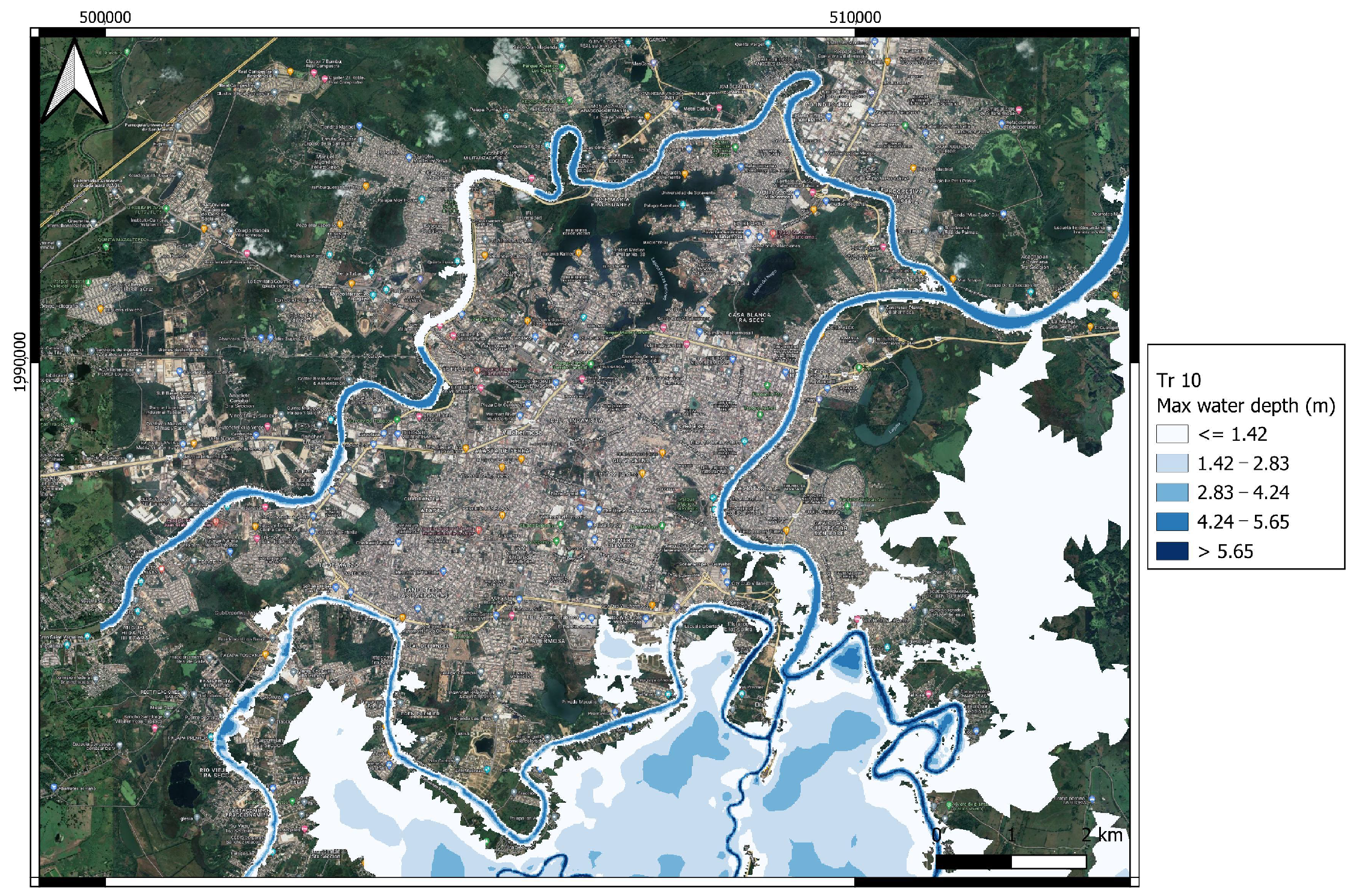
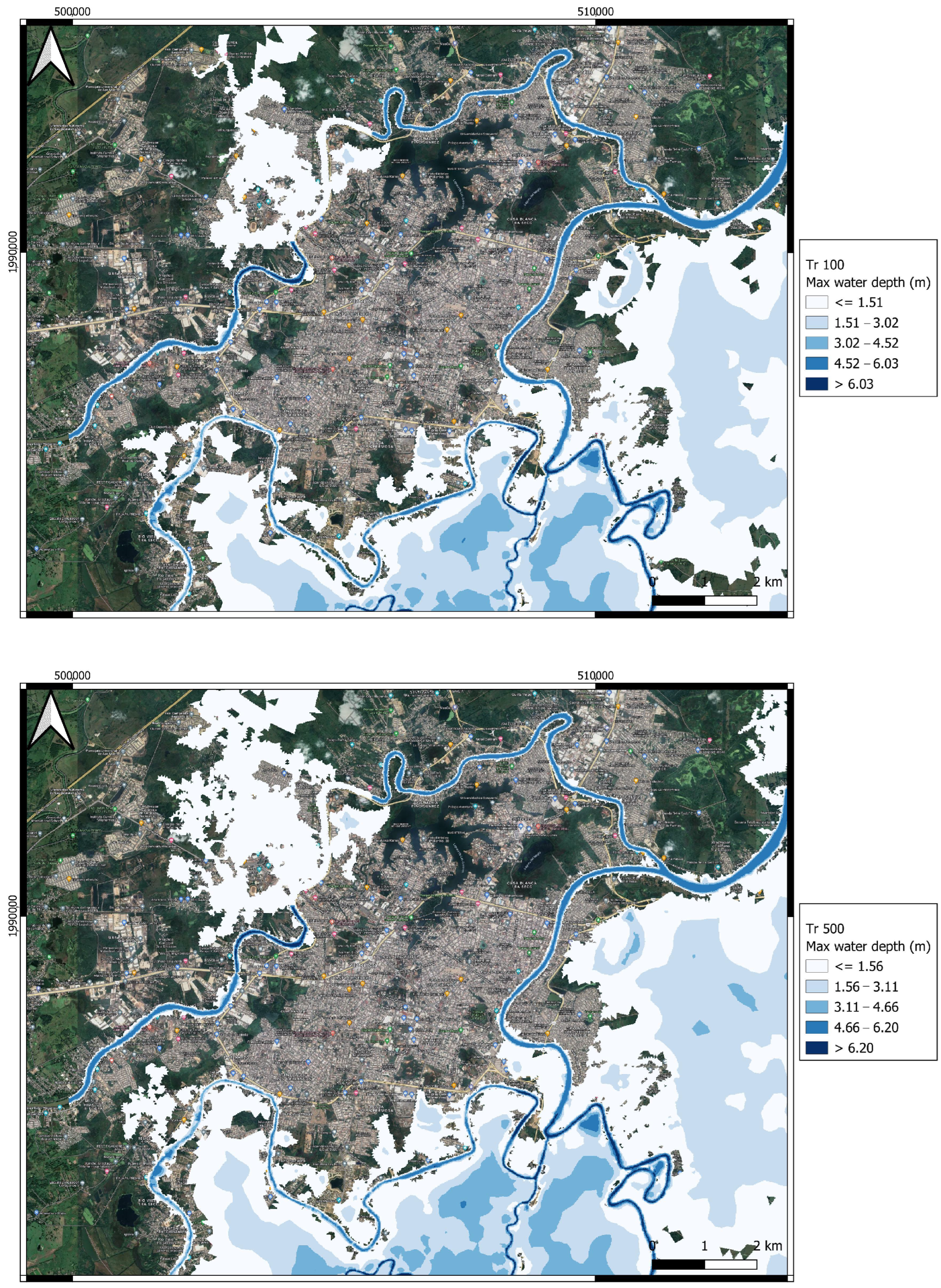
Results of this study show that the portions of Villahermosa most impacted by the effects of floods in terms of economic losses are located in the south near the Grijalva and Viejo Mezcalapa rivers, and in the north those located on the banks of the Carrizal river. For frequent precipitation scenarios (return periods of less than 100 years), these areas are already subject to flooding with water levels exceeding 2 m (Figure 8). These results are validated by local reports which warn the population every year as the rainy season approaches. In fact, the rainy season is almost always accompanied by tropical storms that cause an increase in rainfall intensity every year. For this reason, the Federal Government of the state of Tabasco, together with Civil Protection personnel, meet to define the actions to be taken to help the population in the event of flooding [50], before the rains begin. These meetings are intended to establish the strategies and government actions to face the forecasts provided by the National Water Commission (CONAGUA), regarding the number and category of tropical cyclones that are expected to occur, both in the Pacific and in the Atlantic Oceans. From hydraulic simulations results obtained in this work, it appears that the increase in the return period results in an increase in flood levels that can exceed 4 m (
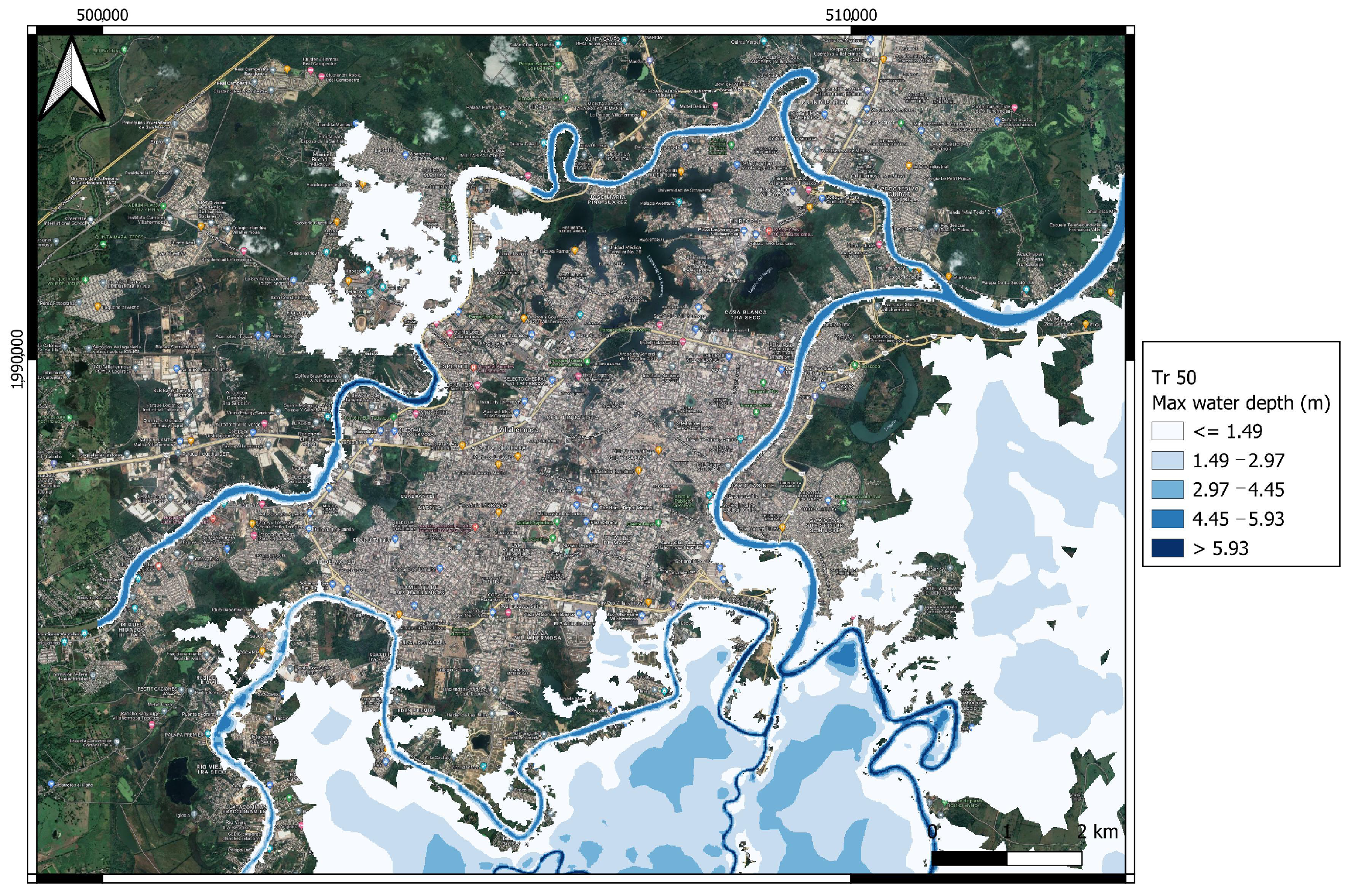
Figure 9). Even these results are plausible if they are associated with the extreme weather phenomena, originating from the combination of storms, cold fronts and cyclones, which in the past caused the disastrous floods whose effects are known.
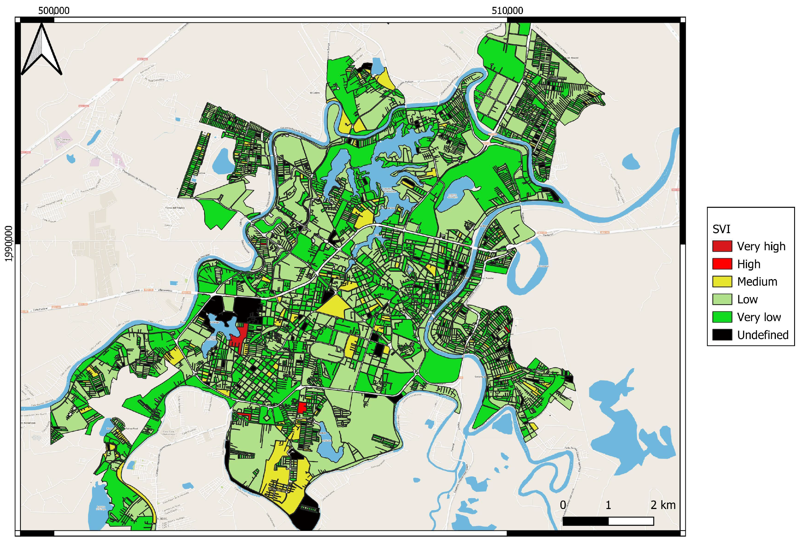
The analysis of the social vulnerability indexes showed that most of the urban districts that conform Villahermosa, have low vulnerability (
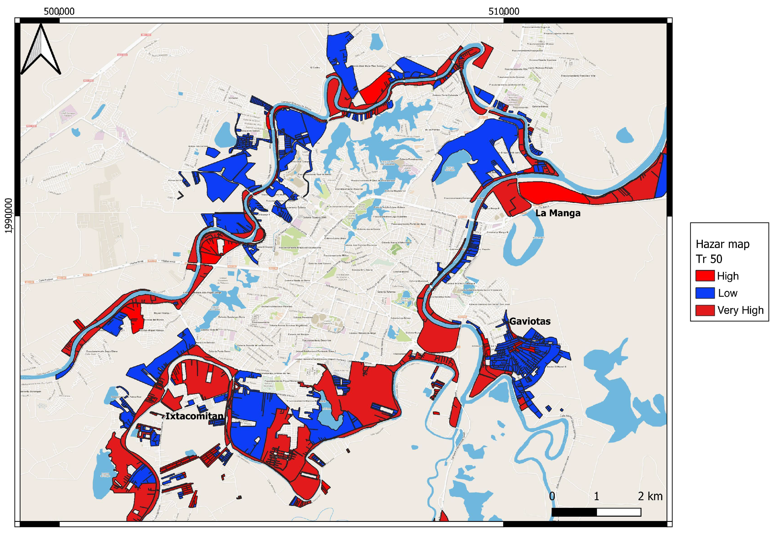
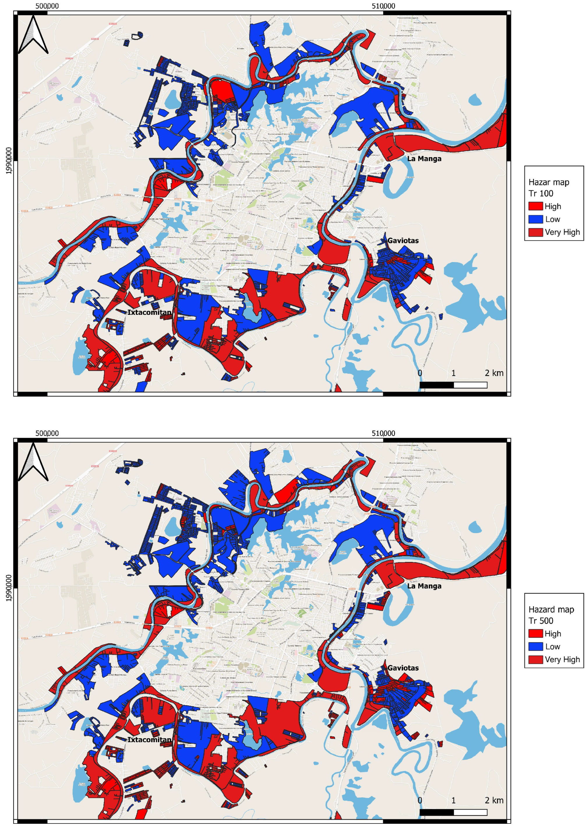
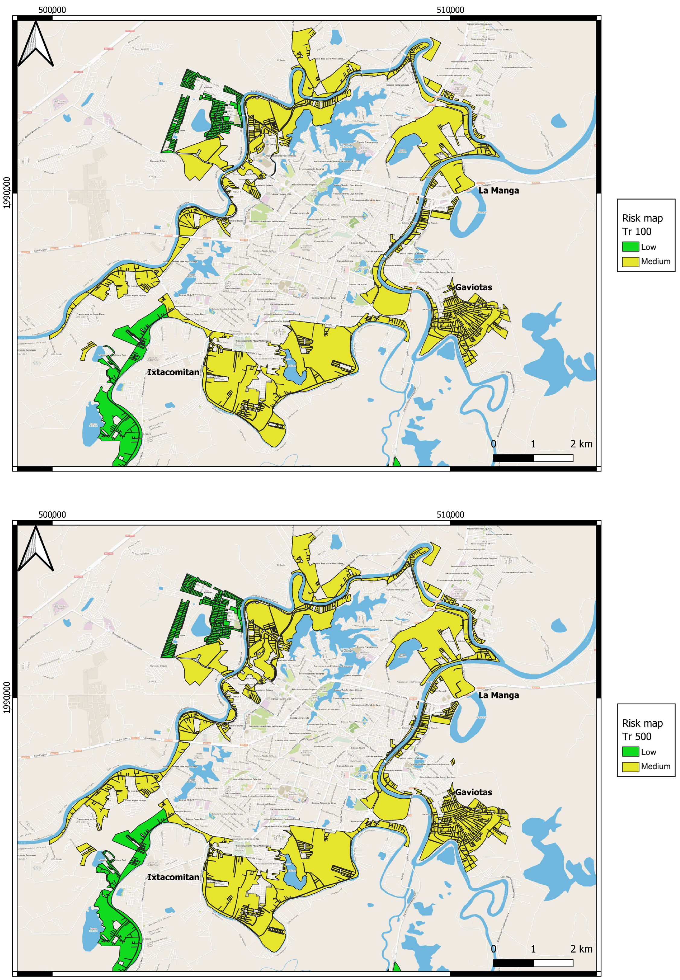
Figure 11). This means that the majority of inhabitants living in Villahermosa have access, at least minimal, to medical services (public and private), education is, at least, at the elementary school level, most of the houses have a water supply, and finally, the majority of people are economically active, i.e., there is little economic dependence. These data come from the analysis of the social vulnerability parameters available in the sources cited in the previous paragraphs. The authors of this work are aware that the database used does not include all the social vulnerabilities that influence the study area, and the available data is not complete. Therefore, we consider that the vulnerability of city’s districts susceptible to flooding may be underestimated. The vulnerability of the areas that periodically remain flooded is most likely higher than that calculated in this work. For this reason, future studies dedicated to more precisely e completely identifying the vulnerability indexes of the area are pivotal. Despite this, results of this study show that areas exposed to flooding show a high hazard based on the damage classification corresponding to the hydraulic thresholds of water velocity and depth given in Table 8. Maps of Figure 12 and Figure 13 show that the districts most likely to suffer flood damage are Ixtacomitán, Gaviotas and La Manga. These are the sections of the city that actually suffer the most from the effects of rains, every year. This is due to their position close to the river branches, but also to an inadequate water drainage system to dispose of excess water. During the 2020 flood, the Mezcalapa river flooded the Ixtacomitan section, leaving it underwater for about two weeks, causing major problems concerning lack of food and the onset of diseases caused by mosquitoes [51]. As a result of the flooding, the Gaviotas section was also underwater for a month. The Gaviotas, located on a southern bank of the Grijalva, has undergone a process of change from a municipal fraction to an urban district in a few years, which has led to the subdivision and sale of lands on the river banks and near water bodies. Furthermore, irregular urban settlements were legally authorized during this urbanization process. While on the one hand, the authorities urged the abandonment of these lands, on the other they offered regularizations, supplies of drinking water and retaining walls for excess water [52]. The same process was undertaken at the La Manga district which, at the hands of the Secretariat of Agrarian Reform in 1982, underwent the expropriation of 33 hectares of municipal land that were subsequently sold at very low cost, thus favoring the settlement of communities in areas at risk of flood.
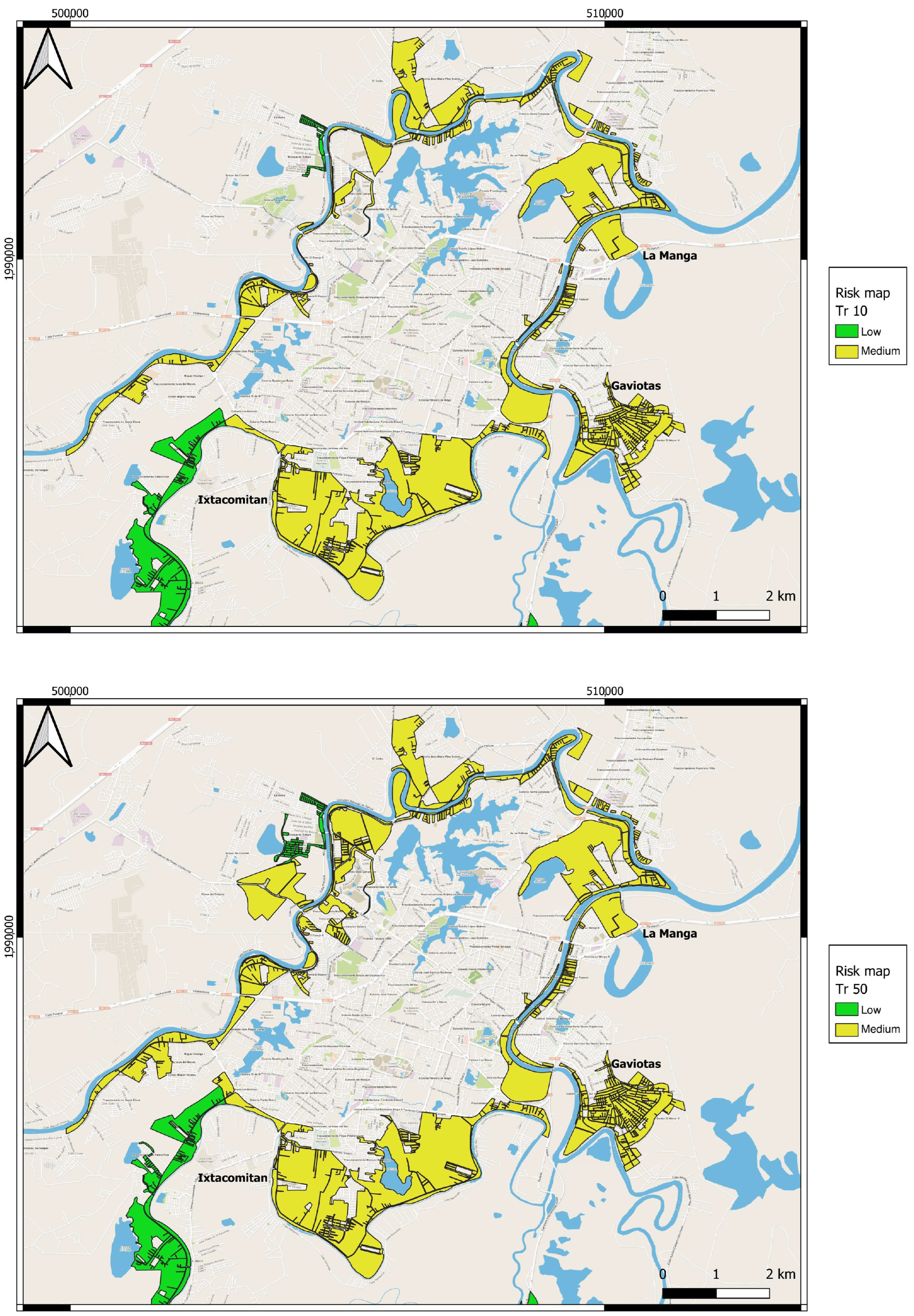
From the risk maps shown in Figure 14 and Figure 15, it appears that the areas most exposed to flooding are affected by a medium risk index, even for simulated scenarios of high return periods. This classification is sensitive to the construction of the vulnerability indexes and to the variables used for this purpose. As previously commented, the construction of the vulnerability map is affected by the limitations imposed by the lack of complete information to define the socio-economic and demographic variables. For many municipal units in the country, there are little or no relevant data in the national statistical censuses. This could be due to a lack of funds to finance this type of research, to the fact that the country is very large, and the investigations are ongoing but do not yet cover the entire territory. However, this circumstance makes it impossible to find fundamental information such as the existence of civil protection institutions on site, perception of risk by the inhabitants, plans and programs to support the population in the event of flooding. Having this information, the vulnerability values calculated for Villahermosa could be higher. In any case, the calculated damage expected annually, show that more than 33,000 people would be affected by floods for an economic damage of more than MXN 250 million, which correspond to more than USD 14 million.

5. Conclusions

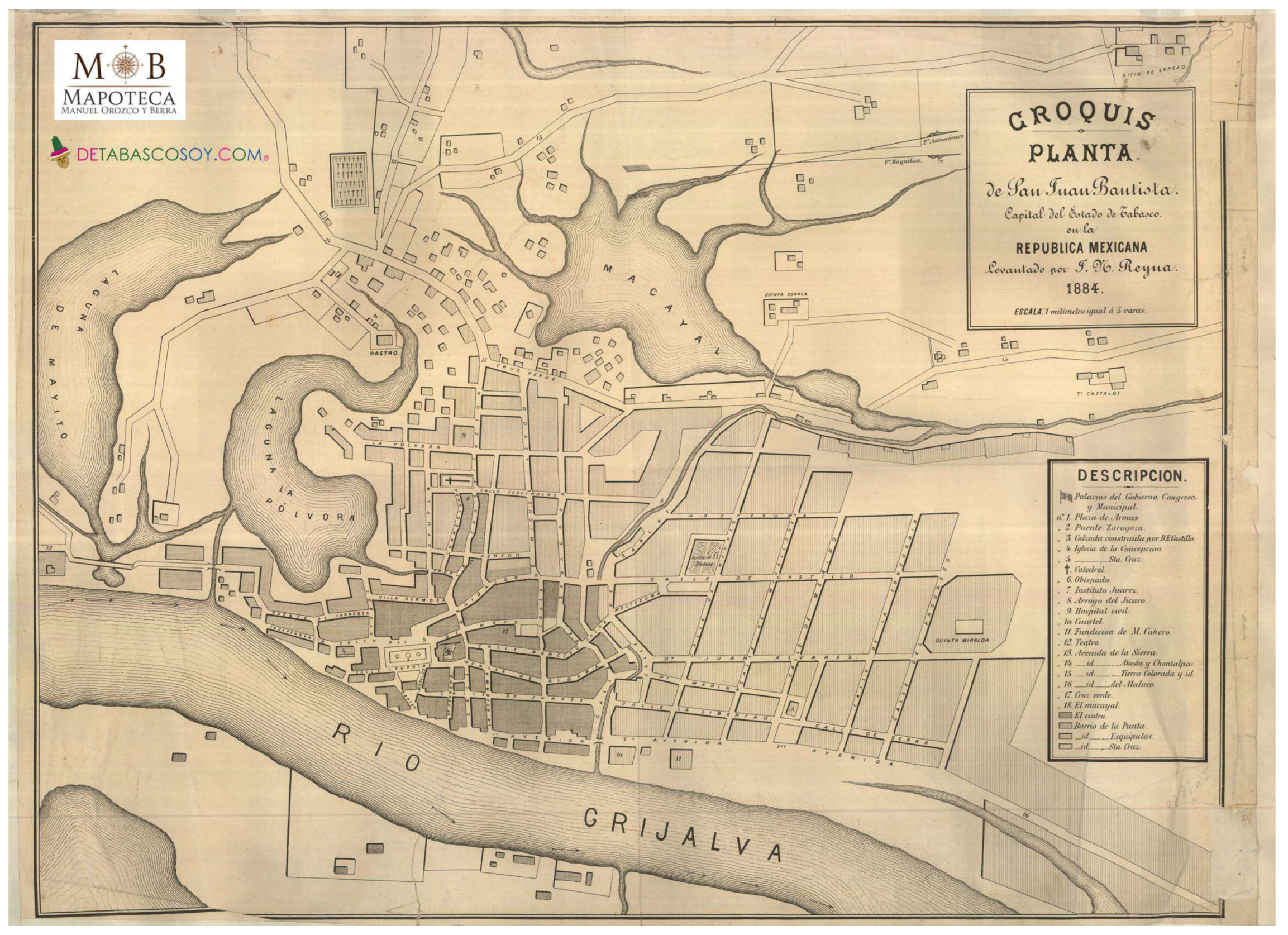
As anticipated and described in the introduction, the Villahermosa problem with respect to flooding has distant roots. Since even before it was constituted into urban districts and before the first dam of the Grijalva Hydroelectric Complex came into operation in 1964, the territory was periodically flooded causing damage to crops and farm houses. The original layout of the city of Villahermosa shows that the Grijalva river was wider than can be seen now (Figure 16).
The dock was located close to the original and main market of the city, and people who wanted to sell and buy their products would arrive via long, shallow boats [53]. Currently, this area is now three-to-four blocks away from the riverbank, however still within the downtown area of the city which encompasses the current dock of the Grijalva, and the area known as the Malecon. The reduction in width of the river that led to the current distance of the market from the river was caused by the draining of the Macayal and the La Polvora lagoons and the land used for construction. In recent years, the impact of floods has increased due to the construction of dams, their malfunctions, and poor urban planning. Hydraulic simulations in this study reveal that the most severely affected areas in the city experience prolonged and deep flooding, and these areas tend to be inhabited by marginalized communities, heightening their vulnerability and risk. Relocating to safer districts is not feasible for these populations without external financial assistance. Moreover, there is uncertainty about the risk perception of residents in these flood-prone zones. Historically, the people of Villahermosa were more aware of the risks and adapted their homes accordingly, but this perception has evolved. Today, various factors, such as cost and trends, lead people to live in flood-prone areas.
Risk maps, like those presented in this study, can certainly act as a tool to educate and create awareness about flooding and its consequences [11]. In Europe, as a result of severe floods that occurred in the 1990s, information systems were developed through the use of risk maps that describe the hazard and impact of floods, fundamental elements for populations at risk to be able to protect themselves and coexist responsibly with the environment [54]. Creating risk maps for Villahermosa, given the current available data, is a challenging undertaking. However, this study serves as an initial step to stimulate further research focused on developing comprehensive databases for constructing precise risk maps in Villahermosa and other flood-prone areas in Mexico. The goal is to lay the groundwork for promoting greater public awareness and informed territorial policies regarding flood risks. In Mexico, there is a lack of a dedicated disaster prevention policy for natural events [22]. This deficiency is possibly due to the National Civil Protection System’s relatively recent establishment following the 1985 earthquake in Mexico City. Moreover, the decision-making process during disasters is decentralized, and local administrations have limited capabilities for hazard assessment and civil protection. To address these issues, the creation and implementation of national-level risk maps are crucial for flood disaster prevention in the country.
The methodology in this study forms a strong foundation for flood risk management, community safety, and sustainable development. It presents a vital tool for the scientific community in addressing hydrological hazards. Moreover, it enables precise identification of flood-prone areas, facilitating flood event prediction and mitigation planning. Additionally, it aids in estimating the financial impact of floods, empowering the scientific community to develop loss-reduction strategies. Furthermore, it supports the evaluation of current public policies and the creation of more effective ones.

Author Contributions

Conceptualization, M.C. and R.B.; methodology, M.C., R.B. and L.C.; software, M.C., R.B. and L.C.; validation, M.C., R.B., L.C. and M.d.l.O.C.-C.; formal analysis, M.C., R.B., L.C. and M.d.l.O.C.-C.; investigation, M.C. and R.B.; resources, M.C. and R.B.; data curation, M.C., R.B. and L.C.; writing—original draft preparation, R.B.; writing—review and editing, M.C., R.B., L.C. and M.d.l.O.C.-C.; visualization, M.C. and R.B.; supervision, R.B.; project administration, R.B. All authors have read and agreed to the published version of the manuscript.

Funding

This research received no external funding.

Institutional Review Board Statement

Not applicable.

Informed Consent Statement

Not applicable.

Data Availability Statement

The data presented in this study are contained within the article.

Conflicts of Interest

The authors declare no conflict of interest.

References

  1. de la Garza, M.; Izquierdo, A.L.; León Cázares, C. Relaciones Histórico-Geográficas de la Alcaldía Mayor de Tabasco: Relación de la Provincia de Tabasco Relación de la Villa de Santa María de la Victoria; Representación del Gobierno del Estado de Tabasco: Tabasco, Mexico, 1988. [Google Scholar]
  2. Aparicio, J.; Martínez-Austria, P.F.; Güitrón, A.; Ramírez, A.I. Floods in Tabasco, Mexico: A diagnosis and proposal for courses of action. J. Flood Risk Manag. 2009, 2, 132–138. [Google Scholar] [CrossRef]
  3. Emanuel, K.A. Downscaling CMIP5 Climate Models Shows Increased Tropical Cyclone Activity over the 21st century. Proc. Natl. Acad. Sci. USA 2013, 110, 12219–12224. [Google Scholar] [CrossRef] [PubMed]
  4. Hoeppe, P. Trends in Weather Related Disasters - Consequences for Insurers and Society. Weather Clim. Extremes 2016, 11, 70–79. [Google Scholar] [CrossRef]
  5. Arreguín-Cortéz, F.I.; Rubio-Gutiérrez, H.; Domínguez-Mora, R.; de Luna-Cruz, F. Análisis de las inundaciones en la planicie tabasqueña en el periodo 1005–2010. Tecnología y Ciencias del Agua 2014, 5, 5–32. [Google Scholar]
  6. PICI. Available online: http://sinat.semarnat.gob.mx/dgiraDocs/documentos/tab/estudios/2003/27TA2003H0004.html (accessed on 27 March 2023).
  7. PHIT. Available online: http://www.conagua.gob.mx/conagua07/contenido/Documentos/LIBROS%20BLANCOS/CONAGUA-01%20Programa%20Integral%20de%20Tabasco%20(PIHT).pdf (accessed on 28 March 2023).
  8. Declaratoria de desastre natural por la ocurrencia de inundaciones pluvial y fluvial del 26 de agosto al 5 de septiembre de 2010, en 12 municipios del Estado de Tabasco. Available online: https://dof.gob.mx/nota_detalle.php?codigo=5159332&fecha=14/09/2010#gsc.tab=0 (accessed on 29 March 2023).
  9. Inundaciones de 2020 en Tabasco. Available online: https://preparecenter.org/wp-content/uploads/2022/08/PERC_Mexico_ESP.pdf (accessed on 29 March 2023).
  10. Kron, W. Keynote lecture: Flood risk = hazard × exposure × vulnerability. In Flood Defense 2002; Wu, B., Wang, Z.-Y., Wang, G., Huang, G.G.H., Fang, H., Huang, J., Eds.; Science Press: New York, NY, USA, 2002. [Google Scholar]
  11. Lundgren, R.E.; McMakin, A.H. Risk Communication. A Handbook for Communicating Environmental, Safety and Health Risks, 4th ed.; Wiley: Hoboken, NJ, USA, 2009. [Google Scholar]
  12. Dransch, D.; Rotzol, H.; Poser, K. The contribution of maps to the challenges of risk communication to the public. Int. J. Dig. Earth 2010, 3, 292–311. [Google Scholar] [CrossRef]
  13. de Moel, H.; van Alphen, J.; Aerts, J.C.J.H. Flood maps in Europe—Methods, availability and use. Nat. Hazards Earth Syst. Sci. 2009, 9, 289–301. [Google Scholar] [CrossRef]
  14. EU Flood Directive, European Commission 2007. Available online: https://environment.ec.europa.eu/topics/water/floods_en (accessed on 7 July 2023).
  15. NFIP (National Flood Insurance Program). Program Description, Federal Emergency Management Agency. 2002. Available online: https://www.fema.gov/pdf/floodplain/nfip_sg_unit_2.pdf (accessed on 7 July 2023).
  16. Jonkman, S.N.; van Gelder, P.H.A.J.M.; Vrijling, J.K. An overview of quantitative risk measures for loss of life and economic damage. J. Hazard Mater. 2003, 99, 1–30. [Google Scholar] [CrossRef]
  17. Burningham, K.; Fielding, J.; Thrush, D. ‘It’ll never happen to me’: Understanding public awareness of local flood risk. Disasters 2008, 32, 216–238. [Google Scholar] [CrossRef]
  18. Sermet, Y.; Demir, I. Virtual and augmented reality applications for environ- mental science education and training. In New Perspectives on Virtual and Augmented Reality: Finding New Ways to Teach in a Transformed Learning Environment; Linda, D., Ed.; Routledge: London, UK, 2020; p. 322. [Google Scholar]
  19. CONAGUA, Lineamientos Para la Elaboración de Mapas de Peligro por Inundación. 2014. Available online: https://www.gob.mx/cms/uploads/attachment/file/469330/Lineamientos__para_la_elaboraci_n_de_mapas_de_peligro_por_inundaci_n.pdf (accessed on 19 May 2023).
  20. Sistema Nacional de Información Sobre Riesgos. Available online: http://atlasnacionalderiesgos.gob.mx/archivo/visor-capas.html (accessed on 7 July 2023).
  21. Evers, M. Participation in Flood Risk Management. An Introduction and Recommendations for Implementation; Centrum för Klimat och Säkerhet, Karlstads Universitet: Karlstad, Sweden, 2012. [Google Scholar]
  22. Bonasia, R.; Lucatello, S. Linking Flood Susceptibility Mapping and Governance in Mexico for Flood Mitigation: A Participatory Approach Model. Atmosphere 2019, 10, 424. [Google Scholar] [CrossRef]
  23. Osti, R.; Tanaka, S.; Tokioka, T. Flood hazard mapping in developing countries: Problems and prospects. Disaster Prev. Manag. 2008, 17, 104–113. [Google Scholar] [CrossRef]
  24. Moser, C.; Satterthwaite, D. Towards Pro-poor Adaptation to Climate Change in the Urban Centres of Low- and Middle- income Countries, Climate Change and Cities Discussion Paper 3. In Human Settlements Discussion Paper Series; Human Settlements Programme International Institute for Environment and Development (IIED): London, UK, 2008; p. 50. [Google Scholar]
  25. Adger, N.W. Social Capital, Collective Action, and Adaptation to Climate Change. Econ. Geogr. 2003, 79, 387–404. [Google Scholar] [CrossRef]
  26. Flanagan, B.E.; Gregory, E.W.; Hallisey, E.J.; Heitgerd, J.L.; Lewis, B. A Social Vulnerability Index for Disaster Management. J. Homel. Secur. Emerg. Manag. 2011, 8, 0000102202154773551792. [Google Scholar] [CrossRef]
  27. Tascón-González, L.; Ferrer-Julià, M.; Ruiz, M.; García-Meléndez, E. Social Vulnerability Assessment for Flood Risk Analysis. Water 2020, 12, 558. [Google Scholar] [CrossRef]
  28. Perevochtchikova, M.; Lezama, J. Causas de un desastre: Inundaciones del 2007 en Tabasco. J. Lat. Am. Geogr. 2010, 2, 73–98. [Google Scholar] [CrossRef]
  29. INEGI: Síntesis de Información Geográfica del Estado de Tabasco. Available online: http://internet.contenidos.inegi.org.mx/contenidos/productos/prod_serv/contenidos/espanol/bvinegi/productos/historicos/2104/702825223939/702825223939_2.pdf (accessed on 10 March 2023).
  30. Areu-Rangel, O.S.; Cea, L.; Bonasia, R.; Espinosa-Echavarria, V.J. Impact of Urban Growth and Changes in Land Use on River Flood Hazard in Villahermosa, Tabasco (Mexico). Water 2019, 11, 304. [Google Scholar] [CrossRef]
  31. Base de datos climatologica nacional (SISTEMA CLICOM). Available online: http://clicom-mex.cicese.mx/ (accessed on 19 April 2023).
  32. Información Estadística Climatológica. Available online: https://smn.conagua.gob.mx/es/climatologia/informacion-climatologica/informacion-estadistica-climatologica (accessed on 19 April 2023).
  33. Anderson, T.W.; Darling, D.A. Asymptotic Theory of Certain “Goodness of Fit” Criteria Based on Stochastic Processes. Ann. Math. Statist. 1952, 23, 193–212. [Google Scholar] [CrossRef]
  34. Laio, A. Cramer–von Mises and Anderson-Darling goodness of fit tests for extreme value distributions with unknown parameters. Surf. Water Clim. 2004, 40, 10. [Google Scholar] [CrossRef]
  35. Ramírez Orozco, A.I.; Aldama Rodríguez, A. Análisis de frecuencias conjunto para la estimación de avenidas de diseño; Asociación Mexicana de Hidráulica, IMTA: Mexico, 2000; p. 174. [Google Scholar]
  36. Del Ángel González, M.; Domínguez Mora, R. Ecuaciones universales ajustadas para el cálculo de lluvias máximas de corta duración. GEOS 2013, 33, 332–349. [Google Scholar]
  37. Bell, F.C. Generalized rainfall duration-frequency relationships. J. Hydraul. Div. 1969, 95, 311–327. [Google Scholar] [CrossRef]
  38. Soulis, K.X. Soil Conservation Service Curve Number (SCS-CN) Method: Current Applications, Remaining Challenges, and Future Per-spectives. Water 2021, 13, 192. [Google Scholar] [CrossRef]
  39. Bladé, E.; Cea, L.; Corestein, G.; Escolano, E.; Puertas, J.; Vázquez-Cendón, J.; Dolz, J.; Coll, A. IBER: Herramienta de simulación numérica de flujo en ríos. Rev. Int. Métodos Numer. para Cálc. y Diseño en Ing. 2014, 30, 1–10. [Google Scholar] [CrossRef]
  40. Fraga, I.; Cea, L.; Puertas, J. Effect of rainfall uncertainty on the performance of physically-based rainfall-runoff models. Hydrol. Process. 2018, 33, 160–173. [Google Scholar] [CrossRef]
  41. Cea, L.; Bladé, E. A simple and efficient unstructured finite volume scheme for solving the shallow water equations in overland flow applications. Water Resour. Res. 2015, 51, 5464–5486. [Google Scholar] [CrossRef]
  42. Continuo de Elevaciones Mexicano (CEM). Available online: https://www.inegi.org.mx/app/geo2/elevacionesmex/ (accessed on 25 April 2023).
  43. Arreguín Cortés, F.I.; López Pérez, M.; Rodríguez López, O.; Montero Martínez, M.J. Atlas de Vulnerabilidad híDrica en México Ante el Cambio Climático; Instituto Mexicano de Tecnología del Agua: Jiutepec, Mexico, 2015; p. 148. [Google Scholar]
  44. Censo de Población y Vivienda 2020. Available online: inegi.org.mx/programas/ccpv/2020/ (accessed on 17 May 2023).
  45. Índices de Marginación 2020. Available online: https://www.gob.mx/conapo/documentos/indexes-de-marginacion-2020-284372/ (accessed on 17 May 2023).
  46. Dorrigo Flood Study. Available online: https://flooddata.ses.nsw.gov.au/related-dataset/dorrigo-flood-study-readme (accessed on 19 May 2023).
  47. Guía báSica para la Elaboración de Atlas Estatales y Municipales de Peligros y Riesgos. Available online: http://centro.paot.org.mx/documentos/cenapred/guia/Capitulo_I.pdf (accessed on 29 May 2023).
  48. Baró-Suárez, J.E.; Díaz-Delgado, C.; Calderón-Aragón, G.; Esteller-Alberich, M.V.; Cadena-Vargas, E. Most probable cost of flood damage in residential areas in Mexico. Tecnol. Cienc. Agua 2011, 2, 2007–2422. [Google Scholar]
  49. Salarios Mínimos. 2022. Available online: https://www.gob.mx/cms/uploads/attachment/file/686336/Tabla_de_Salarios_M_nimos_vigentes_a_partir_del_1_de_enero_de_2022.pdf (accessed on 5 July 2023).
  50. Estrategia de Protección Civil de Tabasco, Ejemplo Nacional. Available online: https://tabasco.gob.mx/noticias/estrategia-de-proteccion-civil-de-tabasco-ejemplo-nacional (accessed on 10 July 2023).
  51. Baja el Agua en Ixtacomitán, Pero Urgen al Gobierno por Ayuda. Available online: https://www.elheraldodetabasco.com.mx/local/baja-el-agua-en-ixtacomitan-pero-urgen-al-gobierno-por-ayuda-6021838.html (accessed on 10 July 2023).
  52. Bautista Sosa, G. La Producción Social del Espacio Urbano en la Ciudad de Villahermosa, Tabasco: El Riesgo por Inundación del Actual Distrito X “Las Gaviotas” (1970–2008). Master’s Thesis, Sustainable Water Management University, El Colegio de San Luis, San Luis Potosí, Mexico, 2017. [Google Scholar]
  53. Martínez, A.C. El Grijalva, un río que fluye en la historia. Signos Históricos 2005, 9, 140–161. [Google Scholar]
  54. Welcome to FloodInfo.ie. Available online: https://www.floodinfo.ie/ (accessed on 11 July 2023).
Figure 1. Location map of the Centro municipality where Villahermosa is located.
Water 15 03969 g001
Figure 2. Map of the sub-basins that drain in Villahermosa. The location of the hydrometric and climatological stations, as well as the inlet points of each river used for the hydraulic simulations are shown.
Water 15 03969 g002
Figure 3. Curve number distribution map for the Carrizal and Viejo Mezcalapa sub-basins.
Water 15 03969 g003
Figure 4. Curve number distribution map for the Pichucalco and de la Sierra sub-basins.
Water 15 03969 g004aWater 15 03969 g004b
Figure 5. Design hydrographs of the Carrizal and Viejo Mezcalapa sub-basins, corresponding to different return periods.
Water 15 03969 g005
Figure 6. Design hydrographs of the Pichucalco and de la Sierra sub-basins, corresponding to different return periods.
Water 15 03969 g006aWater 15 03969 g006b
Figure 7. Location map of the study area. The main land uses identified in the area are indicated (urban vegetation and residential land), as well as the inlet and outlet points to define the boundary hydraulic conditions.
Water 15 03969 g007
Figure 8. Maximum water depth values, obtained from hydraulic simulations for the 10- and 50-year return periods.
Water 15 03969 g008aWater 15 03969 g008b
Figure 9. Maximum water depth values, obtained from hydraulic simulations for the 100- and 500-year return periods.
Water 15 03969 g009
Figure 10. Maximum water velocities, obtained from hydraulic simulations for (a) 10-year return period and (b) 500-year return period.
Water 15 03969 g010
Figure 11. Social Vulnerability Index Map for Villahermosa.
Water 15 03969 g011
Figure 12. Hazard Map of Villahermosa for the 10- and 50-year return periods.
Water 15 03969 g012aWater 15 03969 g012b
Figure 13. Hazard Map of Villahermosa for the 100- and 500-year return periods.
Water 15 03969 g013
Figure 14. Risk Map of Villahermosa for the 10- and 50-year return periods.
Water 15 03969 g014
Figure 15. Risk Map of Villahermosa for the 100- and 500-year return periods.
Water 15 03969 g015
Figure 16. Sketch of San Juan Bautista (today Villahermosa) in 1884.
Water 15 03969 g016
Table 1. Morphological and hydrological parameters of the sub-basins.
CarrizalViejo MezcalapaPichucalcode la Sierra
Length of the channel (km)36.3577.34146.37141.60
Average slope of the channel (%)0.020.061.451.67
Basin area (km 2 )99.8470.91266.91003.8
Maximum elevation of the channel (m)176021372373
Average elevation of the channel (m)133510731191
Concentration time t c (h)28.0332.8415.7514.54
Delay time t r (h)16.8219.79.458.72
Peak time t p (h)22.1125.4313.4212.53
Base time t b (h)59.0467.935.8233.47
Table 2. Fit standard errors calculated in the frequency analysis of precipitation data, for the Carrizal river sub-basin.
Distribution FunctionMomentsMaximum Likelihood
Normal11.6411.64
GEV7.64
Gumbel6.355.53
Table 3. Annual maximum precipitations ( h p ), excess precipitations ( P e ) and design flows ( Q d ) for every basin and 12 return periods from T = 2 years to T = 500 years.
Return Period (Years) h p (mm) P e (mm) Q d (mm 3 /s)
T = 254.10320.00118.773
T = 571.36932.96030.937
T = 1082.80142.19939.608
T = 2093.76651.40948.253
T = 50107.95963.71359.801
CarrizalT = 100118.59573.15368.662
T = 200129.19282.70777.629
T = 500143.17395.49489.631
T = 261.20614.87957.302
T = 578.05425.19597.028
T = 1087.93231.896122.833
T = 2096.55238.053146.547
T = 50106.58845.528175.331
MezcalapaT = 100113.35950.730195.365
T = 200119.52755.567213.992
T = 500126.86661.430236.574
T = 283.65034.631680.256
T = 5102.13648.995962.419
T = 10111.80856.8721117.151
T = 20119.79363.5241247.813
T = 50128.77871.1461397.537
PichucalcoT = 100134.76676.2981498.733
T = 200140.24681.0571592.209
T = 500146.88786.8751706.507
T = 281.06632.759545.696
T = 5104.23750.747845.346
T = 10121.44964.9851082.517
T = 20140.80581.6181359.589
T = 50172.741110.0661833.487
de la SierraT = 100201.961136.8522279.684
T = 200233.265166.0942766.799
T = 500275.222205.8983429.851
Table 4. Optimal values of cell size, roughness and simulation times, adopted to simulate flood scenarios.
Land UseRoughnessCell Size (m)
Residential0.850
Urban vegetation0.08200
Water bodies0.02100
River0.03515/25
Total simulation time 259,200 (s)/72 (h)
Time step (s) 2700
Table 5. Indicators selected for the construction of the SVI.
CategoryIndicators
HealthProportion of doctors per 1000 inhabitants
Infant mortality rate
Percentage of population that does not rely on public health services
EducationIlliteracy rate
Average level of education
HousingPercentage of homes without piped water
Percentage of houses without drainage
Housing deficit
Percentage of houses with adobe floors
Employment and incomePercentage of the Economically Active Population (EAP) that receives less than two minimum wages
Dependency ratio (% of dependent population, in relation to the EAP)
PopulationPopulation density (inhabitants per km 2 )
Percentage of indigenous-speaking population
Percentage of population living in towns with fewer than 2500 inhabitants
Table 6. Values of the indicators calculated for the categories Population, Education, Health, Employment, Housing.
DistrictPopulationEducationHealthEmploymentHousing
10.400.300.800.400.40
20.470.300.800.500.33
30.470.300.800.400.33
40.400.400.800.400.30
50.600.300.400.400.33
Table 7. Social vulnerability indexes (SVI) calculated for the five geostatistical districts of Villahermosa.
DistrictAverage of the IndicatorsSVI
10.46Low
20.48Low
30.46Low
40.46Low
50.61Very Low
Table 8. Severity indexes for hazard maps, and corresponding water velocity and depth thresholds.
HazardColorV = Velocity Threshold (m/s)Y = Water Depth Threshold (m)
Very HighRedV > 2Y > 2
HighOrangeV ≤ 21 < Y ≤ 2
MediumYellowV ≤ 20.8 ≤ Y ≤ 1
LowBlueV ≤ 20.3 ≤ Y ≤ 0.8
Very LowGreenV ≤ 2Y ≤ 0.3
Table 9. Risk Index Ranges and Corresponding Risk Levels.
Risk IndexColorRisk Level
0.67 < I R j < 1RedHigh
0.33 < I R j < 0.67YellowMedium
0 < I R j < 0.33GreenLow
Table 10. Potential damage curves equations.
Potential DamageEquation 1
Very high D D H m a x = 247.63 L n ( h ) + 668.44
D D H m i n = 141.36 L n ( h ) + 382.45
D D H m p = 156.92 L n ( h ) + 424.33
High D D H m a x = 289.63 L n ( h ) + 801.56
D D H m i n = 228.58 L n ( h ) + 637.93
D D H m p = 280.51 L n ( h ) + 777.60
Medium—one-story house D D H m a x = 709.63 L n ( h ) + 1976.04
D D H m i n = 544.93 L n ( h ) + 1546.60
D D H m p = 685.51 L n ( h ) + 1913.15
Medium—two-story house D D H m a x = 549.55 L n ( h ) + 1345.57
D D H m i n = 405.03 L n ( h ) + 965.27
D D H m p = 528.39 L n ( h ) + 1289.88
Low—one-story house D D H m a x = 877.28 L n ( h ) + 2479.23
D D H m i n = 797.24 L n ( h ) + 2233.19
D D H m p = 865.56 L n ( h ) + 2443.20
Low—two-story house D D H m a x = 666.15 L n ( h ) + 1632.94
D D H m i n = 595.33 L n ( h ) + 1409.03
D D H m p = 605.70 L n ( h ) + 1441.82
Very low—one-story house D D H m a x = 1521.80 L n ( h ) + 4051.63
D D H m i n = 1210.14 L n ( h ) + 3321.20
D D H m p = 1255.78 L n ( h ) + 3428.17
Very low—two-story house D D H m a x = 1230.35 L n ( h ) + 2850.34
D D H m i n = 939.78 L n ( h ) + 2221.33
D D H m p = 1187.79 L n ( h ) + 2758.22
Notes: 1  D D H m a x : Maximum damage cost in urban area; D D H m i n : Minimum damage cost in urban area; D D H m p : Probable cost in urban area; h: Depth of water flow on the surface. The economic damage is estimated in minimum wage units.
Table 11. Characteristics of the Villahermosa flood-affected area relative to a 10-year return period and expected annual potential damage.
InhabitantsHousing UnitsFloodable Area (km 2 )People with Minimum WagesEconomic Value of Exposed Assets (MXN)Risk IndexRisk
Classification
Villahermosa33,819971713.861,239,027257,023,6990.632Medium
Disclaimer/Publisher’s Note: The statements, opinions and data contained in all publications are solely those of the individual author(s) and contributor(s) and not of MDPI and/or the editor(s). MDPI and/or the editor(s) disclaim responsibility for any injury to people or property resulting from any ideas, methods, instructions or products referred to in the content.

