Article

Impact Evaluation Using Nonstationary Parameters for Historical and Projected Extreme Precipitation

by
Muhammad Usman Khan
1,
Muhammad Wajid Ijaz
2,
Mudassar Iqbal
1,*,
Rizwan Aziz
3,
Muhammad Masood
1 and
Muhammad Atiq Ur Rehman Tariq
1,4,*
1
Centre of Excellence in Water Resources Engineering, University of Engineering and Technology, Lahore 54890, Punjab, Pakistan
2
Environment Protection Department, Government of the Punjab, Lahore 54000, Punjab, Pakistan
3
College of Earth and Environmental Sciences, University of the Punjab, Lahore 54590, Punjab, Pakistan
4
College of Engineering, IT & Environment, Charles Darwin University, Darwin, NT 0810, Australia
*
Authors to whom correspondence should be addressed.
Water 2023, 15(22), 3958; https://doi.org/10.3390/w15223958
Submission received: 27 June 2023 / Revised: 23 July 2023 / Accepted: 27 July 2023 / Published: 14 November 2023
(This article belongs to the Topic Hydrology and Water Resources Management)

Abstract

:
Recent improvements in time series studies of hydro-climatological variables have led to the belief that the effects of nonstationarity are substantial enough to call the idea of traditional stationary approaches into doubt. The mean and variability of annual and seasonal rainfall in Pakistan are changing due to anthropogenic climate change. With the use of stationary and nonstationary frequency analysis techniques, this study set out to assess the impacts of nonstationarity in Southern Punjab, Pakistan, over the historical period of 1970–2015 and the future periods of 2020–2060 and 2060–2100. Four frequency distributions, namely Generalized Extreme Value (GEV), Gumbel, normal, and lognormal, were used. The findings of the nonstationarity impact across Southern Punjab showed different kinds of impacts, such as an increase or reduction in the return level of extreme precipitation. In comparison to other distributions, GEV provided the finest fit. In Bahawalnagar, Bahawalpur, Multan, Rahim Yar Khan and DG. Khan, the annual nonstationarity impacts for the 100-year return level were increased up to 15.2%, 8.7%, 58.3%, 18.7%, and 20%, respectively. Moreover, extreme precipitation was found to be increasing during the historical and projected periods, which may increase floods, while less water availability appeared at a seasonal scale (summer) during 2061–2100. The increased nonstationarity effects emphasized adapting these nonstationarities induced by climate change into the design of water resource structures.

1. Introduction

A comprehensive understanding of extreme precipitation is an important challenge in hydrology. Probability distributions for frequency analysis (FA) are a common technique used by engineers and hydrologists to understand extreme precipitation regimes throughout the world. In accordance with the IPCC’s Sixth Assessment Report, anthropogenic activities have been altering the climate with increasing intensity, resulting in major changes in regional climate and increasingly frequent extreme weather events [1]. The design of major infrastructures, such as urban and highway drainage, flood barriers, hydraulic structures, sewerage systems, and dam spillways, relies on the magnitude and frequency of heavy precipitation events [2]. As a consequence, it is important to understand the annual and seasonal distribution of extreme precipitation events. Frequency analysis calculates the extreme precipitation for a specific return period; however, the methods now in use presuppose that the peak time series are uniformly distributed and independent [3,4], or in other words, without trends and unexpected deviations [5]. In fact, the idea of stationarity has been and continues to be used to build water-related development and flood prevention projects all over the world. The climate system has been stressed in recent decades owing to natural changes in global temperature, and human activity has a potential impact on regional climate, which is eventually deteriorating the natural cycle of water [6]. The hypothesis of stationarity has become widely questionable in the context of regional and global change. However, many studies suggested an increase in the nonstationary nature of climate patterns. Keeping this in mind, various studies have attempted to investigate the validity of this concept in flood regimes in many different parts of the world, taking into account the influence of natural climatic variability [7,8,9,10,11,12,13] or land use changes [14,15,16]. Therefore, there is convincing evidence that the stationarity assumptions must be revised under the changing climate [17], and the development and planning of water resources and the design of hydraulic structures need to be evaluated by considering the nonstationarity approach.
The regional variance in precipitation is intimately related to reliable and precise estimations of global climate trends [18]. Changes in precipitation volume and pattern might have a direct impact on the water resources and agriculture of the affected regions [19]. As a result, knowing the spatiotemporal variance in precipitation at the regional scale is critical in climate monitoring and hydro-climate studies [20]. The spatiotemporal variations of precipitation for various parts of the world have been recorded by several studies [21,22,23,24]. There is increasing consensus that long-term variations in precipitation may affect agricultural and hydrological systems [25], which provide the basis of our understanding of both global and local climate change [26]. These precise and trustworthy precipitation data serve as the foundation for our understanding of regional and global climate change as well as any potential effects on water supplies [27,28]. Warmer temperatures lead to greater water vapor content, resulting in more severe precipitation in seasons, although annual precipitation is modestly reduced [29]. Extreme precipitation events can cause severe flooding, property damage, and potential loss of life, especially in urban areas with high population density [2]. Unfortunately, a lot of recorded data indicates that occurrences of severe precipitation are becoming increasingly common in many parts of the world. For instance, Donat et al. [30], analyzed the data from over 11,000 worldwide weather stations between the years 1951 and 2010, and it is concluded that severe precipitation occurrences increased in both the dry and wet parts of the world. Hence, there is substantial evidence of severe precipitation variations.
Economic losses from weather- and climate-related disasters have increased with large spatial and inter-annual variability. There is a lack of data at the local level on disasters and disaster risk reduction, which can constrain improvements in local vulnerability reduction [31]. Pakistan is listed among the top vulnerable countries to climate change, which is experiencing catastrophic climate extreme events, and these extreme events are predicted to increase in frequency, intensity, and duration. The climate change scenario is alarming because of the existence of climate-change-related risks in Pakistan, including sea level increase, glacial depletion, high average temperatures, floods, and high-frequency droughts, and half of the country’s population is at risk [32]. Moreover, Pakistan has been listed as the eighth most impacted country in the world by extreme occurrences, according to the Global Climate Risk Index (CRI) [33]. In Pakistan, extreme weather events, including heatwaves, intense rainfall, floods, and droughts, have become more frequent and violent during the past few decades [34]. Numerous studies that compared precipitation statistics for various time periods and examined precipitation extremes and mean changes typically used trend analysis (e.g., the Mann–Kendall test and Sen’s slope estimate) [35]. Hence, it is evident that most of the studies remained silent, considering nonstationary approaches in evaluating return levels of extreme precipitation. The Punjab province of Pakistan produces the majority of the nation’s agricultural commodities and is extremely vulnerable to changes in most meteorological parameters due to extreme events [36]. Furthermore, to address the gaps in earlier research, local-scale studies evaluating changes in intense precipitation are necessary. Many investigations have been undertaken over the years to demonstrate how the concept of stationarity (for example, the notion of regular return intervals) may be adversely affected as a result of environmental change [37,38]. For instance, Aziz et al. [39] focuses on the transient inconsistency in yearly as well as seasonal extreme rainfall in Turkey, which was investigated by using stationary and nonstationary frequency approaches. Sertac et al. [40] studied the nonstationary investigation of extreme rainfall and observed that nonstationary (NST) models outperformed the stationary model at the 17 stations. Nashwan et al. [41] investigated how a change in the environment (nonstationarity) affects the average and intensity of annual and seasonal rainfall in Malaysia and the magnitude of maximum rainfall at 2-, 10-, 25-, 50-, and 100-year return periods has increased at most of the stations. In terms of environmental change, the assessment of the recurrence time of exceptional precipitation occurrences according to static assumptions may thus be insignificant. The frequency of extreme temperatures, droughts, floods, and rainfall has risen during the last century [42,43]. However, most studies only used historical and CMIP5 GCMs to assess different aspects of the hydrological cycle, such as atmospheric precipitation [44,45,46,47,48] and surface hydrological processes [49,50]. Therefore, these studies are evident in the validity of historical and future precipitation scenarios and should also be updated with SSP2 and SSP5 scenarios.
Changing climate and land utilization circumstances may modify the probability of hydrodynamically significant occurrences, implying that the characteristics (of location, shape, and scale) of fundamental distributions may vary over time, rendering the view of stationarity unsustainable [39]. The return levels of extreme precipitation can be more accurately predicted for any particular return period from a nonstationary perspective. On the other hand, the predicted return levels are vulnerable to oversights like overestimation or underestimation when nonstationarity is not taken into consideration. This study examines the evaluation of nonstationary impacts for the return levels of extreme precipitation at the local scale.
In this work, we provide an update on nonstationary impacts in return levels of extreme precipitation at the Southern Punjab. Specifically, the aim of this study was (a) to determine the best distribution function under stationary and nonstationary assumptions, and (b) to quantify the nonstationary impacts at historical and projected extreme precipitation. Overall, study findings will aid in predicting the changes in historical and projected extreme precipitation by considering nonstationary parameters in terms of a changing climate.

2. Study Area and Datasets
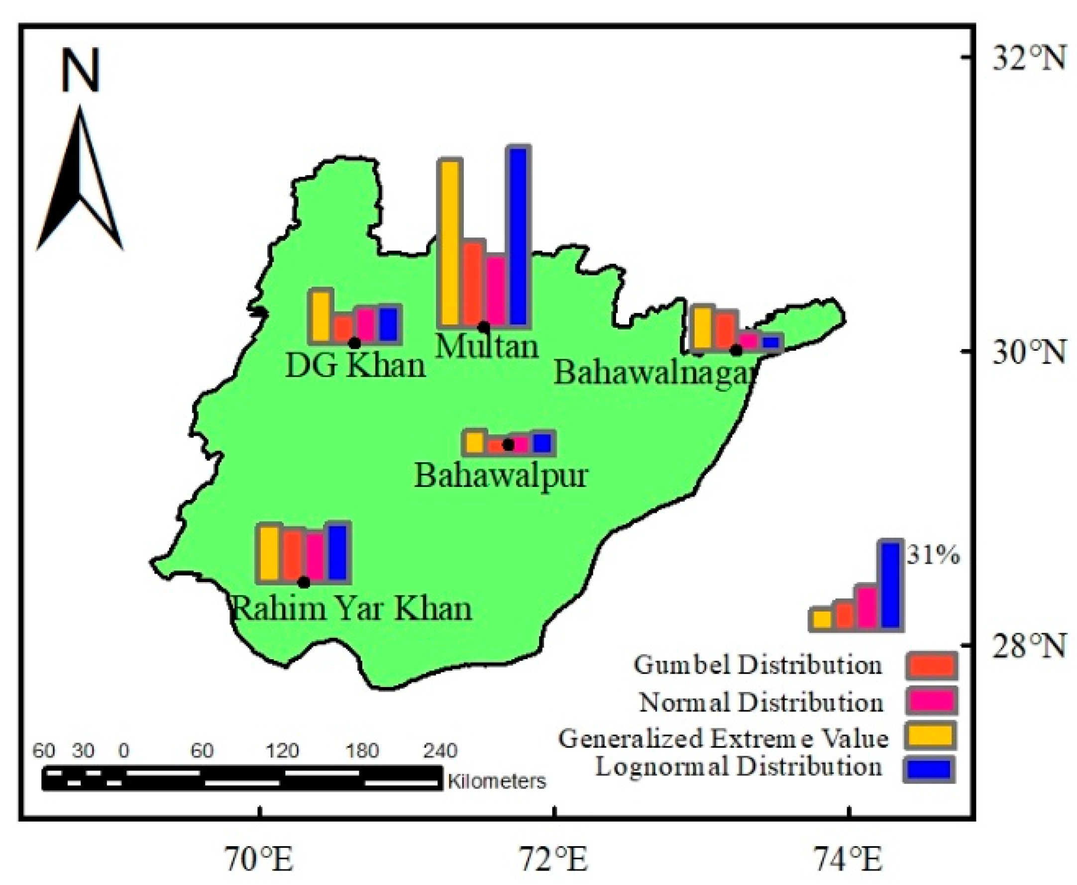
2.1. Study Area

Pakistan geographically lies between 24°–37° N and 60°–75° E in southwest Asia. The country has an area of 8 × 10⁶ km2. The country has a diverse landscape ranging from the Karakoram and Himalayan mountains in the north and northwest, with the agricultural plains of the Indus River basin in the center and the Arabian Sea along the southern coast [51]. The province of Punjab, Pakistan, is the second largest province, and its districts are distributed in the southern, northern, and central parts. This study was carried out in South Punjab, Pakistan and lies between 28.0° to 30.5° North latitude and 69.0° to 73.0° East longitude (Figure 1). The total area of the study region is 205,345 square kilometers. Despite the fact that the region is primarily flat, the southwest includes a few hilly areas. In addition to Cholistan, a desert region of the country, there is a part of the Koh-e-Suleman mountain range that exists towards the west of the study region.
South Punjab experiences a subtropical climate characterized by hot summers and mild winters. The region has two distinct seasons: a hot and dry season from April to June and a monsoon season from July to September. The average maximum and minimum temperature ranges from 38 °C to 45 °C and 25 °C to 30 °C, respectively during the summer period. In the winter, the average maximum and minimum temperatures drop down ranges from 20 °C to 25 °C and 7 °C to 12 °C, respectively. The average annual precipitation varies across different locations within the region. The average annual precipitation in the region ranges between 100 and 400 mm. The majority of rainfall occurs during the monsoon seasons from July to September. During this period, the region receives a significant portion of its annual precipitation. The rest of the year tends to be relatively dry, with sporadic and limited rainfall.

2.2. Datasets

In South Punjab, the impacts of nonstationarities on annual and seasonal min-max precipitation were investigated for the actual period (1970–2015) and for the chosen high-resolution model for the prediction period (2020–2100). Five meteorological stations from the Pakistan Metrological Department (PMD) and five GCM models were used for the analyses that took place in the South Punjab region.
Daily rainfall measurements (1971–2015) were taken from the Pakistan Met Department, and future projections (2020–2100) were taken from the GCM models, which are in phase 6 (CMIP6). (https://esgfnode.llnl.gov/projects/cmip6/ (accessed on 15 January 2023). Numerous researchers analyzed precipitation and maximum and minimum temperature variables using multiple GCM (more than one) because of computational limitations, resolution of data, availability of data against selected emission scenarios, and to compare different models’ performance [52,53,54,55]. For instance, the AWI-CM-1-1-MR model provides both maximum and minimum temperature data at a 100 km resolution, while CESM2, CESM-WACCM, CESM-WACCM-FV2, and CMCC-CM2-SR5 only provide precipitation data at the same resolution. EC-Earth3-AerChem includes all the necessary input variables for only one SSP scenario, and EC-Earth3-CC, HadGEM-GC31-MH, and GFDL-CM4 provide data for two SSP scenarios on a daily basis at a 100 km resolution. Additionally, some of the GCMs, such as FGOALS-3-H, GFDL-C4C192, and SAMO-UNION, do not provide future projections of numerous meteorological inputs. Based on the data required for further hydrological application, we chose the models listed in Table 1.
The climate projections of the five selected models were downloaded under shared socioeconomic pathways (SSP) scenarios 2 and 5. In the current era of industrialization, an immediate drastic decrease in the emission of greenhouse gases is difficult, and it is unlikely to meet this scenario [56]. The scenario SSP2 with medium stabilization forcing scenario and the scenario SSP5 with very high radiative forcing scenario are considered in this study.

3. Methodology

Both stationary and nonstationary probability distributions are applied to estimate the effects of nonstationarities. Precipitation analyses incorporate the GEV, Gumbel, normal, and lognormal distributions. Global Circulation Models (GCMs) have been utilized for future forecast periods, while historical analysis has been performed using observed data. Figure 2 provides an explanatory flowchart for the approach used in this study.

3.1. Statistical Analysis

The initial analysis of studied meteorological stations was calculated, including mean, standard deviation (STD), coefficient of variance (Cv), coefficient of skewness (Cs), and coefficient of kurtosis (Ck) for annual precipitation data. The summary of these statistics is given in Table 2.
The maximum annual mean value of precipitation was found 254 mm at Bahawalnagar in the northeast of the study area. The values of the coefficient of kurtosis and coefficient of skewness varied between −0.59 to 4.08 and 0.42 to 1.67, respectively, of annual precipitation. The values of the coefficient of skewness and kurtosis should be in the range of 0 and 3 for normal distribution. Cs indicated that data on precipitation are positively distributed but with comparable differences among stations. The coefficient of variance was calculated to find out the spatial variability of precipitation at each station. The values of the annual precipitation coefficient of variances varied between 50% and 70%.

3.2. Stationarity in Data Series

The Mann–Whitney U (MWU) test is a non-parametric test developed by Mann and Whitney and is commonly used in frequency analysis of extreme events for the stationarity assumption [57]. Mann–Whitney U Test was performed for the annual and seasonal maximum extreme precipitation. The results stated that data exhibited stationary as significance level alpha = 5% is lesser than the estimated p value as shown in Table 3. Furthermore, the details about the Mann–Whitney U Test can be searched out in the studies of [58,59].

3.3. Stationary and Nonstationary Frequency Analysis

The effects of nonstationarities are computed using both stationary and nonstationary probability distributions. Extreme value distributions are used in hydrology and water resources to examine the probability behavior of severe occurrences like droughts and flooding. The four distributions of generalized extreme value, Gumbel, normal, and lognormal, have been used in this study to carry out the return level for a specific return period. Numerous researchers used these probability distributions for the analysis of return levels of hydro-meteorological variables [39,40,41,60,61,62,63,64]. The analysis of precipitation was carried out for the historical and projected period. The parameters of the distributions are rendered time-dependent by including time as a covariate, allowing for their application in nonstationarity settings [39,65,66]. Coles et al. [67], expressed (the return level is defined as a value that is anticipated to equal or be exceeded with a probability of 1/T once per unit of time (T)) of how return level and return period might alter in nonstationary climate circumstances. Therefore, both stationary and nonstationary GEV, Gumbel, normal, and lognormal probability distributions are applied. The GEV probability distribution function of the nonstationarity form is presented in Equation (1) [65,66].
F   z ,   θ t = e x p     1 + ε   z μ t   σ t 1 ε  
where θ t is a time-dependent set of GEV parameters, which comprises a constant shape parameter ( ε ) and a time-dependent location ( μ t ) and scale ( σ t ) parameters. The shape parameter ( ε ) is typically not modeled as a time-variant parameter since it is more challenging to predict properly [66,67]. Therefore, the location parameter turns µt = µ1+ µ2t, and the scale parameter turns σt = σ1+ σ2t in the case of nonstationary distributions. Moreover, the location and scale parameters under nonstationary conditions are represented by intercept (slope), respectively. Additionally, “t” is the temporal explanatory covariate that causes (µt) and (σt) to be nonstationary for a studied period ranges from one to the entire number of data periods.
The GEV distribution transforms itself into the Gumbel distribution after the shape parameter gets closer to zero. Furthermore, the other two parameter distributions, normal and lognormal, were also applied under both stationary and nonstationary conditions. By reducing the negative log-likelihood function, distributional parameters were evaluated using the maximum likelihood estimation method. The log-likelihood functions for a stationary and nonstationary variant of the GEV distribution are presented in Equations (2) and (3), respectively.
l   ( μ ,   σ ,   ε ,   x )   = n   l o g   σ 1 ε + 1   i = 1 n l o g   1 + ε   x i μ σ i = 1 n l o g   1 + ε   x i μ σ   1 ε  
l   ( μ t ,   σ t ,   ε )   = n   l o g   σ 1 ε + 1   i = 1 n l o g   1 + ε   x i μ t σ t   i = 1 n l o g 1 + ε   x i μ t σ t   1 ε  
where i represents the total number of years from 1 to n and sigma ( σ ) represents the scale parameter of the probability distribution. Equations (4) and (5) can be used to represent the log-likelihood functions for stationary and nonstationary normal distributions, respectively. For both stationary and nonstationary lognormal distributions, the log-likelihood function may be expressed as Equations (6) and (7).
l   ( μ ,   σ ,     x )   = n 2   l n   ( 2   π ) n 2   l n   ( 2   π   σ 2 ) 1 2   σ 2   i = 1 m ( x j μ ) 2
l   ( μ t ,   σ t ,     x )   = n 2   l n   ( 2   π ) n 2   l n   ( 2   π   σ t 2 ) 1 2   σ t 2   i = 1 n ( x j μ t ) ` 2
l   ( μ ,   σ ,     x )   =     n 2   l n   ( 2   π   σ 2 ) i = 1 m l n   ( x i ) i 1 m l n l n     ( x i ) 2   2 σ 2 +   i 1 m l n l n     x i   μ   σ 2 n μ 2 2   σ 2
l   ( μ t ,   σ t ,     x )   =     n 2   l n   ( 2   π   σ t 2 ) i = 1 m l n   ( x i ) i 1 m l n l n     ( x i ) 2   2 σ t 2 +   i 1 m l n l n     x i   μ t   2 σ t 2 n μ t 2 2   σ t 2
Parameter estimation of these distribution functions (with and without the nonstationarity assumption) can be performed using different packages available in the R-Programming. To name a few, these packages include ‘GEVcdn’ by [68], “ismev” by [69], “extremes” such as [70,71]. We opted for “ismev” package, which enables the estimation of distribution parameters using the “Nelder–Mead” algorithm for optimization under stationarity and nonstationarity assumptions. The temporal evolution of parameters is performed by using a time vector as a covariate. Hence, in the case of nonstationary GEV, the estimated location parameter (μt = μ0 + μ1 *t) has two components. The μ0 (first component) is constant (which is analogous to intercept), and μ1 (second component) is time-multiple (analogous to the slope of the time-variant parameter). This makes the whole parameter μt time-variant or nonstationary. Furthermore, the details about the distribution fitting with and without nonstationarity assumptions can be found in [69]. A similar procedure was followed for normal and lognormal distribution fitting under the nonstationarity assumption.
The probability distribution with the lowest negative log-likelihood (NLLH) is projected to offer greater compatibility since the parameters of probability distributions were assessed by minimizing the (NLLH) functions. The return levels for the 100-year return period were evaluated after finalizing the parameters of the distributions for stationary and nonstationary assumptions. The equation used to explain the effects of nonstationarities is expressed as percentage changes between 100-year stationary and nonstationary return values.
Non - stationarity   impacts =   [ n o n   s t a t i o n a r y   r e t u r n   v a l u e s t a t i o n a r y   r e t u r n   v a l u e ] s t a t i o n a r y   r e t u r n   l e v e l × 100
Nonstationarity has an increasing (or decreasing) influence, which means that greater (or lower) return levels develop when nonstationarity were taken under consideration. Greater (or lower) return levels show that nonstationarity has increased or decreased the likelihood of an extreme event recurring within a certain return period.

4. Results

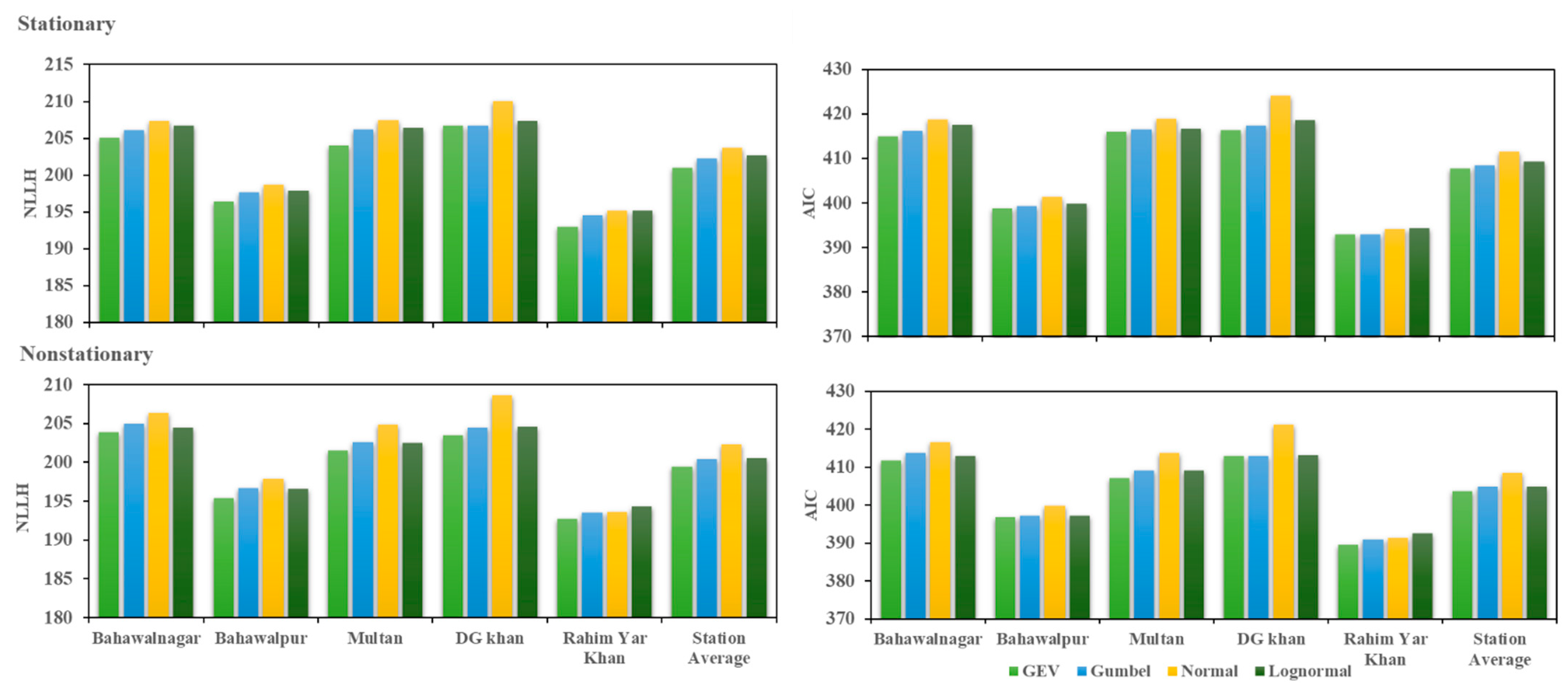
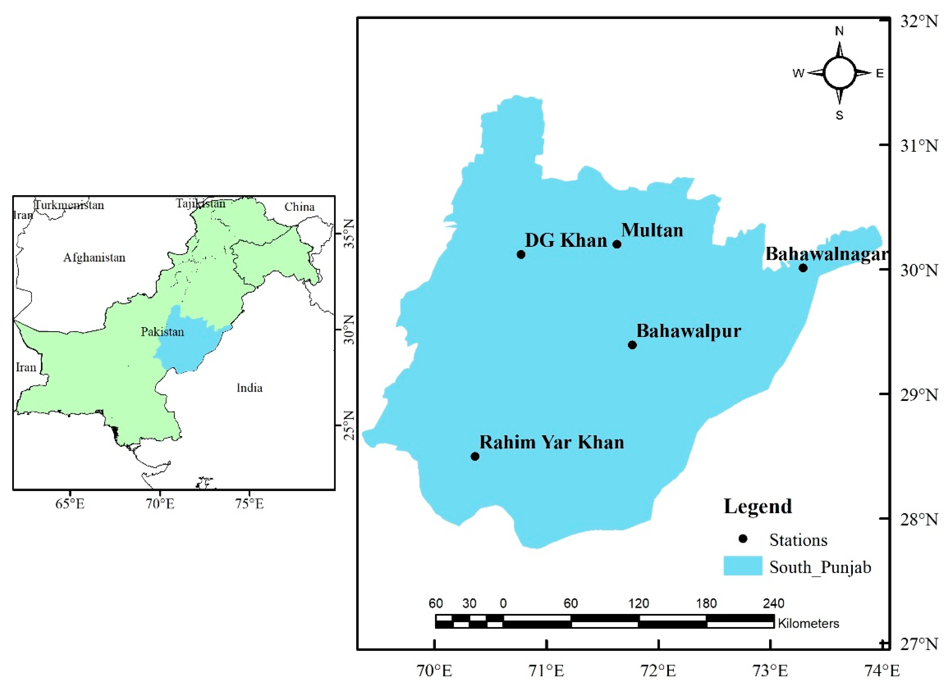
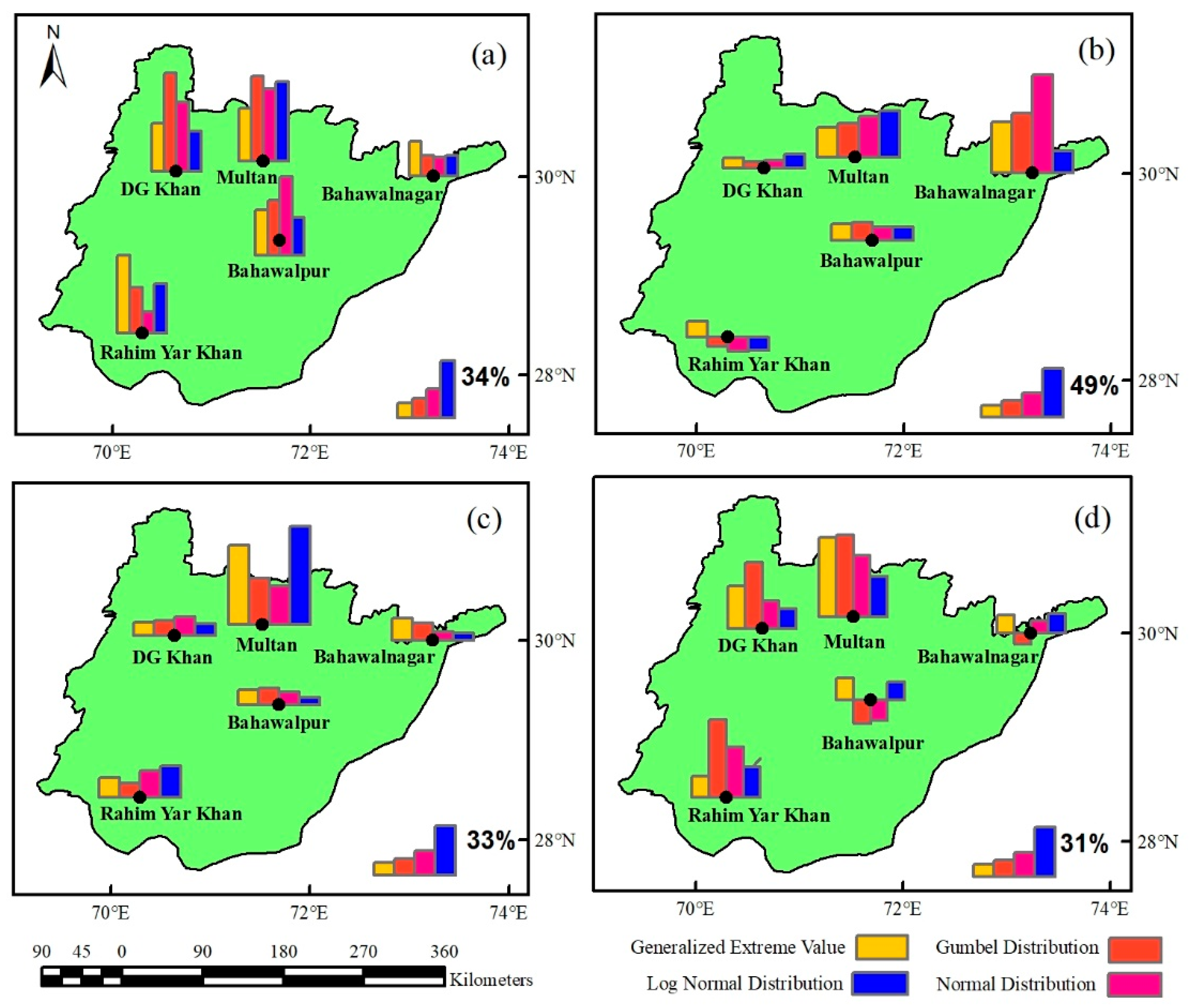
4.1. Selection of Best Probability Distribution Function

The parameters of each distribution were determined by lowering the negative log-likelihood (NLLH) and akaike information criteria (AIC) values. It has been proposed that the distribution with the lowest NLLH and AIC value is the best. Figure 3 provides bar charts of the NLLH and AIC values of each distribution for stationary and nonstationary conditions for yearly maximum precipitation (MP). Each bar chart shows five NLLH values (left) and AIC values (right), one for each of the five stations investigated in this study. The NLLH and AIC statistics of each distribution for nonstationary conditions are frequently lower than those for stationary conditions. This implies that when time was included as a covariate, each distribution fit comparatively well. This demonstrates that the assumption of nonstationarity improves the fit of distributions relatively. In all stationary and nonstationary conditions, NLLH and AIC values for normal distributions were shown to be bigger than NLLH and AIC values for each of the three probability functions. As indicated by bar charts in almost every station, the NLLH and AIC values of the GEV function were lower than those of the other probability functions in most of the precipitation indices under both stationary and nonstationary conditions. For most precipitation indices, the Gumbel distribution has lower NLLH and AIC values than the other two distributions (normal and lognormal) in both stationary and nonstationary conditions. Furthermore, the statistics reveal that the NLLH and AIC values of lognormal distributions are not much higher than those of Gumbel and GEV distributions. Mainly, the GEV distribution will be utilized for future periods since it has the lowest NLLH and AIC values and has traditionally been used more commonly in literature to undertake frequency analysis of extremes because of its tendency to exhibit the best match for tails.

4.2. Impacts of Nonstationarity for the Historic Period (1970–2015)

4.2.1. Yearly Maximum Precipitation (MP)

Figure 4 displays the percentage fluctuations for the 100-year stationary and nonstationary return levels obtained using four probability distributions for yearly MP. With a few notable differences, a visual examination of the maps in Figure 3 demonstrates that all four distributions have proposed analogous consequences for annual MP. There are a number of comparable effect objectives across the stations that are supported to varying degrees by all four distributions. The findings demonstrated that during yearly MP, all four distributions had positive effects on all stations. The level of effects generated by the GEV and lognormal distributions is shown to be greater when compared to the other two distributions. Overall, all of the stations have positive effects from all four probability distributions.

4.2.2. Seasonal MP

The impacts of nonstationarity on seasonal maximum precipitation are presented in Figure 5. Overall, a pattern of nonstationarity impact from all four distributions is seen in the study of seasonal MP. However, a few locations have very minor variations. Seasonal patterns show the importance of seasonality on the return level of the 100-year precipitation over the course of historical time under changing climatic circumstances. While larger return level values are projected throughout the research region in the autumn, the impact type differs between stations in the winter, spring, and summer.
All four distributions have shown more or less comparable effects from nonstationarity during the span of the winter, according to a study of the data for winter MP. Analyzing the four probability distributions, the findings indicate that all of the stations have positive effects. Positive effects’ nonstationarity variability (up to 68%) is seen, especially with the Gumbel distribution over the Multan and DG-Khan stations. Additionally, consequences of nonstationarity (up to 54%) with a normal distribution were seen at the stations in Bahawalpur, Multan, and DG Khan.
During spring, similar nonstationarity impacts have been observed for four probability distributions. There are certain consistent trends in impact types across all stations. Except for GEV, the results show that the three probability distributions have a negative impact on Rahim Yar Khan. All other stations, on the other hand, exhibit a positive impact. The results suggest that adopting GEV has a positive impact (10% to 50%) across all stations. Positive impacts are found with all other probability distributions (6% to 98%) across all stations except Rahim Yar Khan, where negative impacts (9% to 15%) were identified with the three previously mentioned probability distributions.
The results of the nonstationary impact study show that positive impacts were observed during summer MP. The nonstationary impacts of summer MP are very comparable to those of annual MP. The explanation for this is that the majority of the year’s extreme precipitation occurred during the summer season. During the summer MP, all four distributions had a positive impact on all stations, according to the results.
A nonstationary impacts study from all distributions indicated evidence of positive impacts throughout the autumn season. GEV and lognormal distributions, in particular, emphasize this property. However, there were certain locations with a lesser nonstationary impact from the Gumbel and normal distributions. The results demonstrate that utilizing GEV has a positive impact (10 to 65%) across all stations. Positive impacts (up to 63%) were identified across all stations except Bahawalnagar, where negative impacts (9%) were determined using the Gumbel distribution. Moreover, at Bahawalpur, negative impacts (up to 18%) were determined using the Gumbel and normal distributions.

4.3. Impacts of Nonstationarity for Annual Projected Period (2020–2100)

Figure 6 shows the classified maps of the projected models’ (ssp2, ssp5) nonstationary impacts for 100-year return levels using GEV distribution for yearly MP. The estimated time span is divided into two parts: (2020–2060) and (2061–2100). At ssp2 (2020–2060), all projected models show positive nonstationary impacts across all stations. Nonstationary influences are greater in Bahawalnagar and Rahim Yar Khan than in the other three stations. The projected models indicate both types of nonstationary impacts (positive and negative) at ssp2 (2061–2100). Positive effects can be observed in DG-Khan, Multan, and Bahawalpur, where the nonstationary return level of extreme precipitation has increased. Furthermore, except for the GFDL-ESM4 projected model, all of the projected models in Bahawalnagar exhibit negative nonstationary impacts. In Rahim Yar Khan, three of the five projected models exhibit negative nonstationary impacts. Positive nonstationary impacts have been found at all stations during the ssp5 (2020–2060), with the exception of DG-Khan, where three of the five projected models show negative nonstationary impacts. The negative nonstationary impacts dominate the positive nonstationary impacts across all stations in the ssp5 (2061–2100). Except for the GFDL-ESM4 projected model, all other projected models have been found to have negative nonstationary impacts in Rahim Yar Khan, Bahawalpur, and Bahawalnagar. All of the projected models represent a positive impact on the DG-Khan and Multan stations. The nonstationary impacts of the projected model are mostly varying due to variations in the extreme values of the GCMs models.

4.4. Projected Seasonally MP

Table 4 depicts the projected nonstationary impacts (%) for 100-year return levels generated by the GEV distribution at a seasonal scale. During winter, all the projected model shows higher positive nonstationary impacts in Bahawalpur, Rahim Yar Khan, as compared to the other three stations during the ssp2 (2020–2060). The negative nonstationary impacts (up to 6%) were observed in the DG-Khan and Bahawalpur for all the projected models except MPI-ESM1-2hr, MPI-ESM1-2lr, and MRIESM1-0, which show little positive nonstationary impacts. The Positive nonstationary impacts (up to 35%) have been identified for all projected models in Bahawalpur, Bahawalnagar, and DG-Khan during the spring at ssp2 (2020–2060). Except for MPI-ESM1-2HR, MPI-ESM1-2LR, and Mriesm1-0, two of the three forecast models indicated lower extreme precipitation in Multan and Rahim Yar Khan. Positive nonstationary impacts (up to 15%) have been observed in Bahawalpur and DG-Khan during the ssp5 (2020–2060). All of the forecast models revealed positive (up to 4%) and negative (up to 10%) nonstationary impacts at the remaining three stations. Positive nonstationary impacts (up to 35%) have been found for all forecast models across all stations in the ssp2 (2020–2060). During the ssp5 (2020–2060), all stations had positive nonstationary impacts (up to 20%) for all projected models, with the exception of the DG-Khan station, which had two of the five projected models have negative nonstationary impacts (up to 5%). Positive nonstationary impacts were observed throughout all the stations (up to 25%) for all the projected models in the SSP2 (2020–2060). Higher nonstationary return levels (positive nonstationary impacts) of extreme precipitation were found across all stations for the five projected models in the SSP5 (2020–2060), with the exception of Bahawalpur, where one of the five projected models represent positive nonstationary impacts (up to 8%), and the remaining models form negative nonstationary impacts (up to 5%).
During the time period ssp2 (2061–2100), positive nonstationary impacts (up to 35%) were observed in the DG-Khan, Multan, and Rahim Yar Khan generated from the GEV probability distribution using five projected models. A mix type of impacts (positive and negative) was found in the Bahawalnagar and Bahawalpur stations from all the projected models. Two of three projected models, GFDL-ESM4 and MPIESM1-2LR, show positive nonstationary impacts (up to 5%) in the Bahawalnagar and Bahawalpur stations, while the remaining three projected models exhibit negative nonstationary impacts (up to 3%) in the above-mentioned particular stations. Positive nonstationary impacts (up to 15%) are observed in Bahawalnagar and DG-Khan in the ssp2 (2061–2100). The mix of impacts (positive and negative) was observed in the other three stations for all the projected models as shown in Table 5. All of the stations in the ssp5 (2061–2100) demonstrate positive nonstationary impacts (up to 25%), with the exception of Multan, where two of the three models show positive nonstationary impacts (up to 5%), while the remaining three models exhibit negative nonstationary impacts (up to 20%). Positive nonstationary impacts (up to 30%) have been observed at all stations in the ssp2 (2061–2100) except Bahawalnagar and Rahim Yar Khan, where both positive and negative impacts were noted for all forecast models. Negative nonstationary impacts (up to 25%) of severe precipitation were seen in the far future ssp5 (2061–2100) across all stations except DG-Khan and Multan, where higher nonstationary return levels (positive impacts) of extreme precipitation occurred for all projected models. In the SSP2 (2061–2100), all stations formed positive nonstationary impacts except Bahawalnagar and Bahawalpur, where both types of impacts (positive and negative) are found in all the projected models. At ssp5 (2061–2100), the Bahawalpur and Rahim Yar Khan stations have been identified as having higher positive nonstationary impacts (up to 10%), whereas the other three stations have both positive (up to 7%) and negative nonstationary impacts (up to 10%) for all forecast models.

5. Discussion

GEV has the best-fitting properties in both stationary and nonstationary settings out of the four probability distributions. Additionally, GEV offered a better fit for nonstationary distributions compared to stationary distributions. In the research examining nonstationary impacts over the historical and projected eras by Aziz et al. [39], the same conclusions were drawn. This fact was brought about by the use of the same methodology for finding the NLLH using the maximum likelihood estimate. The analysis showed that all distributions exhibit positive nonstationarity impacts at the annual scale; however, it is not necessary for all distributions to have positive nonstationarity effects. For instance, the same four distributions were used for the assessment of nonstationary impacts by Aziz et al. [39] and demonstrated both positive and negative nonstationary impacts at an annual scale. This is because the return period of 30 years used by [39] might be the cause of this inconsistency. Another distinction is that the climate of the study area varies from one place to another or sub-basin to another throughout the world [72]. Hence, the positive impacts of nonstationarity are more likely linked with high quantiles extremes of precipitation [73,74].
Figure 4 and Figure 5 explain the nonstationary impacts raised up to 60% during the historical period for annual and seasonal maximum precipitation. Considering these results in a broader aspect to any region around the globe, it emphasizes the climatic change adoption in the water development sector since more frequent and intensified extreme precipitation events are expected under continuous climate change in the future [30,75,76,77]. Such nonstationary changes in extreme precipitation cause more significant damage or even the failure of existing water conservation facilities. Moreover, enhanced impacts of nonstationary also affect the service life of hydraulic construction projects [78] and other urban infrastructure [79,80] or increase the risk of bridge and highway damage or even failure [81].
Furthermore, nonstationary conditions lead to an increase or decrease in the return level of extreme precipitation that may have a positive or negative nonstationary impact [39]. Since the number of hot and rainy days, land use patterns, and soil moisture levels fluctuate on a seasonal basis, the return levels of extreme precipitation increase in a complex way [30]. According to the current study, the return level of extreme precipitation increased over the winter season, indicating that there were more instances of extreme precipitation.
The results also showed that the return level of extreme precipitation under nonstationary conditions is inconsistent for both the historical and future periods. The complexity of the climate system under nonstationary conditions is explained by these tendencies in these results [73]. Furthermore, the historical data in time-dependent variations of the return level for a certain return period would not remain true for a longer length of time in the future. Nonstationary impacts in terms of nonstationary return level for extreme precipitation may increase in the twenty-first century. Moreover, Aziz et al., [61] showed more consistent nonstationarity effects for temperature extremes at seasonal and annual scales from historical to future times. The investigation of historic-based analysis may only be helpful for short-run strategy and decision-making, while analysis based upon both historical and projected data may be more suitable for long-term strategy planning.

6. Conclusions

In this study, the return level of extreme precipitation was estimated under nonstationary and stationary assumptions to evaluate nonstationary impacts for historical and projected extreme precipitation. The conclusions of the study are as follows:
-
Although GEV (initially having three components) is a widely used probability distribution. The findings of this study reveal that alternative distributions are also capable of comparing nonstationary impacts. The less complicated distributions (having two parameters) might prove advantageous at a particular station.
-
The increase in the return level (magnitude) of extreme precipitation in winter and spring showed causes of flood events, and the reduction in return level of extreme precipitation in summer and autumn may cause less water availability.
-
The projected increase in nonstationarity impacts (up to 50%) distinguished the climate change in the region and emphasized the nonstationarity in the design of hydraulic structures (Reservoirs, Barrages, and others).
No doubt, nonstationary exists in the data series of hydro-meteorological parameters. This study was conducted in a flat area that is arid where a nonstationary impact of up to 60% is observed during the historical period for annual and seasonal maximum precipitation. The findings emphasize the water development sector to adopt the climatic change in terms of nonstationarity impacts. However, the results based on historical data analysis can also be evaluated with other parameter estimation methods of probability distributions, such as linear moments (L-moments). Moreover, the results based on projected data by GCM show uncertainties because, in general, it suffers from great deficiencies and errors, being indicative in nature. The CMIP6 precipitation projections are quite uncertain, thus requiring further assessment and correction [82,83].

Author Contributions

All authors were involved in the intellectual elements of this paper. M.U.K. and M.I. designed the research. M.U.K. and R.A. conducted the research and wrote the manuscript. M.W.I., M.M. and M.A.U.R.T. helped in the analysis. All authors have read and agreed to the published version of the manuscript.

Funding

This research received no external funding.

Data Availability Statement

The data used in this study, including observed precipitation and CMIP6 GCM model data, which is freely available and can be accessed from the websites given in the data section of the manuscript. However, the observed data is the property of the Pakistan Meteorological Department (PMD) and can be requested via official channels.

Acknowledgments

The authors are grateful to the Centre of Excellence in Water Resource Engineering, UET, Lahore, and College of Engineering, IT and Environment, Charles Darwin University, Australia, for support in conducting this study. The authors are also thankful to the Pakistan Meteorological Department (PMD) for providing the observed meteorological data used in the study.

Conflicts of Interest

The authors declare no conflict of interest.

References

  1. IPCC. Summary for Policymakers. In Climate Change 2021: The Physical Science Basis; Contribution of Working Group I to the Sixth Assessment Report of the Intergovernmental Panel on Climate Change; Masson-Delmotte, V., Zhai, P., Pirani, A., Connors, S.L., Péan, C., Berger, S., Caud, N., Chen, Y., Goldfarb, L., Gomis, M.I., et al., Eds.; Cambridge University Press: Cambridge, UK, 2021. [Google Scholar]
  2. Mishra, A.K.; Singh, V.P. Changes in extreme precipitation in Texas. J. Geophys. Res. 2010, 15, D14106. [Google Scholar] [CrossRef]
  3. López, J.; Francés, F. Nonstationary flood frequency analysis in continental Spanish rivers, using climate and reservoir indices as external covariates. Hydrol. Earth Syst. Sci. 2013, 17, 3189–3203. [Google Scholar] [CrossRef]
  4. Stedinger, J.R.; Vogel, R.; Foufoula-Georgiou, E. Frequency analysis of extreme events. Handb. Hydrol. 1993, 18, 68. [Google Scholar]
  5. Salas, J. Analysis and Modeling of Hydrologic Time Series in Hand Book of Hydrology; Maidment, D.R., Ed.; McGraw Hill Book Co.: New York, NY, USA, 1993. [Google Scholar]
  6. Council, N.R. Decade-to-Century-Scale Climate Variability and Change: A Science Strategy; National Academies Press: Washington, DC, USA, 1998. [Google Scholar]
  7. Norrant, C.; Douguédroit, A. Monthly and daily precipitation trends in the Mediterranean (1950–2000). Theor. Appl. Climatol. 2006, 83, 89–106. [Google Scholar] [CrossRef]
  8. Mudelsee, M.; Börngen, M.; Tetzlaff, G.; Grünewald, U. No upward trends in the occurrence of extreme floods in central Europe. Nature 2003, 425, 166–169. [Google Scholar] [CrossRef]
  9. Douglas, E.; Vogel, R.; Kroll, C. Trends in floods and low flows in the United States: Impact of spatial correlation. J. Hydrol. 2000, 240, 90–105. [Google Scholar] [CrossRef]
  10. Franks, S.W. Identification of a change in climate state using regional flood data. Hydrol. Earth Syst. Sci. 2002, 6, 11–16. [Google Scholar] [CrossRef]
  11. Milly, P.C.; Dunne, K.A.; Vecchia, A.V. Global pattern of trends in streamflow and water availability in a changing climate. Nature 2005, 438, 347–350. [Google Scholar] [CrossRef]
  12. Villarini, G.; Serinaldi, F.; Smith, J.A.; Krajewski, W.F. On the stationarity of annual flood peaks in the continental united states during the 20th century. Water Resour. Res. 2009, 45, W08417. [Google Scholar] [CrossRef]
  13. Wilson, D.; Hisdal, H.; Lawrence, D. Has streamflow changed in the nordic countries?—Recent trends and comparisons to hydrological projections. J. Hydrol. 2010, 394, 334–346. [Google Scholar] [CrossRef]
  14. Villarini, G.; Smith, J.A.; Serinaldi, F.; Bales, J.; Bates, P.D.; Krajewski, W.F. Flood frequency analysis for nonstationary annual peak records in an urban drainage basin. Adv. Water Resour. 2009, 32, 1255–1266. [Google Scholar] [CrossRef]
  15. Vogel, R.M.; Yaindl, C.; Walter, M. Nonstationarity: Flood magnification and recurrence reduction factors in the United States. J. Am. Water Resour. Assoc. 2011, 47, 464–474. [Google Scholar] [CrossRef]
  16. Hejazi, M.I.; Markus, M. Impacts of urbanization and climate variability on floods in northeastern Illinois. J. Hydrol. Eng. 2009, 14, 606–616. [Google Scholar] [CrossRef]
  17. Milly, P.C.; Betancourt, J.; Falkenmark, M.; Hirsch, R.M.; Kundzewicz, Z.W.; Lettenmaier, D.P.; Stouffer, R.J. Stationarity is dead: Whither water management? Science 2008, 319, 573–574. [Google Scholar] [CrossRef] [PubMed]
  18. Nawaz, Z.; Li, X.; Chen, Y.; Guo, Y.; Wang, X.; Nawaz, N. Temporal and spatial characteristics of precipitation and temperature in Punjab, Pakistan. Water 2019, 11, 1916. [Google Scholar] [CrossRef]
  19. Jain, S.K.; Kumar, V.; Saharia, M. Analysis of rainfall and temperature trends in northeast India. Int. J. Climatol. 2013, 33, 968–978. [Google Scholar] [CrossRef]
  20. Beck, H.E.; Pan, M.; Roy, T.; Weedon, G.P.; Pappenberger, F.; van Dijk, A.I.J.M.; Huffman, G.J.; Adler, R.F.; Wood, E.F. Daily evaluation of 26 precipitation datasets using Stage-IV gauge-radar data for the CONUS. Hydrol. Earth Syst. Sci. 2019, 23, 207–224. [Google Scholar] [CrossRef]
  21. Hamdi, M.R.; Abu-Allaban, M.; Elshaieb, A.; Jaber, M.; Momani, N.M. Climate change in Jordan: A comprehensive examination approach. Am. J. Environ. Sci. 2009, 5, 740–750. [Google Scholar] [CrossRef]
  22. Matti, C.; Pauling, A.; Küttel, M.; Wanner, H. Winter precipitation trends for two selected European regions over the last 500 years and their possible dynamical background. Theor. Appl. Climatol. 2009, 95, 9–26. [Google Scholar] [CrossRef]
  23. Singh, P.; Kumar, V.; Thomas, T.; Arora, M. Basin-wide assessment of temperature trends in northwest and central India/Estimation par bassin versant de tendances de température au nord-ouest et au centre de l’Inde. Hydrol. Sci. J. 2008, 53, 421–433. [Google Scholar] [CrossRef]
  24. De la Casa, A.; Nasello, O. Breakpoints in annual rainfall trends in Córdoba, Argentina. Atmos. Res. 2010, 95, 419–427. [Google Scholar] [CrossRef]
  25. Gleick, P.H. Climate change, hydrology, and water resources. Rev. Geophys. 1989, 27, 329–344. [Google Scholar] [CrossRef]
  26. Feng, S.; Hu, Q.; Qian, W. Quality control of daily meteorological data in China, 1951–2000: A new dataset. Int. J. Climatol. A J. R. Meteorol. Soc. 2004, 24, 853–870. [Google Scholar] [CrossRef]
  27. Jiang, S.; Ren, L.; Hong, Y.; Yong, B.; Yang, X.; Yuan, F.; Ma, M. Comprehensive evaluation of multi-satellite precipitation products with a dense rain gauge network and optimally merging their simulated hydrological flows using the Bayesian model averaging method. J. Hydrol. 2012, 452, 213–225. [Google Scholar] [CrossRef]
  28. Liu, X.; Yang, T.; Hsu, K.; Liu, C.; Sorooshian, S. Evaluating the streamflow simulation capability of PERSIANN-CDR daily rainfall products in two river basins on the Tibetan Plateau. Hydrol. Earth Syst. Sci. 2017, 21, 169–181. [Google Scholar] [CrossRef]
  29. Fischer, E.; Knutti, R. Anthropogenic contribution to global occurrence of heavy-precipitation and high-temperature extremes. Nat. Clim. Chang. 2015, 5, 560–564. [Google Scholar] [CrossRef]
  30. Donat, M.; Lowry, A.; Alexander, L.; O’Gorman, P.A.; Maher, N. More extreme precipitation in the world’s dry and wet regions. Nat. Clim. Chang. 2016, 6, 508–513. [Google Scholar] [CrossRef]
  31. IPCC. Managing the Risks of Extreme Events and Disasters to Advance Climate Change Adaptation; A Special Report of Working Groups I and II of the Intergovernmental Panel on Climate, Change; Field, C.B., Barros, V., Stocker, T.F., Qin, D., Dokken, D.J., Ebi, K.L., Mastrandrea, M.D., Mach, K.J., Plattner, G.-K., Allen, S.K., et al., Eds.; Cambridge University Press: Cambridge, UK; New York, NY, USA, 2012; 582p. [Google Scholar]
  32. Schellnhuber, H.J.; Hare, B.; Serdeczny, O. Turn Down the Heat: Climate Extremes, Regional Impacts, and the Case for Resilience; A Report for the World Bank by the Potsdam Institute for Climate Impact Research and Climate Analytics; World Bank: Washington, DC, USA, 2013. [Google Scholar]
  33. Eckstein, D.; Hutfils, M.-L.; Winges, M. Global Climate Risk Index; Germanwatch: Berlin, Germany, 2019. [Google Scholar]
  34. Khan, F.; Ali, S.; Ullah, H.; Muhammad, S. Twenty-first century climate extremes’ projections and their spatio-temporal trend analysis over Pakistan. J. Hydrol. Reg. Stud. 2023, 45, 101295. [Google Scholar] [CrossRef]
  35. Ahmad, I.; Tang, D.; Wang, T.; Wang, M.; Wagan, B. Precipitation Trends over Time Using Mann-Kendall and Spearman’s rho Tests in Swat River Basin, Pakistan. Adv. Meteorol. 2015, 2015, 431860. [Google Scholar] [CrossRef]
  36. Khattak, M.S.; Reman, N.U.; Sharif, M.; Khan, M.A. Analysis of streamflow data for trend detection on major rivers of the Indus Basin. J. Himal. Earth Sci. 2015, 48, 87. [Google Scholar]
  37. Katz, R.W.; Parlange, M.B.; Naveau, P. Statistics of extremes in hydrology. Adv. Water Resour. 2002, 25, 1287–1304. [Google Scholar] [CrossRef]
  38. Vogel, R.M.; Read, L.K. Reliability, return periods and risk under nonstationarity. Water Resour. Res. 2015, 51, 6381–6398. [Google Scholar] [CrossRef]
  39. Aziz, R.; Yucel, I.; Yozgatligil, C. Nonstationarity impacts on frequency analysis of yearly and seasonal extreme precipitation in Turkey. Theor. Appl. Climatol. 2021, 143, 1213–1226. [Google Scholar] [CrossRef]
  40. Sertac, O. Nonstationary Investigation of Extreme Rainfall. Civ. Eng. J. 2021, 7, 1620–1633. [Google Scholar]
  41. Nashwan, M.S.; Tarmizi, I.; Kamal, A. Nonstationary Analysis of extreme Rainfall in Peninsular Malaysia. J. Sust. Sci. Mgmt. 2019, 14, 17–34. [Google Scholar]
  42. Mirza, M.M.Q. Climate change and extreme weather events: Can developing countries adapt? Clim. Policy 2003, 3, 233–248. [Google Scholar] [CrossRef]
  43. Linnenluecke, M.K.; Stathakis, A.; Griffiths, A. Firm relocation as adaptive response to climate change and weather extremes. Glob. Environ. Chang. 2011, 21, 123–133. [Google Scholar] [CrossRef]
  44. Chen, X.C.; Xu, Y.; Xu, C.H.; Yao, Y. Assessment of precipitation simulations in China by CMIP5 multi-models. Clim. Chang. Res. 2014, 10, 217–225. [Google Scholar]
  45. Ta, Z.; Yu, Y.; Sun, L.; Chen, X.; Mu, G.; Yu, R. Assessment of Precipitation Simulations in Central Asia by CMIP5 Climate Models. Water 2018, 10, 1516. [Google Scholar] [CrossRef]
  46. Huang, X.H.; Yue, Q.; Zhang, M. Future precipitation change in the Belt and Road Region under Representative Concentration Pathway Scenarios. J. Yangtze River Sci. Res. Inst. 2020, 37, 53–60. [Google Scholar]
  47. Salman, S.A.; Nashwan, M.S.; Ismail, T.; Shahid, S. Selection of CMIP5 general circulation model outputs of precipitation for peninsular Malaysia. Hydrol. Res. 2020, 51, 781–798. [Google Scholar] [CrossRef]
  48. Zhang, Q.M.; Wang, R.; Jiang, T.; Chen, S.S. Projection of extreme precipitation in the Hanjiang River basin under different RCP scenarios. Clim. Chang. Res. 2020, 16, 276–286. [Google Scholar]
  49. Huang, J.L.; Wang, Y.J.; Su, B.D.; Zhai, J.Q. Future climate change and its impact on runoff in the upper reaches of the Yangtze River under RCP4.5 scenario. Meteor Mon. 2016, 42, 614–620. [Google Scholar]
  50. Montroull, N.B.; Saurral, R.I.; Camilloni, I.A. Hydrological impacts in La Plata basin under 1.5, 2 and 3 °C global warming above the pre-industrial level. Int. J. Climatol. 2018, 38, 3355–3368. [Google Scholar] [CrossRef]
  51. Ashiq, M.W.; Zhao, C.; Ni, J.; Akhtar, M. GIS-based high-resolution spatial interpolation of precipitation in mountain–plain areas of Upper Pakistan for regional climate change impact studies. Theor. Appl. Climatol. 2010, 99, 239. [Google Scholar] [CrossRef]
  52. Ali, A.F.; Xiao, C.-D.; Zhang, X.-P.; Adnan, M.; Iqbal, M.; Khan, G. Projection of future streamflow of the Hunza River Basin, Karakoram Range (Pakistan) using HBV hydrological model. J. Mt. Sci. 2018, 15, 2218–2235. [Google Scholar] [CrossRef]
  53. Syed, Z.; Ahmad, S.; Dahri, Z.H.; Azmat, M.; Shoaib, M.; Inam, A.; Qamar, M.U.; Hussain, S.Z.; Ahmad, S. Hydroclimatology of the Chitral River in the Indus Basin under Changing Climate. Atmosphere 2022, 13, 295. [Google Scholar] [CrossRef]
  54. Waseem, M.; Ajmal, M.; Ahmad, I.; Khan, N.M.; Azam, M.; Sarwar, M.K. Projected drought pattern under climate change scenario using multivariate analysis. Arab. J. Geosci. 2021, 14, 544. [Google Scholar] [CrossRef]
  55. Masood, M.U.; Khan, N.M.; Haider, S.; Anjum, M.N.; Chen, X.; Gulakhmadov, A.; Iqbal, M.; Ali, Z.; Liu, T. Appraisal of Land Cover and Climate Change Impacts on Water Resources: A Case Study of Mohmand Dam Catchment, Pakistan. Water 2023, 15, 1313. [Google Scholar] [CrossRef]
  56. Diaz-Nieto, J.; Wilby, R.L. A comparison of statistical downscaling and climate change factor methods: Impacts on low flows in the River Thames, United Kingdom. Clim. Chang. 2005, 69, 245–268. [Google Scholar] [CrossRef]
  57. Mann, H.B.; Whitney, D.R. On a test of whether one of two random variables is stochastically larger than the other. Ann. Math. Stat. 1947, 18, 50.e60. [Google Scholar] [CrossRef]
  58. Fawad, M.; Yan, T.; Chen, L.; Huang, K.; Singh, V.P. Multiparameter probability distributions for at-site frequency analysis of annual maximum wind speed with L-Moments for parameter estimation. Energy 2019, 181, 724–737. [Google Scholar] [CrossRef]
  59. Iqbal, M.; Wen, J.; Wang, X.; Lan, Y.; Tian, H.; Anjum, M.N.; Adnan, M. Assessment of Air Temperature Trends in the Source Region of Yellow River and Its Sub-Basins, China. Asia-Pac. J. Atmos. Sci. 2017, 54, 111–123. [Google Scholar] [CrossRef]
  60. Aziz, R.; Yücel, I.; Yozgatlıgil, C. Nonstationarity impacts on frequency analysis of yearly and seasonal extreme temperature in Turkey. Atmos. Res. 2020, 238, 104875. [Google Scholar] [CrossRef]
  61. Seo, J.; Sangdan, K. Uncertainty of Rate of change in Korean Future Rainfall Extremes Using Non-Stationary GEV Model. Atmos. J. 2021, 12, 227. [Google Scholar] [CrossRef]
  62. Gellens, D. Combining regional approach and data extension procedure for assessing GEV distribution of extreme precipitation in Belgium. J. Hydrol. 2002, 268, 113–126. [Google Scholar] [CrossRef]
  63. Gründemann, G. Extreme precipitation return levels for multiple durations on a global scale. J. Hydrol. 2022, 621, 129558. [Google Scholar] [CrossRef]
  64. Kang, D. Determination of extreme wind values using the Gumbel distribution. Energy 2015, 86, 51–58. [Google Scholar] [CrossRef]
  65. Salas, J.D.; Obeysekera, J. Revisiting the concepts of return period and risk for nonstationary hydrologic extreme events. J. Hydrol. Eng. 2014, 19, 554–568. [Google Scholar] [CrossRef]
  66. Katz, R.W. Chapter 2, Extremes in a changing climate: Detection, analysis and uncertainty. In Statistical Methods for Nonstationary Extremes; Kouchak, A., Easterling, D., Hsu, K., Eds.; Springer: New York, NY, USA, 2013; Volume 65. [Google Scholar]
  67. Coles, S. An Introduction to Statistical Modeling of Extreme Values; Springer Series in Statistics; Springer: London, UK, 2021. [Google Scholar]
  68. Cannon, A.J. GEVcdn: An R package for nonstationary extreme value analysis by generalized extreme value conditional density estimation network. Comput. Geosci. 2011, 37, 1532L–1533L. [Google Scholar] [CrossRef]
  69. Heffernan, J.; Stephenson, A. Ismev: An Introduction to Statistical Modeling of Extreme Values. R Package Version 1.39, Original S Functions Written by Janet E. Heffernan with R port and R Documentation Provided by Alec G. Stephenson. 2012. Available online: https://CRAN.R-project.org/package=ismev (accessed on 3 March 2023).
  70. Gilleland, E.; Katz, R. New software to analyze how extremes change over time. EOS Trans. Am. Geophys. Union 2011, 92, 13–14. [Google Scholar] [CrossRef]
  71. Gilleland, E. extRemes: Extreme Value Analysis. R Package Version 2.0-8. 2016. Available online: https://CRAN.R-project.org/package=extRemes (accessed on 3 March 2023).
  72. Trenberth, K.E.; Jones, P.D.; Ambenje, P.; Bojariu, R.; Easterling, D.; Klein, T.A.; Parker, D.; Rahimzadeh, F.; Renwick, J.A.; Rusticucci, M.; et al. Observations: Surface and atmospheric climate change. In Climate Change 2007: The Physical Science Basis. Contribution of Working Group I to the Fourth Assessment Report of the Intergovernmental Panel on Climate Change; Solomon, S., Qin, D., Manning, M., Marquis, M., Averyt, K., Tignor, M.M.B., Miller, H.L., Jr., Chen, Z., Eds.; Cambridge University Press: Cambridge, UK, 2007; pp. 235–336. [Google Scholar]
  73. IPCC. Climate Change 2007: Impacts, Adaptation, and Vulnerability; Parry, M.L., Canziani, O.F., Palutikof, J.P., van der Linden, P.J., Hanson, C.E., Eds.; Cambridge University Press: Cambridge, UK, 2007. [Google Scholar]
  74. Xiao, M.; Zhang, Q.; Singh, V.P. Spatiotemporal variations of extreme precipitation regimes during 1961–2010 and possible teleconnections with climate indices across China. Int. J. Climatol. 2017, 37, 468–479. [Google Scholar] [CrossRef]
  75. Papalexiou, S.M.; Montanari, A. Global and regional increase of precipitation extremes under global warming. Water Resour. Res. 2019, 55, 4901–4914. [Google Scholar] [CrossRef]
  76. Huang, H.F.; Cui, H.J.; Ge, Q.S. Assessment of potential risks induced by increasing extreme precipitation under climate change. Nat. Hazards 2021, 108, 2059–2079. [Google Scholar] [CrossRef]
  77. Valdez, B.; Schorr, M.; Quintero, M.; García, R.; Rosas, N. Effect of climate change on durability of engineering materials in hydraulic infrastructure: An overview. Corros. Eng. Sci. Technol. 2010, 45, 34–41. [Google Scholar] [CrossRef]
  78. Mailhot, A.; Duchesne, S. Design criteria of urban drainage infrastructures under climate change. J. Water Resour. Plann. Manag. 2010, 136, 201–208. [Google Scholar] [CrossRef]
  79. Al-Ghadi, M.S.; Mohtar, W.H.M.W.; Razali, S.F.M.; El-Shafie, A. The practical influence of climate change on the performance of road stormwater drainage infrastructure. J. Eng. 2020, 2020, 8582659. [Google Scholar] [CrossRef]
  80. Akhtar, A.A.; Esquivel, A.; Sharma, M.; Tandon, V. Understanding Climate Change Impact on Highway Hydraulic Design Procedures; Southern Plains Transportation Center: Norman, OK, USA, 2018. [Google Scholar]
  81. Akhter, A.A. Assessment of Climate Change Impact on Hydraulic Design Procedures of Bridges. Master’s Thesis, The University of Texas at El Paso, El Paso, TX, USA, 2018. [Google Scholar]
  82. Pan, H.; Jin, Y.; Zhu, X. Comparison of Projections of Precipitation over Yangtze River Basin of China by Different Climate Models. Water 2022, 14, 1888. [Google Scholar] [CrossRef]
  83. Wang, H.-M.; Chen, J.; Xu, C.-Y.; Zhang, J.; Chen, H. A framework to quantify the uncertainty contribution of GCMs over multiple sources in hydrological impacts of climate change. Earth′s Future 2020, 8, e2020EF001602. [Google Scholar] [CrossRef]
Figure 1. Location Map of South Punjab with Climatic Stations.
Water 15 03958 g001
Figure 2. Schematic flowchart of adopted methodology for the study.
Water 15 03958 g002
Figure 3. Comparison of NLLH (left) and AIC (right) values of probability distributions for annual maximum precipitation of historical data under stationary and nonstationary assumptions.
Water 15 03958 g003
Figure 4. Nonstationary impacts at 100-year return levels for annual maximum precipitation using different probability distributions. The impacts at a particular station are examined with reference to the given maximum scale bar in legends.
Water 15 03958 g004
Figure 5. Classified maps of seasonal nonstationary impacts for 100-year return levels using different probability distributions (a) Winter, (b) Spring, (c) Summer, and (d) Autumn. The nonstationary impacts at a particular station are examined with reference to the given maximum scale bar in legends.
Water 15 03958 g005
Figure 6. Classified projected annual maps of nonstationary impacts for 100-year return levels using GEV probability distribution (a) ssp2 (2020–2060), (b) ssp2 (2061–2100), (c) ssp5 (2020–2060), (d) ssp5 (2061–2100). The nonstationary impacts at a particular station are examined with reference to the given maximum scale bar in legends.
Water 15 03958 g006
Table 1. Selected CMIP6 Model for Precipitation Data of SSP2 and SSP 5 Scenarios.
Institution IDModel NameResolution (Long, Lat)
NOAA-GFDLGFDL1.3° × 1.0°
MIROCMIROC61.4° × 1.4°
MPIESM1-2HRMPI-ESM1-2HR0.9° × 0.9°
MPI-MMPIESM1-2LR1.9° × 1.9°
MRIESM2-0MRIESM2-01.12° × 1.12°
Table 2. Mean annual precipitation statistics of the study area.
StationsLatitudeLongitudeElevationMeanSTDCvCsCk
Bahawalnagar29°20′73°51′161.05254.34126.550.500.42−0.59
Bahawalpur29°20′71°47′110177.58119.340.671.674.08
Multan30°12′71°26′121.95197.48104.590.530.460.90
Rahim Yar Khan28°26′70°19′82.93112.3578.700.700.860.39
DG Khan30°03′70°38′148.1170.12109.830.650.850.56
Table 3. p value (two-tailed) for analyzed series by Mann–Whitney U Test.
StationAnnualWinterSpringSummer
Bahawalnagar0.090.150.650.15
Bahawalpur0.880.030.581.00
DG Khan0.790.710.840.58
Multan0.380.170.490.38
Rahim Yar Khan0.300.20.760.31
Table 4. Projected nonstationary impacts (%) for 100-year return levels using GEV probability distribution during 2020–2060.
StationGCM ModelGFDLMIROC6MPI-ESM1-2HRMPI-ESM1-2LRMRISEM1-0
SeasonSSP2SSP5SSP2SSP5SSP2SSP5SSP2SSP5SSP2SSP5
BahawalnagarWinter25.8−5.323.4−3.522.71.921.51.824.1−4.4
Spring33.02.430.3−2.930.2−2.629.4−3.831.32.0
Summer33.39.531.12.532.73.032.32.632.42.8
Autumn13.93.414.011.316.15.213.712.914.56.9
BahawalpurWinter−4.012.6−9.913.52.613.22.112.6−3.313.8
Spring23.57.820.85.220.73.019.95.021.85.4
Summer3.73.24.12.72.72.13.73.62.93.4
Autumn5.69.97.5−5.210.4−3.18.3−7.14.4−3.7
DG KhanWinter5.616.05.215.95.0−5.44.7−4.55.2−6.4
Spring−11.33.3−15.3−11.03.52.92.5−10.63.9−11.3
Summer3.91.53.85.63.37.33.76.52.68.2
Autumn8.717.18.313.28.011.112.512.88.313.8
MultanWinter−2.512.6−1.911.82.411.5−6.510.83.212.2
Spring19.25.317.615.317.514.912.414.518.215.4
Summer2.2−6.42.52.43.92.55.4−5.52.03.4
Autumn12.88.414.612.916.812.411.511.719.44.3
Rahim Yar khanWinter11.12.59.84.39.4−4.28.8−5.910.1−4.5
Spring−10.53.7−4.22.5−6.3−9.93.9−9.24.1−11.2
Summer12.915.513.25.813.58.412.49.511.210.3
Autumn6.96.46.58.88.55.510.29.06.69.8
Table 5. Projected nonstationary impacts (%) for 100-year return levels using GEV probability distribution during 2061–2100.
StationGCM ModelGFDLMIROC6MPI-ESM1-2HRMPI ESM1-2LRMRISEM1-0
SeasonSSP2SSP5SSP2SSP5SSP2SSP5SSP2SSP5SSP2SSP5
BahawalnagarWinter3.87.0−2.9−9.7−3.5−10.67.88.3−4.5−10.3
Spring12.62.312.27.912.16.18.96.910.18.4
Summer2.18.0−11.2−11.7−9.5−13.3−9.4−11.0−10.5−12.6
Autumn2.83.9−7.53.1−5.23.3−7.53.22.33.5
BahawalpurWinter4.67.1−4.84.1−4.66.82.74.8−4.66.9
Spring2.23.1−1.84.0−2.85.23.84.84.55.8
Summer4.14.73.3−12.94.2−14.34.3−11.23.9−9.3
Autumn3.72.6−5.5−6.5−12.5−2.5−7.52.2−10.8−1.5
DG KhanWinter25.411.627.28.526.59.827.18.626.79.1
Spring3.55.0−13.4−14.9−12.2−15.15.37.5−12.2−14.6
Summer30.117.528.422.427.516.825.512.622.524.1
Autumn12.62.06.4−1.67.9−1.39.21.713.9−1.9
MultanWinter18.97.719.55.918.36.218.96.118.36.5
Spring5.518.812.212.79.413.115.212.87.412.7
Summer4.29.43.214.54.514.94.913.95.917.4
Autumn11.25.17.5−3.39.9−7.213.53.28.3−8.5
Rahim Yar khanWinter1.51.412.62.615.53.211.73.69.54.6
Spring5.05.64.98.8−4.78.8−4.98.7−7.79.0
Summer3.56.0−10.5−11.1−10.4−13.78.4−9.4−2.8−10.3
Autumn2.76.35.15.18.83.311.64.74.85.0
Disclaimer/Publisher’s Note: The statements, opinions and data contained in all publications are solely those of the individual author(s) and contributor(s) and not of MDPI and/or the editor(s). MDPI and/or the editor(s) disclaim responsibility for any injury to people or property resulting from any ideas, methods, instructions or products referred to in the content.

