1. Introduction
Hydropower stations are of great significance to flood control and drought resistance, water and energy security, and the comprehensive utilization and management of water resources. With the increase in the number of hydropower stations, the efficiency promotion of existing hydropower stations based on the premise of safe operation has been a growing concern in recent years. For most hydropower stations, the precise control of water levels is at the core of dispatching and operating hydropower stations and the base of safe and economic operation and management. Therefore, the accurate prediction of water levels has gained increasing attention as it provides valuable support for the precise operation of hydropower stations. In particular, the prediction of the tail water level (TWL) is of great importance for the economic operation and management of a power station. The TWL directly impacts the power generation efficiency of a hydropower station [
1]. Hence, accurate prediction of the TWL can significantly contribute to the operation planning of a hydropower station.
Current water level prediction methods can be divided into physics-driven models and data-driven models. Physical-driven models work by solving equations based on hydrodynamics equations or water balance equations [
2]. The hydrodynamic model mainly uses the Saint-Venant equations and boundary condition data to calculate the river network. In order to improve the calculation feasibility, many assumptions are added, resulting in low calculation accuracy. With the deepening of people’s understanding of the hydrodynamic mechanism and the development of computer technology, the hydrodynamic model is constantly improving, but its computational complexity is getting higher and higher [
3]. However, it is still difficult to describe the physical mechanism accurately with equations when there is a propagation time problem between variables of the hydropower station or in more complex, special cases. Therefore, many hydropower stations use the combination of the physics-driven model and the statistical method in practical application to improve the calculation accuracy and efficiency. Through statistical calculations of historical operation data, the empirical curve describing the correlation of variables is summarized to calculate the variables that cannot be accurately described by the equation, such as the water level–storage capacity curve and the TWL–outbound flow rate curve [
4].
A data-driven model refers to a model that summarizes patterns from historical operational data and applies them to future data forecasting [
5]. The empirical curve is a simple data-driven model that summarizes the corresponding relationship between the combination of target variables and feature variables. A target variable can be calculated by finding a similar situation in the empirical curve table. However, the simple data-driven model cannot handle nonlinear relationships, which are ubiquitous in the research of water level prediction. Therefore, machine learning, such as artificial neural network (ANN), random forest (RF), and support vector machine (SVM), which can be immune to these limitations, is widely used in water level prediction research [
6,
7,
8,
9]. But, the machine learning methods still cannot adapt to the temporal dependencies in the water level prediction problem. The recurrent neural network (RNN), as a kind of deep learning model, can excavate temporal dependencies to improve the forecasting accuracy. As an improved RNN model, the LSTM model can effectively slow down the gradient disappearance or explosion that may occur in long sequence problems, which has attracted the attention of many scholars [
10,
11,
12]. Shuofeng, L. [
12] focus on the precipitation-only water level forecasting problem by using an LSTM-based hybrid model and try predicting the future water levels of all of the rivers in Japan by using simulated precipitation data from the database for policy decision making for future climate change (d4PDF). Zhang, Z. [
13] use the maximal information coefficient and feature combination to select feature inputs, construct a CNN-LSTM neural network to predict the downstream water level of a reservoir, and then compare the method with four state-of-the-art prediction methods; they find that the designed method is also very competitive.
While there are numerous water level prediction methods available, the majority of them mainly focus on longer time scales, typically exceeding one day [
14,
15], and they primarily consider upstream water levels [
16,
17]. There are limited studies that specifically address tail water level (TWL) prediction and consider the downstream backwater effect, despite its obvious significance. The Xiangjiaba hydropower station (XJB), as China’s third largest hydropower station and the fifth largest globally, plays a vital role in power generation, shipping, and ecological benefits. The downstream tributary’s backwater effect on the XJB’s TWL can reach approximately 3 m, significantly impacting the accuracy of tail water level predictions, thus posing a major operational challenge. Hence, the establishment of a TWL prediction model that accounts for the backwater effect becomes crucial in achieving accurate predictions under such conditions.
The structure of the paper is as follows.
Section 2 will provide an overview of the research area and the research methodology employed. In
Section 3, the research process will be analyzed.
Section 4 will present the analysis of the model prediction results. Finally, the paper will conclude with a summary of the findings.
3. Analysis of Backwater Effect
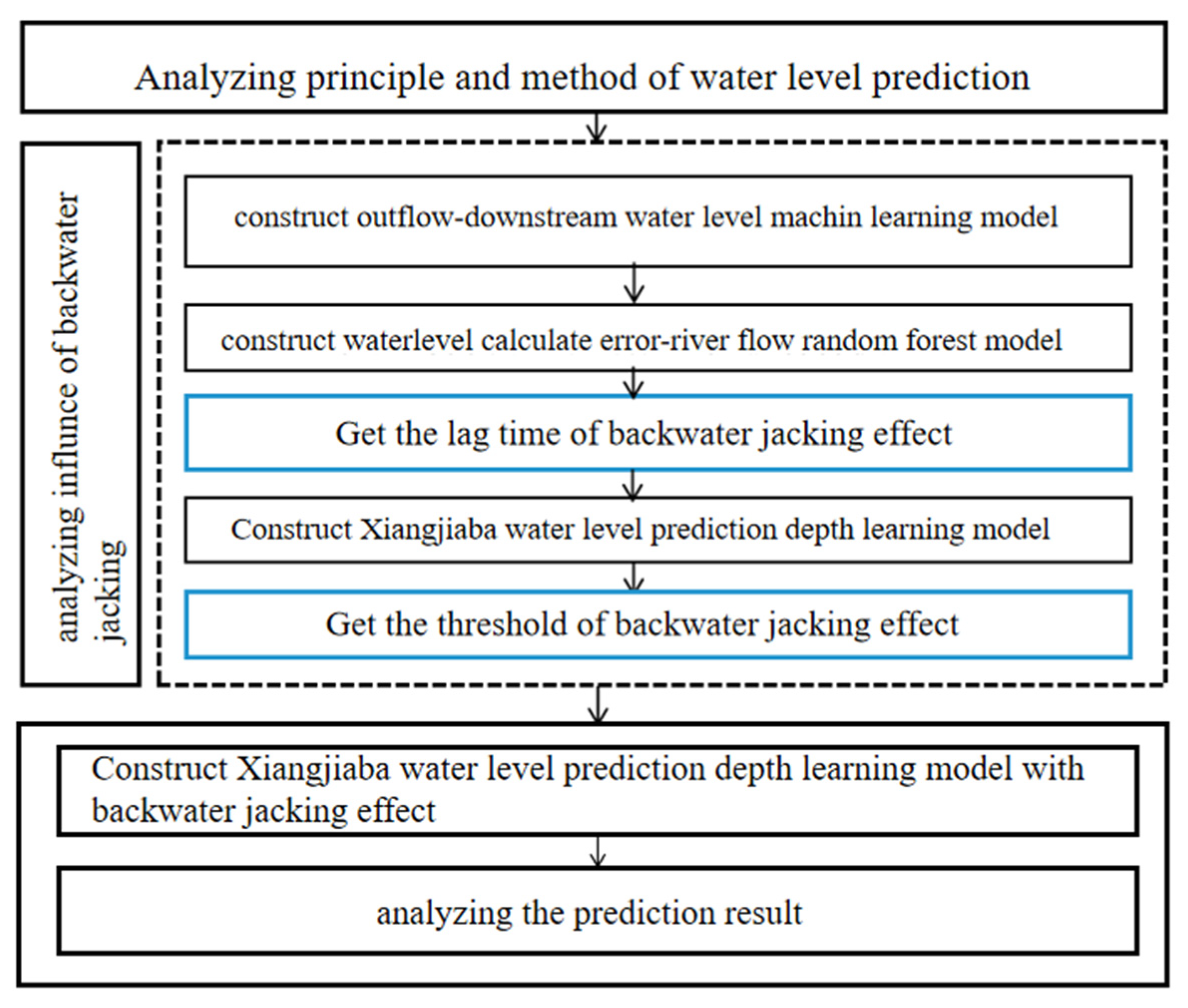
3.1. Analysis Method of Backwater Effect
The analysis of time lag can be mainly divided into two primary steps. Initially, the linear regression model is employed to establish the corresponding relationship between the TWL of the XJB and the outbound flow rate; in this way, the prediction error between the calculated TWL of the XJB and the actual TWL is determined. Additionally, a relationship between the prediction error of the TWL and the run offs of the Hengjiang River (HJR) and the Minjiang River (MJR) before different hours is established. By utilizing the run offs data with different time lags as input variables and the water level prediction error as the output variable, the random forest model can be employed to calculate the significance of various input factors. This analysis aids in identifying the specific time lag from which the error predominantly originates, focusing on the run offs data of the correct time.
The threshold analysis builds upon the outcomes of the lag analysis. A 12 h prediction model without considering the backwater effect is established. This model allows for the categorization of different scenarios based on the varying run offs of the HJR and the MJR. By computing the water level prediction error under different scenarios, it becomes evident that scenarios with run offs exceeding the backwater effect threshold exhibit notably higher prediction errors compared to those under the threshold.
3.2. Time Lag Analysis of Backwater Effect
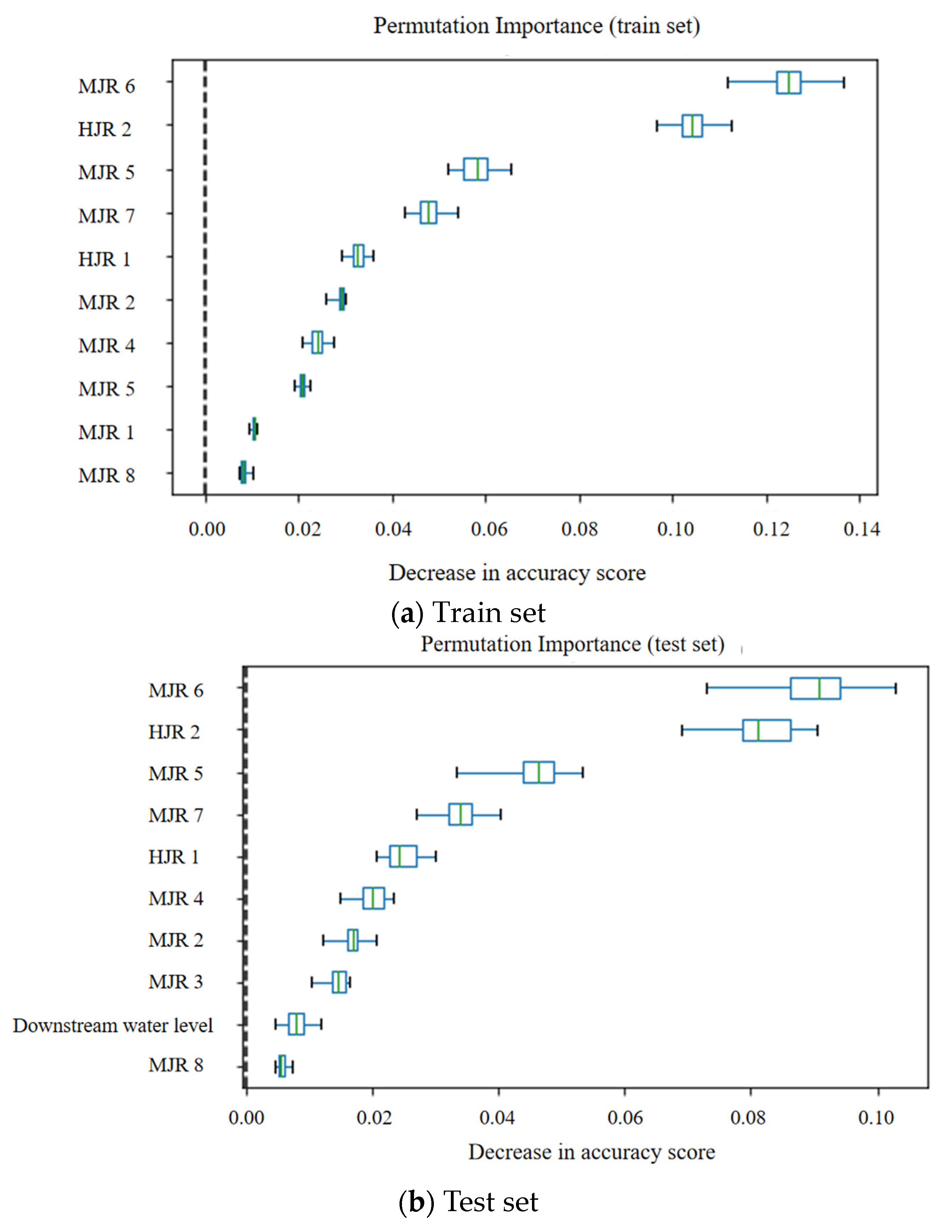
The random forest model employs a technique wherein the ordering of feature factors within the training set is randomly shuffled to analyze their individual impact on the resultant output variable. In the context of this study, a random forest model was constructed with the run offs of the HJR and the MJR at different time lags serving as input factors, while the TWL of the XJB error, calculated through machine learning methods, was set as the output. The model aimed to determine the characteristic weights between the run offs of the HJR and the MJR at various time lags on the water level error. In the analysis process, the calculation was repeated 30 times, and the influence degree of different time periods of the HJR’s and the MJR’s run offs on the prediction error was drawn as a box diagram, as in
Figure 6. The
y-axis in the figure represents different input factors. The ‘MJR 6’ represents the flow rate of the MJR six hours ago. Other input factors follow a similar pattern. On the
x-axis, the decline in the model index resulting from the random disruption of each factor is depicted, thereby capturing the importance of the perturbed factor to the output variable.
The presented figure demonstrates that both the test set and the training set exhibit identical distributions in terms of the calculation of characteristic importance. The top five factors of the two sets are the same, which are Minjiang river 6, Hengjiang river 2, Minjiang river 5, Minjiang river 7, and Hengjiang river 1. The results show that the lag time of the backwater effect of the MJR run off to the TWL of the XJB is about 5–7 h, and that of the HJR run off to the TWL of the XJB is approximately 1–2 h.
3.3. Threshold Analysis of Backwater Effect
The backwater effect threshold analysis method utilizes a deep learning model to predict the tail water level (TWL) of the XJB under different scenarios, and the model disregards the influence of the backwater effect. This analysis involves the segmentation of flow scenarios from the Hengjiang River (HJR) and the Minjiang River (MJR). Specifically, the analysis focuses on prediction and computation using data from the year 2019, and the scenarios are categorized based on predefined thresholds (700 m
3/s for HJR run off and 7000 m
3/s for MJR run off). These thresholds divide the scenarios into two types: Scenario 1, where either the HJR flow rate or the MJR flow rate exceeds their respective thresholds, and Scenario 2, where both flow rates are below their thresholds. Additionally, an overall scenario without threshold division is also considered. The 12 h prediction errors for three scenarios are visualized in
Figure 7.
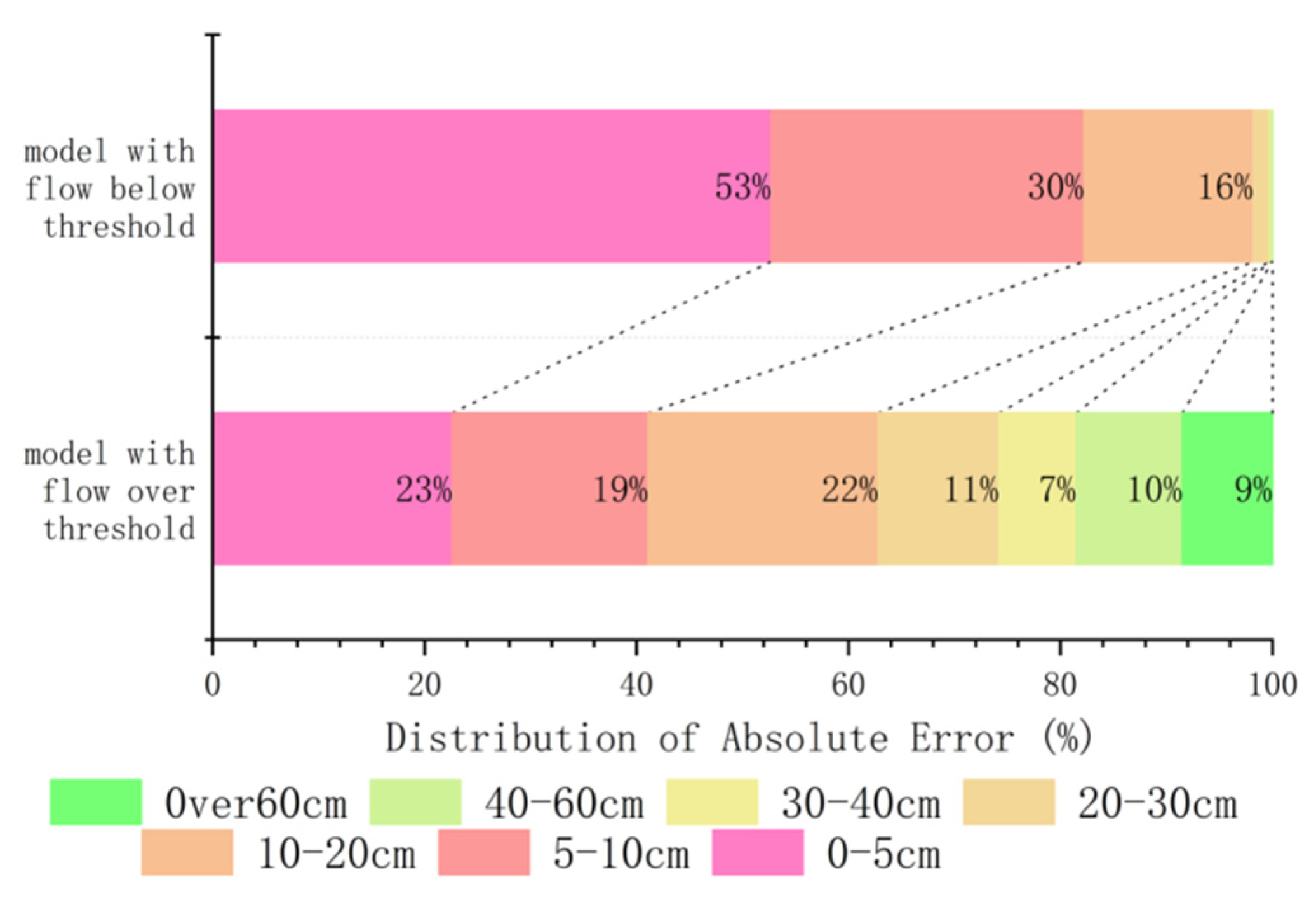
The maximum prediction error of the overall scenario coincides with that of Scenario 1, while the average prediction error of Scenario 1 is much higher than that of the overall scenario and Scenario 2. The error distribution diagram of different scenarios is shown in
Figure 8.
From the distribution of errors, in Scenario 1, 18.49% of the errors are above 40 cm, while in Scenario 2, only 0.04% of the errors exceed 40 cm. Overall, using 700 m3/s as the threshold for the HJR flow rate and 7000 m3/s as the threshold for the MJR flow rate can effectively differentiate between forecast scenarios. When both flow rates are below the threshold, the maximum absolute prediction error is 55.02 cm, and the average prediction error is 5.93 cm. In comparison, it can be assumed that this scenario is minimally impacted by the backwater effect.
4. Analysis of Predictive Performance
4.1. Prediction Result of the WBE Model
Using the method described earlier, a Water Balance Error (WBE) model was formulated to assess the TWL of the XJB in 2020, employing a time step interval of two hours. The resultant absolute error measurements are presented in
Figure 9, providing an informative illustration of the model’s performance.
The evaluation of the results demonstrates a mean absolute error of 47.3 cm, with a maximum absolute error of 878.3 cm. Errors exceeding the 100 cm threshold constitute around 10% of the total errors. During the calculation process, it was observed that the error in the discharge flow exiting the XJB is less than 3%, indicating high accuracy. Consequently, the primary source of discrepancy in the estimation of the tail water level (TWL) of the XJB can be ascribed to two factors: the imprecision inherent in the TWL empirical curve and the backwater effect generated by the HJR and the MJR beneath the XJB dam.
4.2. Prediction Result of LSTM Model
The model of the backwater effect threshold analysis does not incorporate the influence of rainfall within the stream direction interval, and it solely relies on the inflow of the XJB as the input parameter, which hampers its practical applicability. To address this limitation, a revised prediction model is proposed, wherein the inflow of the XJB is substituted with XLD output, XLD abandoned water, and rainfall within the stream direction interval. By adding these variables, the prediction model is rendered more suitable for practical applications. Notable characteristic variables considered in the model encompass the variables presented in
Table 2.
In the analysis, it is recognized that the forecast data used in the model contain inherent errors, and the impact of these errors on water level prediction remains unclear. Additionally, the backwater effect of the HJR and the MJR, as well as the conversion of rainfall into run off and inflow, entail a time lag. Consequently, when the forecast period is short, utilizing historical flow rate and rainfall data from the HJR, MJR, and XJB can enhance the predictive capabilities of the model and enhance its practicality. To compare the predictive performance of different forecast periods, three prediction models for the XJB’s TWL are constructed: a 12 h forecast, a 24 h forecast, and a 48 h forecast, each with a step of 1 h. The error statistics of different forecast periods are shown in
Figure 10.
The error distribution of each model across different forecast periods shows a similar pattern, without any significant exceptions. Upon comparing the models, it is observed that the 12 h forecast model yields the most accurate predictions overall. It exhibits a mean absolute error of 3.43 cm and a maximum absolute error of 30.74 cm. These values are lower than the corresponding errors obtained from the previous 12 h of the 24 h forecast model, where the mean absolute error was 3.56 cm and the maximum absolute error was 32.47 cm. Similarly, the 24 h forecast model demonstrates a mean absolute error of 3.93 cm and a maximum absolute error of 45.07 cm, which are lower than the corresponding errors obtained from the previous 24 h of the 48 h forecast model, where the mean absolute error was 6.03 cm and the maximum absolute error was 67.14 cm. Therefore, in the final prediction, a comprehensive approach is taken by combining forecasts from three different models. Specifically, the first 12 h forecast is generated using the 12 h prediction model, the 13 to 24 h forecast is obtained from the 24 h prediction model, and the 25 to 48 h forecast is derived from the 48 h prediction model.
Based on the prediction models of different forecast periods, the overall error distribution within the 48 h forecast period is shown in
Figure 11.
From the graph, specifically, the error in the last 24 h of the forecast shows a noticeable increase compared to the first 24 h. The average absolute error for the initial 24 h is recorded as 3.87 cm, whereas it rises to 6.67 cm for the subsequent 24 h. Similarly, the maximum absolute error also displays an increase, with the value advancing from 45.07 cm in the first 24 h to 63.35 cm in the later period. Overall, when considering the entire range of predictions, the mean absolute error is calculated to be 5.27 cm.
4.3. Result Analysis
Based on the comparison between the WBE (water balance equation) model and the LSTM model and considering the backwater effect, it is evident that the LSTM model performs significantly better in terms of prediction accuracy. The mean absolute error of the LSTM model, which incorporates the backwater effect, is approximately 11%.
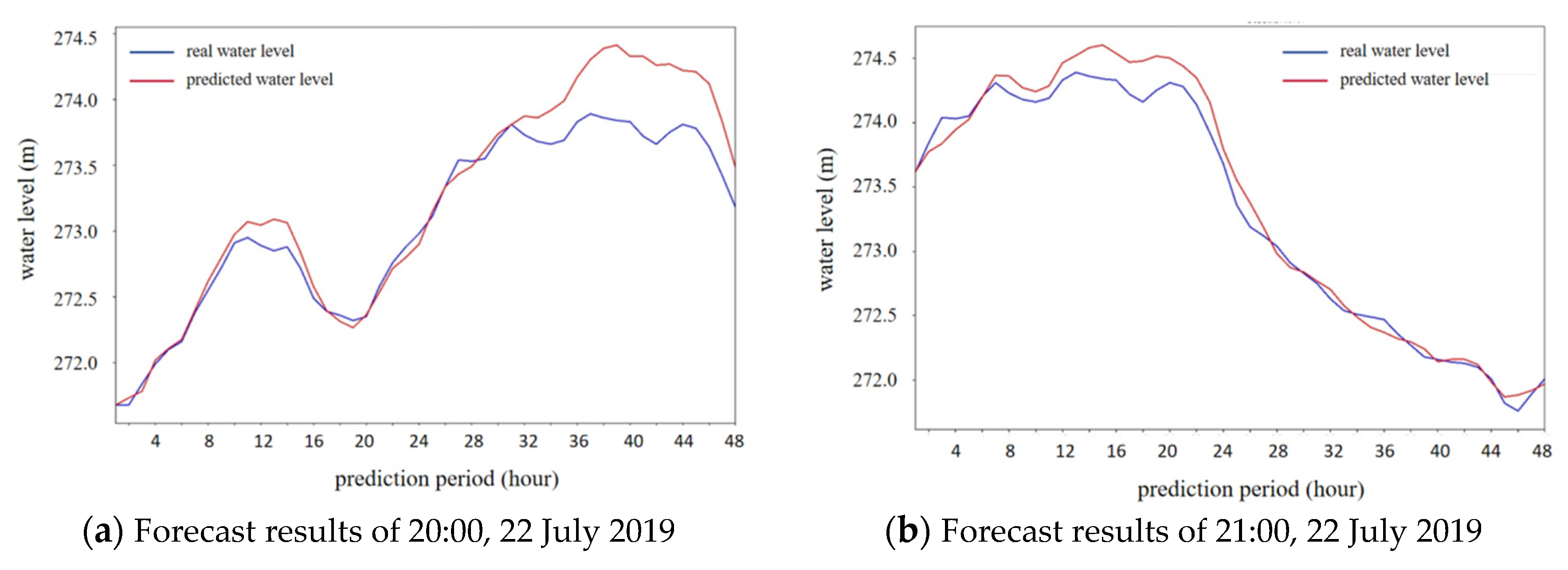
To analyze cases where the error exceeds 60 cm,
Figure 12a illustrates the comparison between the predicted water level process and the measured water level process. When the prediction start time is delayed by one day, meaning that the prediction starts at 21:00 on 22 July 2019, the comparison between the predicted water level process and the measured process is shown in
Figure 12b. It is observed that both the overall error and the maximum water level prediction error decrease. This indicates that utilizing rolling prediction can help mitigate the impact of prediction errors during practical applications.
Figure 13 represents the error distribution of the predicted results between LSTM_Model1, which is the LSTM prediction model without considering the backwater effect constructed in
Section 3, and LSTM_Model2, which is the LSTM prediction model considering the backwater effect constructed in this section. The error distribution plot provides a visual comparison of the differences between the predicted values of the two models. It helps identify the variations in the errors present in their predictions. By analyzing this plot, we can understand the impact of incorporating the backwater effect on the accuracy of water level predictions.
The prediction error of the two models is shown in
Table 3, and the maximum absolute error and mean absolute error have significantly decreased after considering the backwater effect. The mean absolute error was reduced from 7.66 cm to 5.272 cm, and the maximum absolute error was reduced from 217.52 cm to 63.35 cm.
Indeed, deep learning models, such as the LSTM (Long Short-Term Memory) model, often have significant advantages in accurate predictions. The LSTM model excels in handling time series problems, and it can consider many characteristic variables that are challenging to include in traditional calculation-based models, like the WBE (water balance equation) model. Comparing LSTM_Model1 (without considering the backwater effect) and LSTM_Model2 (considering the backwater effect) helps demonstrate the correctness of analyzing the lag time and threshold values associated with the backwater effect.
The substantial reduction in the maximum absolute error indicates that the backwater effect is a significant contributing factor to large errors in predicting tail water levels (TWLs). By incorporating the backwater effect into the models, the stability and reliability of the TWL predictions improve significantly. This highlights the importance of considering the backwater effect when aiming to achieve more accurate and robust predictions using the LSTM model.
5. Conclusions
The application of deep learning and machine learning provides flexibility, powerful computational power, and fitting capabilities in various domains. In addition to using these techniques for prediction based on input feature variables, they can also be employed for feature analysis. This paper aims to develop a deep learning model for predicting tail water level (TWL) considering the backwater effect. To accomplish this, it is necessary to identify the conditions that can lead to the backwater effect in the tributaries downstream of the dam. Subsequently, this information is incorporated as part of the flow variables in the deep learning model for training and prediction. The lag time of the backwater effect is analyzed using the random forest model. The threshold analysis involves dividing different scenarios based on the flow rate of downstream tributaries (the HJR and the MJR) of the XJB. By observing in which scenario the prediction error of the tail water level significantly increases, the threshold value can be determined.
After that, the TWL prediction model based on LSTM considering the backwater effect is constructed. Compared to the WBE model, the accuracy of the prediction results is improved by approximately 90%. Additionally, compared to other deep learning models that do not consider the backwater effect, the accuracy is increased by approximately 30%. The prediction error is controlled within 63 cm. This demonstrates that the application of deep learning methods and neural network models holds great promise in the field of water resources and provides a reliable alternative to traditional calculation approaches.
However, it is important to acknowledge that the model also has limitations. When the number of downstream tributaries of the dam increases, the number of scenarios required for backwater effect threshold analysis will also increase significantly. Each scenario necessitates model training and prediction, leading to a substantial increase in the time required for threshold analysis. Consequently, exploring a new method to determine the backwater effect threshold more quickly is an improvement direction of the model and the next goal of this study.


