Reconstruction of Snow Cover in Kaidu River Basin via Snow Grain Size Gap-Filling Based on Machine Learning

Abstract

Fine spatiotemporal resolution snow monitoring at the watershed scale is crucial for the management of snow water resources. This research proposes a cloud removal algorithm via snow grain size (SGS) gap-filling based on a space–time extra tree, which aims to address the issue of cloud occlusion that limits the coverage and time resolution of long-time series snow products. To fully characterize the geomorphic characteristics and snow duration time of the Kaidu River Basin (KRB), we designed dimensional data that incorporate spatiotemporal information. Combining other geographic and snow phenological information as input for estimating SGS. A spatiotemporal extreme tree model was constructed and trained to simulate the nonlinear mapping relationship between multidimensional inputs and SGS. The estimation results of SGS can characterize the snow cover under clouds. This study found that when the cloud cover is less than 70%, the model’s estimation of SGS meets expectations, and snow cover reconstruction achieves good results. In specific cloud removal cases, compared to traditional spatiotemporal filtering and multi-sensor fusion, the proposed method has better detail characterization ability and exhibits better performance in snow cover reconstruction and cloud removal in complex mountainous environments. Overall, from 2000 to 2020, 66.75% of snow products successfully removed cloud coverage. This resulted in a decrease in the annual average cloud coverage rate from 52.46% to 34.41% when compared with the MOD10A1 snow product. Additionally, there was an increase in snow coverage rate from 21.52% to 33.84%. This improvement in cloud removal greatly enhanced the time resolution of snow cover data without compromising the accuracy of snow identification.

1. Introduction

Snow cover monitoring with fine spatial–temporal resolution has important guiding significance for watershed-scale snow water resource management and sustainable utilization, natural disaster assessment, and early warning in pastoral areas. Spaceborne optical and microwave sensors are important platforms for snow monitoring. However, an optical remote sensing image is sensitive to cloud cover, and it is not possible to obtain information of snow cover under clouds. Exploring the cloud removal algorithm has great significance for restoring the snow condition under the cloud [1].

A large number of studies have shown that snow cover monitoring using optical remote sensing performs with high accuracy. The principle is that snow shows high reflectivity in visible and infrared bands but low reflectivity in the shortwave infrared (SWIR), which is different from other land covers [2]. The normalized difference snow index (NDSI) distinguishes snow pixels by measuring the relative magnitude of the reflectance difference between the visible band (GREEN) and SWIR. The moderate resolution imaging spectroradiometer (MODIS) mounted on Terra and Aqua satellites has provided worldwide stable daily snow cover data for nearly 20 years with its excellent spatial–temporal resolution and good stability [3,4]. However, the similar spectral reflection characteristics of snow and cloud in the visible and near-infrared bands, especially the similar spectral response of cirrus cloud and snow in the whole infrared spectrum, results in the misjudgment of snow and cloud [5]. In addition, there are still a large number of cloud pixels in the daily snow cover data of MODIS, which affects the spatial scope of snow monitoring, the accuracy of snow cover mapping, and the temporal resolution of snow, and limits the further application of optical remote sensing snowpack products. Therefore, many scholars have carried out a lot of research on cloud removal of snow remote sensing to improve the temporal resolution of snow cover [6]. At present, four major methods of cloud removal from snow cover using satellite remote sensing are summarized, the first is temporal filtering-based cloud removal, the second is spatial filtering-based cloud removal, the third is the cloud removal algorithm based on multi-sensor fusion, and the fourth is the cloud removal using snowline elevation.

Gafuov and Bárdossy proposed a cloud removal algorithm from MODIS snow cover products based on temporal filtering [7], which assumes that the snow will not melt quickly in a short time, but the clouds will move quickly. By synthesizing the snow products from Terra and Aqua, the moving clouds are filtered to maximize the snow cover extent. Cloud removal based on temporal filtering can be deduced and calculated without other satellite or ground auxiliary data. For areas lacking multi-source satellite data or relevant geographical parameters, the real snow cover extent can also be calculated.

The aforementioned studies have proved that selecting the appropriate time window and synthetic days to conduct temporal filtering cloud removal can obtain snow cover recognition results with high accuracy, but the step of “Filtering cloud removal during snow accumulation and melting” will cause many false or missed judgments of snow pixels that are fragmented in time series, thus reducing the accuracy of snow cover recognition. Furthermore, the appropriate time window and synthetic days are uncertain and different for different regions and periods. Therefore, large errors will occur when this method is applied to regions with a wide spatial range, strong snow heterogeneity, and long-time series snow data sets. There will be large errors, and the applicability of the algorithm will be greatly reduced. The core of the spatial filtering cloud removal method is to select cloud-free pixels in the spatial neighborhood to estimate the ground coverage under the cloud. In the spatial filtering cloud removal strategy proposed by Gafurov and Bárdossy, there are the “Near four-pixel method”, “Near eight-pixel method”, and other methods. The cloud removal algorithm based on spatial filtering can be deduced and calculated without other satellite data. Simultaneously, in practical application, although the amount of cloud removal of this algorithm is less, it also maintains the lowest error.

The cloud removal method based on temporal filtering and spatial filtering mainly uses the temporal and spatial variation of snow cover of the same optical remote sensor to extract the ground information under the cloud. In contrast, another cloud removal method based on multi-source data fusion uses complementary information between different data sources, such as optical remote sensing observation, microwave remote sensing observation, and station observation [8,9,10]. But the distribution and number of meteorological stations limit the prediction ability of this method for snow reconstruction. However, the above research can only qualitatively infer the distribution of snow cover under clouds, lacking quantitative characterization of snow cover parameters under clouds.

In recent years, researchers have been striving to use spatiotemporal information for one-step cloud removal algorithm research. Xia et al. [11] introduced variational interpolation to construct a three-dimensional implicit function containing five consecutive day data, which can easily obtain the shape of the snow cover boundary. The cloud removal method proposed by Poggio and Gimona [12] is a combination of a generalized additive model (GAM) and a geostatistical spatiotemporal model. The multidimensional spatiotemporal GAM models binary variables, and geostatistical kriging methods are used to explain spatial details. This method utilizes auxiliary data such as surface temperature, land cover, and soil type to effectively simulate the spatiotemporal correlation of snow cover and can achieve satisfactory reconstruction accuracy even under high cloud cover. The adaptive spatiotemporal weighting method [13] estimates the snow cover of cloud pixels by combining adaptive weights based on the probability of snow cover in space and time, which can completely remove the cloud layer. Huang et al. [14] established a hidden Markov random field framework to remove cloud pixels from MODIS binary snow cover data. This method effectively utilizes spatiotemporal information and achieves an overall accuracy of 88.0% for the restored snow cover range under the cloud. Additionally, the conditional probability interpolation method [8] can effectively calculate the conditional probability of snow pixels being covered by clouds and meteorological data to remove clouds, but this method has limited capacity for removing clouds in areas with few in situ observations. Furthermore, Chen [15] proposes a conditional probability interpolation method based on a space–time cube (STCPI), which takes the conditional probability as the weight of the space–time neighborhood pixels to calculate the snow probability of the cloud pixels, and then the snow condition of the cloud pixels can be recovered by the snow probability. However, existing one-step cloud removal algorithms that utilize spatiotemporal information have significant time computational costs and require multiple auxiliary data, which to some extent limits the application of the algorithm. In addition, the progress of machine learning and deep learning technology has also led to new developments in remote sensing snow cover mapping. Luan et al. proposed an m-day dynamic training strategy, which divides a long-term snow cover mapping task into multiple short-term tasks with consecutive m days and reduces the problems caused by changes in snow cover over time. This strategy is applied to random forest models for binary snow cover (BSC) mapping and fractional snow cover (FSC) mapping, achieving higher accuracy than other training strategies [16]. A new algorithm based on a machine learning method was designed to improve FSC retrieval from brightness temperature, considering other auxiliary information, including soil property, land cover, geography information, and the overall accuracy of the above method reached 0.88 [17]. Guo [18] trained the DeepLap v3+ model using a transfer learning strategy to overcome the computational time and resource consumption of deep learning models. The feasibility and effectiveness of automatically extracting snow cover were demonstrated on high-resolution remote sensing images. Hu trained random forest models using combinations of multispectral bands and normalized difference indices and generated sub-meter and meter-level snow maps based on very-high-resolution images [19]. Liu introduced a highly accurate snow map acquired by unmanned aerial vehicles as a reference to machine learning models, which significantly improved the MODIS fractional snow cover mapping accuracy [20]. Yang et al. are committed to designing a cloud snow recognition model based on a lightweight feature map attention network (Lw-fmaNet) to ensure the performance and accuracy of the cloud snow recognition model [21].

We propose a new strategy for reconstructing snow cover under clouds to achieve the following objectives: (a) exploring the correlation between snow particle size and geographic and meteorological information at the watershed scale, and (b) improving the temporal resolution of snow cover at the watershed scale by filling gaps in SGS and achieving snow mapping for the entire watershed. The organization of the entire article is as follows. After introducing the study area and data preprocessing in Section 2, the methodology for cloud removal and snow cover reconstruction is expounded in Section 3. The results of accuracy verification and mapping will be presented in Section 4. Ultimately, a summary of the research will be described in Section 5.

2. Study Area and Data Preprocessing

2.1. Study Area

The Kaidu River originates from the southern slope of the Central Tianshan Mountain in the northwestern region of China (Figure 1c), traverses through the Small Urdus Basin to the Bayanbulak hydrological station, then turns towards the southeast and passes through Husitaixili and the Big Urdus Basin and along a canyon, and finally flows through Yanqi basin into Bosten Lake. The KRB through which it flows is an important sub-basin of the Tarim River Basin and covers an area of approximately 1.9 × 10⁴ km², with an elevation ranging from 1348 to 4709 m above sea level (m a.s.l). The KRB is located in the hinterland of Eurasia and features a typical warm temperate desert climate. The daily precipitation, temperature, and snow depth data were obtained from the Bayanbulak meteorological station at an elevation of 2458.9 m a.s.l. and were provided by the National Meteorological Information Center of the China Meteorological Administration (http://data.cma.cn/en (accessed on 26 August 2023)). The mean monthly precipitation, temperature, and snow depth for the normal period of 2000–2019 for Bayanbulak are presented in Figure 1a. In this period, the mean annual precipitation was 308.84 mm. The precipitation was mainly concentrated in summer (June, July, and August). More than two-thirds of the precipitation occurred in this season. Because the mean monthly T_min was above 0 °C, precipitation was liquid precipitation. However, the sum of the mean monthly precipitation was only 32.1 mm from October to March. Because the mean monthly T_max was below 0 °C, solid precipitation was mainly concentrated in this period. The snow depth of ground observations was measured manually with a wooden ruler at 8 o’clock every day when more than half of the ground in the field of view around the meteorological station was covered by snow. The measurements were made three times, and the distance between the three measurements was more than 10 m. The measured value was accurate to 0.1 cm. The final snow depth at the station was determined as the average of the three measurements, and an average snow depth of less than 1 cm was recorded as 0. Figure 1b shows the Bayanbulak meteorological station time series of daily snow depth from January 2000 to December 2019. The greatest values of snow depth (35 cm) were found in the winter of 2011. A monthly histogram of the mean snow depth from January 2000 to December 2019 is shown in the inset figure. There was snow in every month except July. The mean monthly snow depth increased from 0.06 to 10.62 cm during August to February and decreased from 7.1 to 0.05 cm during March to June [22,23].

2.2. Satellite Remote Sensing Data

SGS is one of the important parameters to describe the microphysical properties of snow [24,25]. SGS indicates the energy balance state of the snow and is a major input parameter for the snowmelt runoff model and climate model [26]. In addition, the variation of SGS helps to discriminate snow melt area, pure ice area, and snow mound, which is important for the retrieval of snow depth and snow density at the watershed scale. Satellite remote sensing data in the visible (0.4~0.7 μm), near-infrared (0.7~1.4 μm), and short-wave infrared (1.4~2.5 μm) have been widely used for SGS estimation [27,28,29,30].

In this study, the SGS was selected as an important parameter to characterize snow, and SGS under a cloud was estimated by a nonlinear relationship between the distribution of SGS and geographic data. Eventually, the snow information reconstruction under the cloud is implemented. The SGS data used in this study were estimated based on the snow grain size and pollution (SGSP) amount algorithm with careful topographic correction in our previous study [26] for the period of 2000 to 2020 with a spatial resolution of 500 m. The SGS data is calculated and exported based on the Google Earth Engine (GEE) platform after deploying the above algorithm. The specific properties are shown in

Table 1. Attributes of SGS.

Properties	Variable Description
Numerical Range	0–1000 μm (0: Snow-free, Others: Snow)
Data Format	GeoTiff
Space Scope	82.33° E~88.12° E; 42.03° N~44.37° N
Spatial Resolution	0.005° (500 m)
Time Range	27 February 2000~7 May 2020
Time Resolution	Daily

.

The SGS data used in this study have two channels, of which channel 1 is the SGS data retrieval by SGSP and channel 2 is the image classification data. Combining these two channels, the details of the channels are shown in

Table 2. Interpretation of SGS data channel.

Channel 1	Channel 2	Image Classification
0	0	Cloud
0	1	Snow-free
1~1000 μm	0	Snow-cover
1	1	None

.

2.3. Geographic Data

Geographic data includes topographic features such as altitude, slope, aspect, and land cover used to characterize the underlying surface of the snowpack. Topography will affect the accumulation and melting rate of snow, which has a significant impact on the redistribution of snow and the variation of SGS. The digital elevation model (DEM) used in this study originates from the 004 version of the Shuttle Radar Topography Mission (SRTM), with a spatial resolution of 90 m. It is drawn based on the Interferometric Radar of the United States Geological Survey (USGS) and can be downloaded from http://srtm.csi.cgiar.org/index.asp (accessed on 26 August 2023). In addition, topographic features such as slope and aspect are calculated from DEM through ArcGIS.

The difference in land cover will also change the size of the snow grain [31]. MODIS land cover (MCD12Q1) version 6 products are updated year by year for global land cover type. The product has a spatial resolution of 500 m and a period from 2001 to the present. According to the MCD12Q1 reclassification strategy for Western China [32], the land cover in the KRB is reclassified into five types: water, forest, grassland, farmland, and bare land. As shown in Figure 2c, the major land covers in the KRB are grassland and bare land, of which grassland accounts for 84.63% and the area of bare land accounts for 15.36%.

2.4. Ground Observation

The daily snow depth data from 2000 to 2020 observed at Bayanbulak station (Figure 1) of the China Meteorological Administration was used as the “ground truth” values for assessing the accuracy of the gridded snow cover reconstruction data [33,34]. The in situ snow depth measurements are the most accurate record of snow cover, when the snow depth is greater than or equal to 1 cm, the site is snowy, and vice versa, the site is snow-free. Thus, they are widely used for evaluating not only satellite-based snow depth products [32] but also snow cover products [35].

3. Methodology

3.1. Construction of Space–Time Extra Trees Model

Among the current mainstream machine learning algorithms, the random forest (RF) has outstanding performance in both regression and classification. A RF can effectively handle thousands of input samples with high-dimensional features without dimensionality reduction. It is also able to evaluate the importance of each input feature on the objective function. In the algorithm execution, an unbiased estimate of the internally generated error is obtained and a high tolerance for certain missing data is obtained. However, extra trees (ETs) make full use of all samples compared to the Bagging strategy applied with the RF, only the features are randomly selected due to the random splitting, leading to a better regression result than the RF [36]. Also, a RF is used to get the best splitting attributes within a random subset, but ET is used to get the splitting values completely randomly in the global data.

An ET is an integrated machine-learning method developed from an RF [37]. The algorithm is denoted by $\left\{T(V,X,D)\right\}$, where $T$ is the final classifier model, $D$ is the sample set, and $V$ is the number of base classifiers. Each classifier produces a prediction based on the input samples. The execution steps of the ET are shown below [38]:

Step 1: Sample selection: Given the original data sample set $D$, the number of samples $S$, and the number of features $W$. In the ET classification model, each base classifier is trained using the full set of samples.

Step 2: Feature selection: The Base classifier is generated from the Classification and Regression Tree (CART) decision tree. At each node splitting, m features are randomly selected from W features, the optimal attribute is selected for each node for node splitting, and the splitting process is not pruned. Step 2 is performed iteratively on the subset of data generated by splitting until a decision tree is generated.

Step 3: Construction of additional trees: Create additional trees and repeat Steps 1 and 2 for V times to generate V decision trees and ET.

Step 4: Regression of result: Test results are generated from test samples based on designed ET, and the prediction results of all basic classifiers are counted. The final result is determined according to the average value of all decision tree outputs.

ET is the random bifurcation of rows and columns of data, which will lead to the generalization ability of ET being stronger than that of RF. At the same time, each regression tree in the ET makes full use of all the training samples and randomly selects the bifurcation attributes on the node bifurcation, which enhances the randomness of the node splitting of the base classifier.

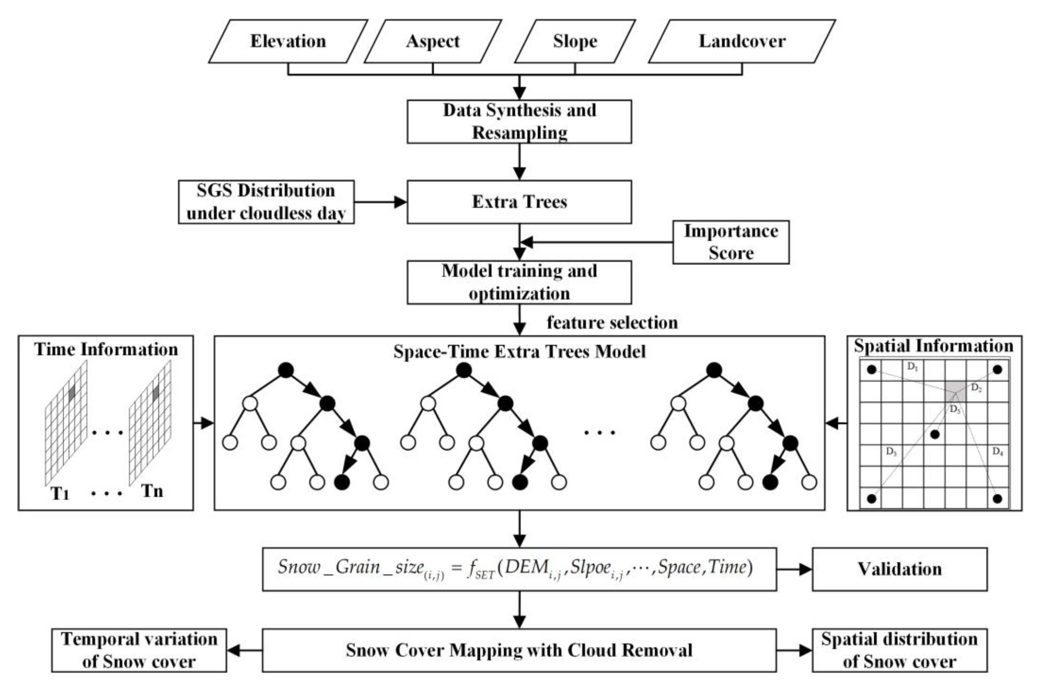
In this study, an SGS filling model based on ET is constructed to implement the reconstruction of snow cover under clouds at the watershed scale, as shown in Figure 3. Geographic elements such as altitude, slope, aspect, and land cover are resampled to 500 m resolution using nearest-neighbor sampling technology as input, and the SGS under a clear sky is used as a sample label. The nonlinear mapping relationship between multi-source data is constructed based on ET.

In the process of model training, importance scores given by the ET can help select the input factors with high importance, optimize the feature selection process of the model, reduce the amount of parameter calculation, and overcome the overfitting caused by parameter redundancy. Simultaneously, considering the spatial distribution information characterizing the SGS and the variation with time, the input data of two-dimensional characterized temporal information and two-dimensional characterized spatial information are designed when training the ET model, and the data about the spatial and temporal information are elaborated as shown in Section 3.2.

3.2. Design of Temporal and Spatial Dimensional Information

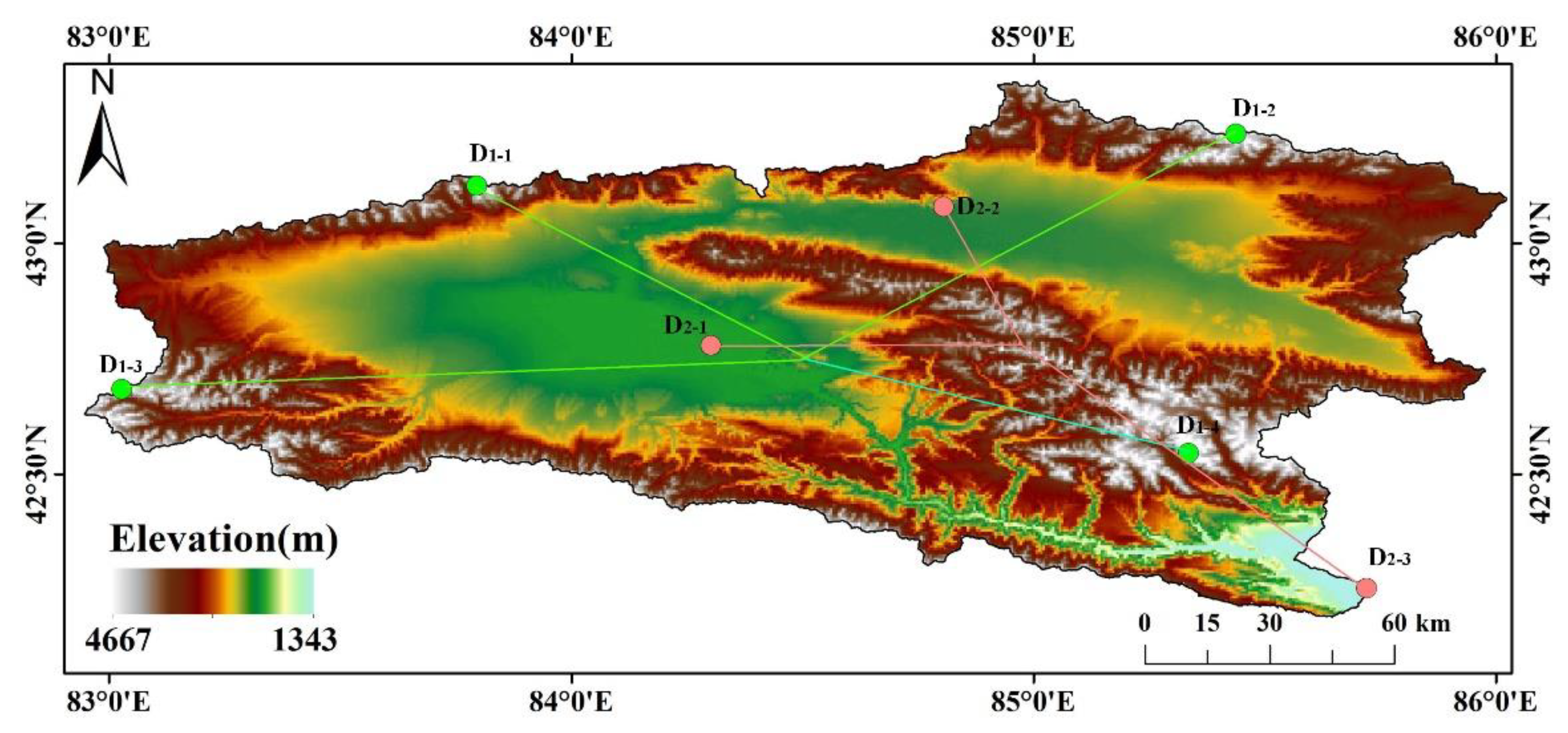
In many previous studies, especially for parameter retrieval at large spatial scales, latitude and longitude were introduced into the model as spatial information parameters to characterize the position of a grid in the whole region. However, it is difficult to accurately quantify the spatial information using latitude and longitude because of the proximity and fine resolution of the grids in the watershed-scale parameter retrieval. In this study, the KRB features a topographic landscape with mountains surrounding the basin, and the Elpin Mountains divide the basin into the Big Urdus Basin and Small Urdus Basins on the east and west sides, forming a typical geomorphic feature of mountains surrounding and blocking the basin. Wei et al. calculated the Haversine distance from each rater point to the upper left corner of the rectangular study area as $D_1$, and analogously, the distance to the upper right corner as $D_2$, the distance to the lower left corner as $D_3$, the distance to the lower right corner as $D_4$, and the distance to the center of the matrix noted as $D_5$, to improve the representation of the model for spatial information [39]. However, the Haversine distance is more suitable for the expression of large-scale spatial information. The study area of the KRB is characterized by high elevation around and low elevation in the middle. We divided the KRB into four quadrants and selected the highest elevation positions of the mountains in four directions in the basin, which are located at (83.7943° E, 43.12466° N), (85.43821° E, 43.23695° N), (83.02624° E, 42.68449° N), and (85.33491° E, 42.54525° N). The Euclidean distance from each grid to the four highest elevation positions was calculated and denoted as $D_{1-1}$, $D_{1-2}$, $D_{1-3}$, and $D_{1-4}$, respectively. $D_1=D_{1-1}+D_{1-2}+D_{1-3}+D_{1-4}$ characterizes the weighted sum of each grid to the highest elevation position in the watershed, as shown by the green line in Figure 4.

Following a similar idea, the lowest elevation positions in Big Urdus Basin, Small Urdus Basin, and Yanqi Basin, located at (84.30185° E, 42.77881° N), (84.80490° E, 43.07975° N), and (85.72118° E, 42.2533° N), respectively, were selected, and the Euclidean distances from each grid to the lowest positions were calculated and denoted as $D_{2-1}$, $D_{2-2}$, and $D_{2-3}$. $D_2=D_{2-1}+D_{2-2}+D_{2-3}$ characterizes the weighted sum of each grid to the lowest elevation position in the watershed, as shown by the pink line in Figure 4. The aforementioned two data $D_1$ and $D_2$ are constructed to improve the model’s representation of spatial information.

Theoretically, the hydrological year is based on the Earth’s hydrological cycle, which begins at the point of return of runoff, which is usually the beginning of the flood season and the end of the dry season. There is some variability in the start and end times in different regions and between years. In the research of snowpack phenology, the hydrological year can also be defined by using the day of onset of snowpack accumulation and the day of final melt as a boundary [40]. In this study, a hydrological year from 1 Sept to 31 Aug of the following year was delineated, taking into account the snowpack characteristics and the characteristics of the study area. The hydrological year is divided into four seasons: spring (March to May), summer (June to August), autumn (September to November), and winter (December to February). The snow cover days (SCDs) of the hydrological year in which the single-view data are located are used as one-dimensional, temporal information, and the SCDs characterize the number of days a grid is covered by snow in a hydrological year. Areas with high SCDs generally have lower temperatures, more snowfall, and more abrupt variability in SGS.

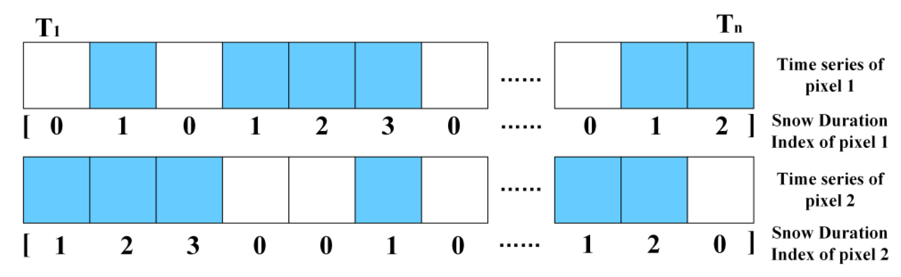
The principle of the second-dimensional temporal information construction is as follows: the grain size of new snow is tiny when in contact with the ground, and the distribution of its grain size shows obvious distribution characteristics that change with altitude and slope. Therefore, the second-dimensional data characterizes the number of consecutive days with snow cover (Snow Duration Index, SDI) at the current moment of a grid, with daily resolution. Compared with the SCDs, the SDI can better reflect the snow status at the current moment. As shown in Figure 5, it represents the state presented by a grid on the time series, where white indicates a snow-free grid and blue indicates a snow grid. Based on the duration of the presence of snow on the time series, the SDI constructed from the 1st grid is $[0,1,0,1,2,3,0,\dots ,0,1,2]$, the SDI constructed from the 2nd grid is $[1,2,3,0,0,1,0,\dots ,1,2,0]$, the 1, 2, 3, and 4 in arrays indicate that the snow has existed for 1, 2, 3, and 4 days, respectively, at the current moment.

3.3. Applicability Evaluation and Factor Optimization of the Model

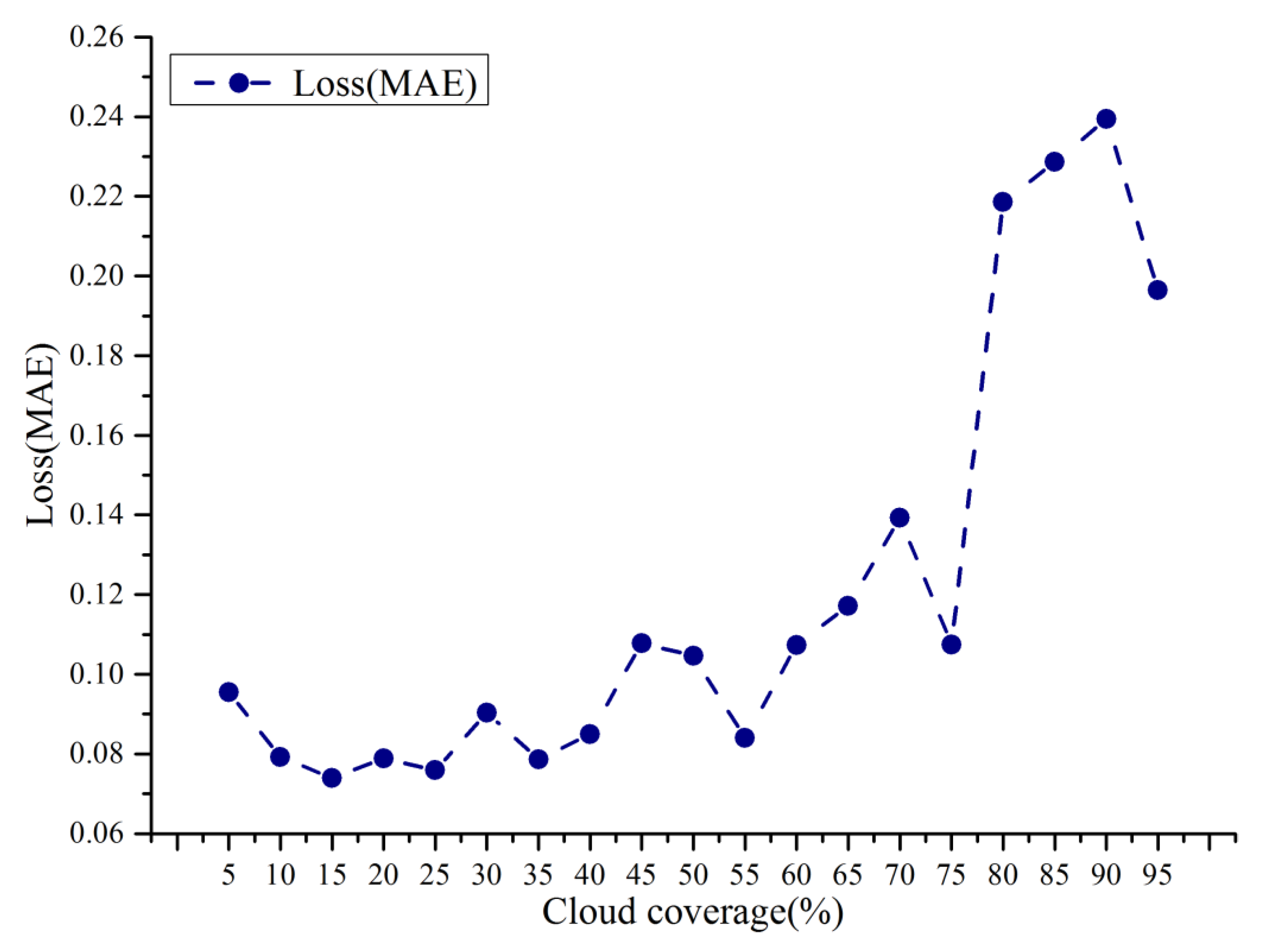
Daily SGS data of the KRB were generated in batches based on the asymptotic radiative transfer model in the GEE for a long series. However, for the SGS data with too much cloud, the mapping relationship between geographic, spatial–temporal information, and SGS cannot be fitted better due to the limited effective training data. Therefore, the training set and test set are divided according to the ratio of 8:2, and the experiments are conducted with different data missing rates (i.e., cloud percentage in the watershed). It can be seen that in Figure 6 the test error increases abruptly when the cloud percentage is greater than 75%. The data missing rate increases to a certain threshold, resulting in too few effective training samples and causing underfitting in model training. Thus, SGS data with cloud coverage below 70% are selected for snow reconstruction in this study.

Under the premise of determining the missing data rate applied to the model, the corresponding altitude, slope, aspect, land cover, spatial dimension data $D_1$ and $D_2$, and temporal dimension data of SCDs and SDI are extracted according to the latitude and longitude, and are used to construct an SGS filling model. The points with an SGS of zero, (i.e., no snow) are also added to balance the snow cover and snow-free surfaces in the model.

In the model training phase, the importance scores are used to evaluate the contributions of the input factors to the results and to optimize the input factors. Since the model is trained for daily images and fills in the missing SGS information to achieve snow reconstruction, the difference in snow status and cloud percentage due to the environmental changes will make the importance scores of input factors ranked differently on each day. In this study, the ranking of the mean importance scores obtained from model training for consecutive years was calculated, as shown in Figure 7. It can be seen that altitude, as the most significant topographic element, is the most important factor influencing the retrieval results, with a score of 0.192. The importance scores of the SDI and SCDs are 0.14126 and 0.13605, respectively, indicating that the present time of the grid at the current moment and the distribution of snow accumulation throughout the hydrological year show a great role in the filling of SGS. While the importance scores of aspects, $D_1$ and land cover were all closer. The lowest importance score is the slope, which is only 0.077, one order of magnitude behind other input factors. Therefore, the importance scores of the hydrological year scale are combined, and altitude, SDI, SCD, $D_2$, aspect, $D_1$, and land cover are finally selected as the inputs of the model for retrieval of SGS under the cloud layer, to realize snow reconstruction. Altitude, aspect, and land cover are geographic information inputs that come into direct contact with snow cover, thereby affecting the SGS through surface temperature conduction, gravity accumulation caused by terrain, and the amount of solar radiation received from different aspects. $D_1$ and $D_2$ further characterize the spatiotemporal properties of snow particles within the watershed, which helps to improve the accuracy of SGS estimation at the watershed scale. SDI and SCD characterize the phenology of snow cover on short and annual time scales, respectively, especially SDI, which is closely related to the evolution and size of the snow grain.

3.4. Snow Recognition of Landsat

Based on the property that both clouds and snow show high reflectance in the visible band, and the difference between the high reflectance of clouds and the high absorption of snow in the short-wave infrared band, the SNOWMAP algorithm [41] was used to identify the snow cover in the Landsat images. In this study, the Normalized Difference Snow Index (NDSI) is calculated in the GEE platform for the green band (band 3) and the short infrared band (band 6) of Landsat-OLI images that have completed radiometric calibration and atmospheric correction, and the threshold of the NDSI for snow identification is set greater or equal to 0.4. The calculation method of the NDSI is shown in Equation (1):

$$\mathrm{NDSI}=\frac{\mathrm{band} 3-\mathrm{band} 6}{\mathrm{band} 3+\mathrm{band} 6}$$

(1)

Given the low reflectance of the water body in both visible and short-wave infrared bands, the threshold of band 5 is set as greater than 0.11 as a way to eliminate the interference of the water body. The combined criterion of $\mathrm{NDSI}\ge 0.4$ and $\mathrm{band} 5>0.11$ can achieve snow identification at 30 m resolution. In the snow binary map, 1 denotes a snow element and 0 denotes a snow-free element.

3.5. Metrics for Evaluating the Accuracy of Snow after Cloud Removal

The accuracy evaluation of snow reconstruction is divided into two parts. The first is the accuracy evaluation of the SGS estimated based on the machine learning model, and the second is the accuracy evaluation of the snow reconstruction results. The root mean squared error (RMSE) and mean absolute error (MAE) between the predicted SGS and the measured SGS are evaluated employing ten-fold cross-validation, and the above indexes are calculated as shown in Equations (2) and (3):

$$\mathrm{RMSE}=\sqrt{\frac{1}{m}{\displaystyle \sum _{i=1}^m{(y_i-{\stackrel{\wedge }{y}}_i)}^2}}$$

(2)

$$\mathrm{MAE}=\frac{1}{m}{\displaystyle \sum _{i=1}^m\left|y_i-{\stackrel{\wedge }{y}}_i\right|}$$

(3)

In the accuracy evaluation system of snow reconstruction, the measured snow depth at the meteorological station is taken as the ground truth, and the ground is judged to be snowy when the snow depth is greater than 1 cm, and vice versa. Based on the aforementioned criteria, the results of snow reconstruction have the following four cases: True Positive (TP), True Negative (TN), False Positive (FP), and False Negative (FN), and the detailed definitions of TP, TN, FP, and FN are described in

Table 3. Four categories of snow reconstruction compared to ground-based observations.

	Ground True	Snow	Snow-Free
Snow Reconstruction
Snow		TP	FP
Snow-free		FN	TN

. TP refers to both snow reconstruction data and ground observation being judged as snow, and TN refers to both being snow-free. FP means that the snow reconstruction data shows snow, while ground observation is snow-free, which generally occurs when the reconstruction misidentifies cirrus clouds as snow, and FN means that the ground observation shows snow, while the snow reconstruction is snow-free, which belongs to snow omission.

Based on the four categories of snow reconstruction data compared with ground observations, a series of performance metrics were introduced to evaluate the accuracy of snow reconstruction by the algorithm in this study and to compare the accuracy with existing snow cover products from MODIS. Based on the ground-based meteorological station observations in the study area, the values of TP, TN, FP, and FN are counted for the period of hydrological years from 2000 to 2020, and the four perspectives of overall accuracy (OA), precision, recall and the combined performance index of F1-score are used to evaluate the performance of snow reconstruction data. The specific formulas for calculating the above four types of indicators are shown in Equations (4)–(7):

$$\mathrm{Overall} \mathrm{Accuracy}\left(\mathrm{OA}\right)=\frac{\mathrm{TP}+\mathrm{TN}}{\mathrm{TP}+\mathrm{TN}+\mathrm{FP}+\mathrm{FN}}$$

(4)

$$\mathrm{Precision}=\frac{\mathrm{TP}}{\mathrm{TP}+\mathrm{FP}}$$

(5)

$$\mathrm{Recall}=\frac{\mathrm{TP}}{\mathrm{TP}+\mathrm{FN}}$$

(6)

$$\mathrm{F}1-\mathrm{Score}=2\times \frac{\mathrm{Precision}\times \mathrm{Recall}}{\mathrm{Precision}+\mathrm{Recall}}$$

(7)

Using the measured snow depth from ground-based meteorological stations as the ground truth to assess the effect of snow reconstruction will result in the problem of underrepresentation due to the sparse stations, taking the KRB as an example, with 20,507 km², while there is only one meteorological station in the basin, Bayanbulak (51,542), with an elevation of 2458 m. As a result, there is a lack of ground truth to evaluate the effect of snow reconstruction in other areas of the basin, especially in high mountain regions. Therefore, after evaluating the accuracy by ground truth, 30 m resolution snow cover derived from Landsat was also used to assess the 500 m snow reconstruction data. The Kappa coefficient is used to calculate the image agreement between snow cover derived from Landsat and snow reconstruction data derived from MODIS, and the formula is shown in Equations (8)–(10):

$$K=\frac{P_o-P_c}{1-P_c}$$

(8)

$$P_o=s/n$$

(9)

$$P_c=(a_1\times b_1+a_0\times b_0)/(n\times n)$$

(10)

where $P_o$ is the actual consistency rate and $P_c$ is the theoretical consistency rate. In Equations (8) and (9), the total pixels of the remote sensing image is $n$, the number of snow pixels in the Landsat image representing the real situation of the ground is $a_1$, and the number of snow-free pixels is $a_0$. In the corresponding snow reconstruction data, the number of snow pixels is $b_1$, and the number of snow-free pixels is $b_0$, $s$ represents the same number of the corresponding pixels in the two images.

According to the literature [42], the Kappa test can be used to represent different levels of consistency using five sets of classifications.

Table 4. Comparison of image consistency levels based on Kappa coefficients.

The Value Interval for Kappa	The Consistency Level of the Image
0 < Kappa ≤ 0.20	Very low consistency
0.20 < Kappa ≤ 0.40	General consistency
0.40 < Kappa ≤ 0.60	Medium consistency
0.60 < Kappa ≤ 0.80	High consistency
0.80 < Kappa ≤ l	Almost complete consistency

illustrates the level of consistency of the two images corresponding to Kappa in different intervals.

4. Results

4.1. Mapping of Snow Cover Reconstruction

The error of SGS estimation will also indirectly affect the result of snow cover reconstruction under the cloud. Therefore, some known SGS data were randomly masked in the model training stage, and the size of the masked snow grain data will be estimated and compared with the original truth.

Table 5. Accuracy comparison of SGS filled by different methods.

Methods	RMSE (μm)	MAE (μm)
Classification and Regression Tree, CART	68.048	49.934
K-Nearest Neighbor, KNN	57.108	42.516
Random Forest, RF	55.822	41.692
Ridge Regression, RR	57.054	45.048
Support Vector Regression, SVR	56.710	42.880
Denoising Autoencoder Artificial Neural Network, DAANN	54.186	40.852
Space–Time Extra Randomized Trees	52.751	40.109

lists the RMSE and MAE of SGS based on the space–time ET model and other mainstream machine learning methods. It can be seen that the space–time ET model proposed in this study performs the best result, with the lowest RMSE and MAE of 52.751 μm and 40.109 μm, respectively.

Based on SGS filling, the minimum value of SGS in the image of that day is taken as the threshold for snow discrimination. If the estimation result is greater than the threshold, it is judged as snow, otherwise, it is judged as snow-free. Two environments of “more snow and less bare land” and “less snow and more bare land” are selected to compare the accuracy of snow cover reconstruction. First, the reconstruction of snow under clouds in the KRB on 6 March 2014, is taken as an example. It can be seen from Figure 8c that the cloud accounts for about 45.62% of the KRB, especially in the mountain area, a large number of pixels are blocked by clouds, and the area of snow accounts for about 47.8%. The snow product is directly used for the estimation of snow areas, which will lead to large errors. After filling the SGS, the complete reconstruction of the snow cover under clouds in the watershed scale is realized, as shown in Figure 8d, and the proportion of snow area has reached 81.5%, increasing the proportion by 33.79%. The kappa coefficient is calculated to evaluate the consistency between the reconstructed snow cover and the Landsat snow cover map. The black part in Figure 8a,b is the area that has not been scanned by Landsat and does not participate in the calculation of consistency. The Kappa coefficient between Landsat’s snow cover map and the reconstructed snow cover map is 32.84%, which is generally consistent but compared with the extremely low consistency of 17.79%, it has been improved by 15.05%. In addition, the scores of OA and F1-score after snow reconstruction increased by 16.88% and 14.5%, respectively, compared with those before cloud removal. The specific accuracy data are listed in

Table 6. Accuracy comparison between Case 1, Case 2, and Case 3 before as well as after snow cover reconstruction.

Accuracy (%)	Case 1: 6 March 2014		Case 2: 21 April 2016		Case 3: 2 November 2017
	Before Reconstruction	After Reconstruction	Before Reconstruction	After Reconstruction	Before Reconstruction	After Reconstruction
OA	64.15	81.03	38.26	88.45	77.46	85.23
Precision	65.28	82.86	4.38	35.74	82.48	88.53
Recall	85.79	95.28	34.24	65.16	81.24	86.68
F1-Score	74.14	88.64	7.77	46.16	81.86	87.60
Kappa	17.79	32.84	6.83	86.74	81.46	86.93

. The snow reconstruction on 21 April 2016, is shown in Figure 8f–j as the second case, with 60.73% cloud coverage. The Big Urdus Basin and Elpin Mountains are covered by generous continuous clouds, and the traditional spatiotemporal filtering makes it difficult to achieve snow reconstruction under a cloud with high accuracy. Based on the SGS filling, the spatial distribution of snow in the Elpin Mountains and the southwest of the basin is restored, and the proportion of snow cover has increased from 7.42% to 8.77%, as shown in Figure 8i, which has good consistency with the Landsat 30 m resolution snow map in Figure 8g. The kappa coefficient of snow reconstruction results and Landsat snow map increased from 6.83% before cloud removal to 86.74%, with almost complete consistency, and the OA index and F1-score also increased by 50.19% and 38.39%, respectively. In addition, this study also selected the snow cover of 2 November 2017 as Case 3. The cloud coverage rate in the KRB region is only 13.08%, which effectively achieves the reconstruction of snow cover in the watershed under low cloud conditions. From Figure 8n, it can be seen that the mountains in the eastern part of the KRB have sustained cloud cover. After filling with SGS, it is estimated that the reconstruction of snow cover on the eastern mountain of the watershed has been achieved relatively well. Compared with the snow cover map of Landsat in Figure 8l, it can better match the spatial details. The kappa coefficients of both, increased from 69.48% to 85.54% after reconstruction. This study also added widely recognized snow cover extent (SCE) data [43] for spatial comparison with the reconstructed snow cover, as shown in Figure 8e,j,o. Taking the Landsat snow cover map in Figure 8b,g,l as the true value, it can be seen that the snow cover reconstruction results based on SGS filling have a more detailed representation in complex mountainous terrain compared to Hao’s SCE and can more accurately depict the distribution characteristics of snow cover in mountainous environments.

Based on the above three cases, whether in the environment of “more snow and less bare land” or “less snow and more bare land”, and under different cloud coverage rates, the snow cover reconstruction based on the SGS filling has achieved good performance.

4.2. Accuracy of Snow Reconstruction and Cloud Coverage Variations

Cloud removal based on SGS filling can realize complete snow reconstruction under clouds with cloud coverage of less than 70% and maintain high accuracy. The method greatly improves the cloud removal rate on the hydrological annual scale. Figure 9 illustrates the comparison between the snow cover days of MODIS products and reconstructed snow cover days on the hydrological annual scale from 2000 to 2020. The annual snow cover days of MODIS products are shown in the first and third columns, and the reconstructed snow cover days are in the second and fourth columns. It can be seen from the figure that the mountains around the basin and the Elpin Mountains in the middle are the areas with the most significant increase in snow cover days. As the region with the most abundant snow resources in the basin, the good performance of cloud removal in mountains is helpful to the accurate calculation of snow resources. According to the comprehensive analysis in

Table 7. Comparison of SCD before and after snow reconstruction at the hydrological year scale.

Hydrological Year	Trainable Days	Un-Trainable Days	SCD of MODIS	SCD of Reconstructed Snow	SCD of the Station
2000–2001	216	149	46	104	159
2001–2002	244	121	22	83	111
2002–2003	234	131	3	3	16
2003–2004	252	114	44	72	78
2004–2005	229	136	59	103	144
2005–2006	246	119	58	108	148
2006–2007	243	122	29	40	49
2007–2008	248	118	31	39	29
2008–2009	227	138	58	75	110
2009–2010	225	140	67	90	127
2010–2011	256	109	78	142	173
2011–2012	238	127	69	77	89
2012–2013	236	129	39	74	124
2013–2014	250	115	69	99	137
2014–2015	225	140	63	87	116
2015–2016	215	150	35	94	134
2016–2017	231	134	64	96	141
2017–2018	229	136	54	92	146
2018–2019	228	137	53	94	136
2019–2020	221	144	85	122	146
Mean days	234.65	130.45	51.30	84.7	115.65

, the number of days in the KRB where the daily cloud coverage is less than 70% ranges from 215 to 256 during the period of 2000~2020, and the mean days that can be applied to the SGS filling is 243.65, accounting for 66.75% of the whole year. Bayanbulak (51,542), the only meteorological station in the KRB, has an average annual snow cover of 115.64 days from 2000 to 2020, while the average annual snow cover days calculated based on MODIS Snow products are only 51.3 days, which is only 44.36% of the true observation data. The method in this study only reconstructs the snow cover under a cloud for an average of 66.75% of the data every hydrological year and increases the average annual snow cover days of Bayanbulak based on remote sensing observation to 84.7 days, accounting for 73.24% of the true data. In addition, the difference between the reconstructed SCD after cloud removal and the SCD before cloud removal is shown in Figure 10. The SCD difference on the mountains around the KRB and the southeast side of the watershed is the largest, indicating that snow mapping in complex mountainous environments is prone to interference from cloud cover. However, the method used in this study effectively achieves snow removal and reconstruction in complex mountainous environments.

Based on the analysis of the increase in snow cover days in the whole basin and meteorological stations on the hydrological annual scale, the accuracy of reconstructed snow cover data from 2000 to 2020 is further analyzed based on the station data. As shown in

Table 8. Comparison of performance of snow data before and after snow cover reconstruction.

Snow Cover Data	Annual Average Accuracy (%)				Average Annual Coverage (%)
	OA	Precision	Recall	F1	Snow	Cloud	Snow-Free
MODIS Snow	93.69	82.54	86.67	84.55	21.52	52.46	26.02
Reconstructed snow	92.96	83.91	89.02	86.39	33.84	34.41	31.75

, compared with the MODIS snow products, the reconstructed snow cover data only decreased by 0.73% in the OA index, and the precision, recall, and F1-scores increased by 1.37%, 2.35%, and 1.84%, respectively. Combining 66.75% reconstructed snow cover data and 33.25% unreconstructed snow cover data, the average annual cloud coverage decreased from 52.46% to 34.41%, while the average annual proportion of snow cover and snow-free surface increased to 33.84% and 31.75%, respectively.

This study focuses on the weekly scale to analyze the cloud removal and snow cover reconstruction. As shown in Figure 11, it can be seen that the weekly average cloud coverage ranges from 35% to 65%, reaching the highest around the 30th week (i.e., around March). After the SGS filling, the weekly average cloud coverage decreased by about 20%. During the period of mid-November to mid-March, the average snow cover increased by more than 20%. The rest of the time, the increased proportion of snow cover is limited due to less snowfall in the KRB. In general, the weekly average cloud coverage decreases by 20%, while the removed clouds are mainly filled with snow in winter and spring, and mainly filled with a snow-free surface in spring and autumn, which is also consistent with the temporal distribution of snow in the basin.

4.3. Validation of Individual Snow Cover Mapping

Since there is only one ground observation station in the study area, observations based on one station cannot provide representative evaluations of the advantages and limitations of the proposed method. The original snow cover data with the least cloud cover were used for validation purposes [7]. Several days with the least cloud-covered snow data were filled by clouds of other dense cloud-covered snow data. In this way, we could generate “observed” snow cover products where the performance of the proposed method can be validated.

For validation purposes, 8 October 2015 (validation day 1), 20 April 2016 (validation day 2), 25 April 2018 (validation day 3), and 1 June 2018 (validation day 4) were selected because of the least cloud coverage observed on these days. For validation day 1, the original snow cover data from this day with 0.25% cloud coverage was filled by the cloud cover values of 9 October 2015 snow cover data. The cloud cover fraction of the study area on 9 October 2015 was 54.62%. For validation day 2, the satellite observed less cloud cover with only 1.05% over the KRB. The original cloud cover pixels from 21 April 2016 with 60% cloud fraction were assigned to this day for validation purposes. For validation day 3, the original snow cover data from this day with 3.44% cloud coverage was filled by the cloud cover values of 24 April 2018 snow cover data. The cloud cover fraction of the study area on 24 April 2018 was 45.89%. For validation day 4, the satellite observed less cloud cover with only 0.05% over the KRB. The original cloud cover pixels from 2 June 2018 with 41.58% cloud fraction were assigned to this day for validation purposes. The generated snow cover maps with assigned cloud cover pixels were used as an input for a proposed method and the results were compared with the original snow cover data without cloud filling. The detailed validation results are shown in Figure 12 and

Table 9. Validation of individual snow cover mapping.

Accuracy (%)	Validation Day 1		Validation Day 2		Validation Day 3		Validation Day 4
	Our’s	Hao’s	Our’s	Hao’s	Our’s	Hao’s	Our’s	Hao’s
OA	92.89	94.43	86.99	92.58	91.44	89.45	95.77	94.96
Precision	70.12	75.23	87.55	78.54	80.34	69.02	73.13	63.72
Recall	90.40	87.65	54.69	91.52	90.84	96.62	76.21	65.80
F1-Score	78.98	80.97	67.32	84.53	85.27	80.52	74.64	64.75
Kappa	74.78	77.72	59.74	79.69	79.26	73.56	72.33	62.03

.

As can be seen from the table and figure, the validation results reflect that the proposed cloud removal algorithm achieves or even surpasses Hao’s method. Taking validation day 3 as an example, the proposed method outperforms Hao’s method in all indicators except Recall. More importantly, the detailed features of the snow cover data reconstructed by the proposed method for cloud removal are more significant, demonstrating the changes in the trend of snow cover along mountain ranges. However, traditional spatiotemporal filtering and multi-sensor fusion methods have achieved good results in cloud removal and snow cover reconstruction, but they cannot effectively represent fine snow pixels. The proposed method is based on the spatiotemporal distribution of SGS within the entire watershed system, and then it reconstructs the distribution of snow under the cloud. Therefore, the reconstruction results consider the distribution characteristics of snow within the watershed. However, the methods of spatiotemporal filtering and multi-sensor fusion only focus on cloud pixels and their surrounding pixels, lacking large field observations and trade-offs.

Overall, the proposed method is a new exploratory study of the snow cover reconstruction of cloud removal. Its advantage lies in the accuracy index of snow reconstruction reaching or even surpassing traditional cloud removal schemes. However, its limitation is that it is only applicable when the cloud coverage is less than 70%, as excessive cloud cover can lead to insufficient training samples and affect the cloud removal effect.

5. Discussion

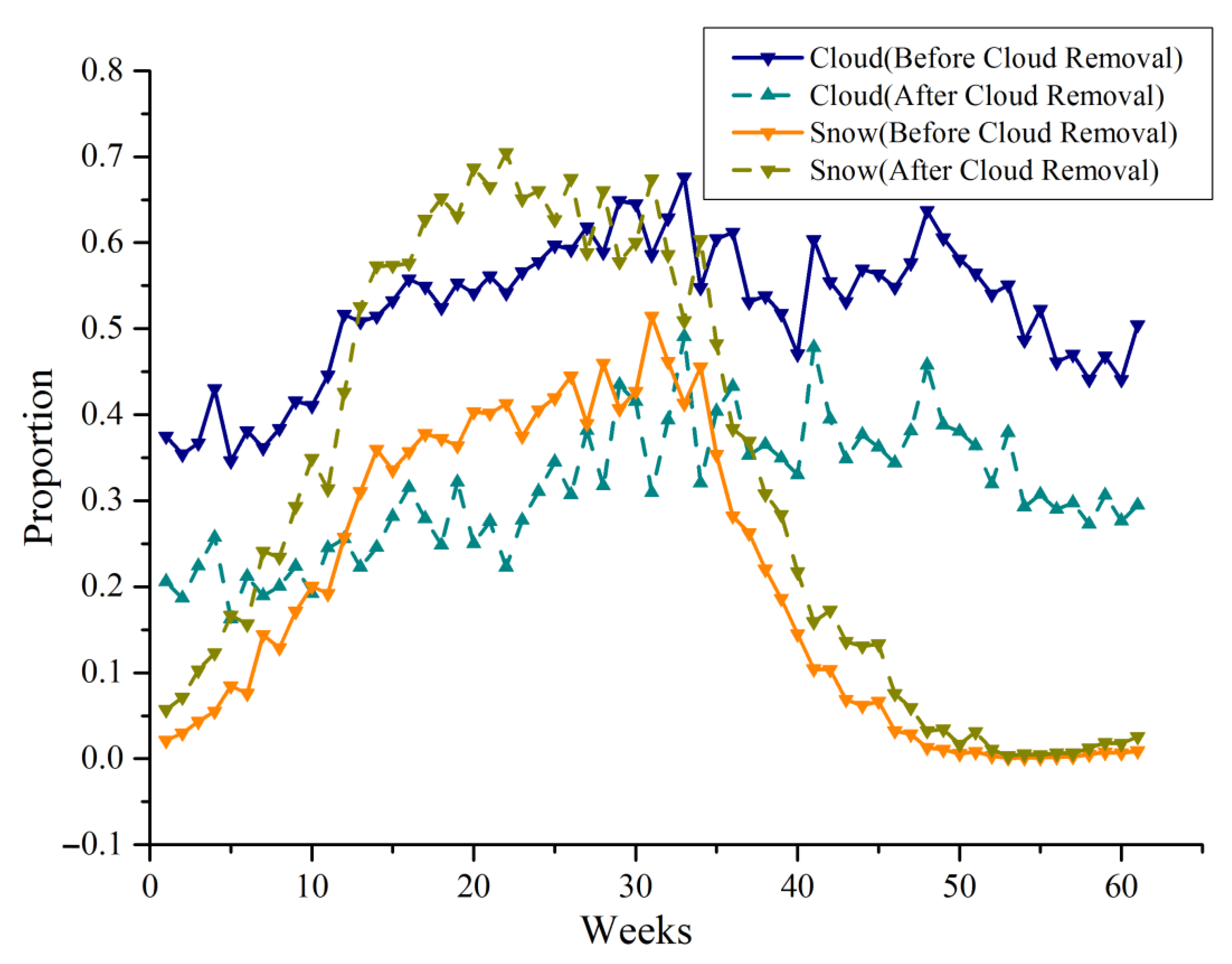
The objective of this study was to remove cloud-covered areas from the original MODIS snow cover products to obtain snow cover information for data-limited regions such as the KRB where no abundant snow cover data is available locally. As stated in Section 4.2, combining 66.75% reconstructed snow cover data and 33.25% unreconstructed snow cover data, the average annual cloud coverage decreased from 52.46% to 34.41%, while the average annual proportion of snow cover and snow-free surface increased to 33.84% and 31.75%, respectively. As a comparison, the spatiotemporal filtering method in a previous study [43] can remove 21.47% of cloud coverage from the KRB, increasing the annual snow cover rate from 20.34% to 41.81%. The SCE data, which has undergone spatiotemporal filtering and cloud removal, has an average annual accuracy of approximately 93% based on site validation in the KRB, slightly higher than the 92% OA of the proposed method. Multi-sensor fusion can further remove 2.59% of cloud coverage and achieve cloud-free mapping of the KRB, with an average annual snow cover rate of 44.40%. Under the condition of complete cloud removal, the overall accuracy based on site verification decreased to 89%, indicating that the uncertainty of multi-sensor cloud removal in complex mountain environments is relatively high. From this point of view, the proposed method in this study maintains higher snow recognition accuracy after cloud removal. The limitation of this study is that it cannot achieve cloud removal of all data on an annual scale.

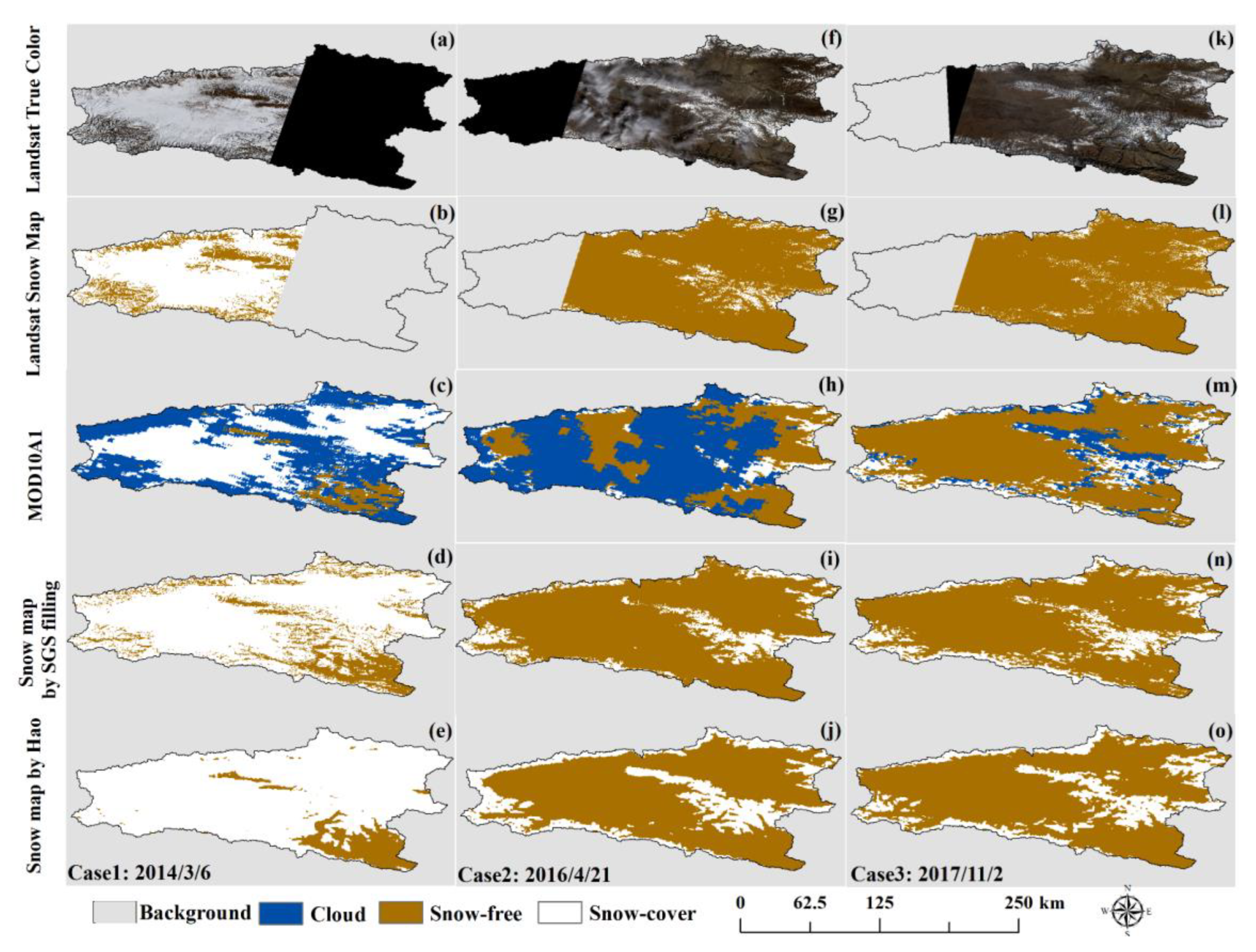
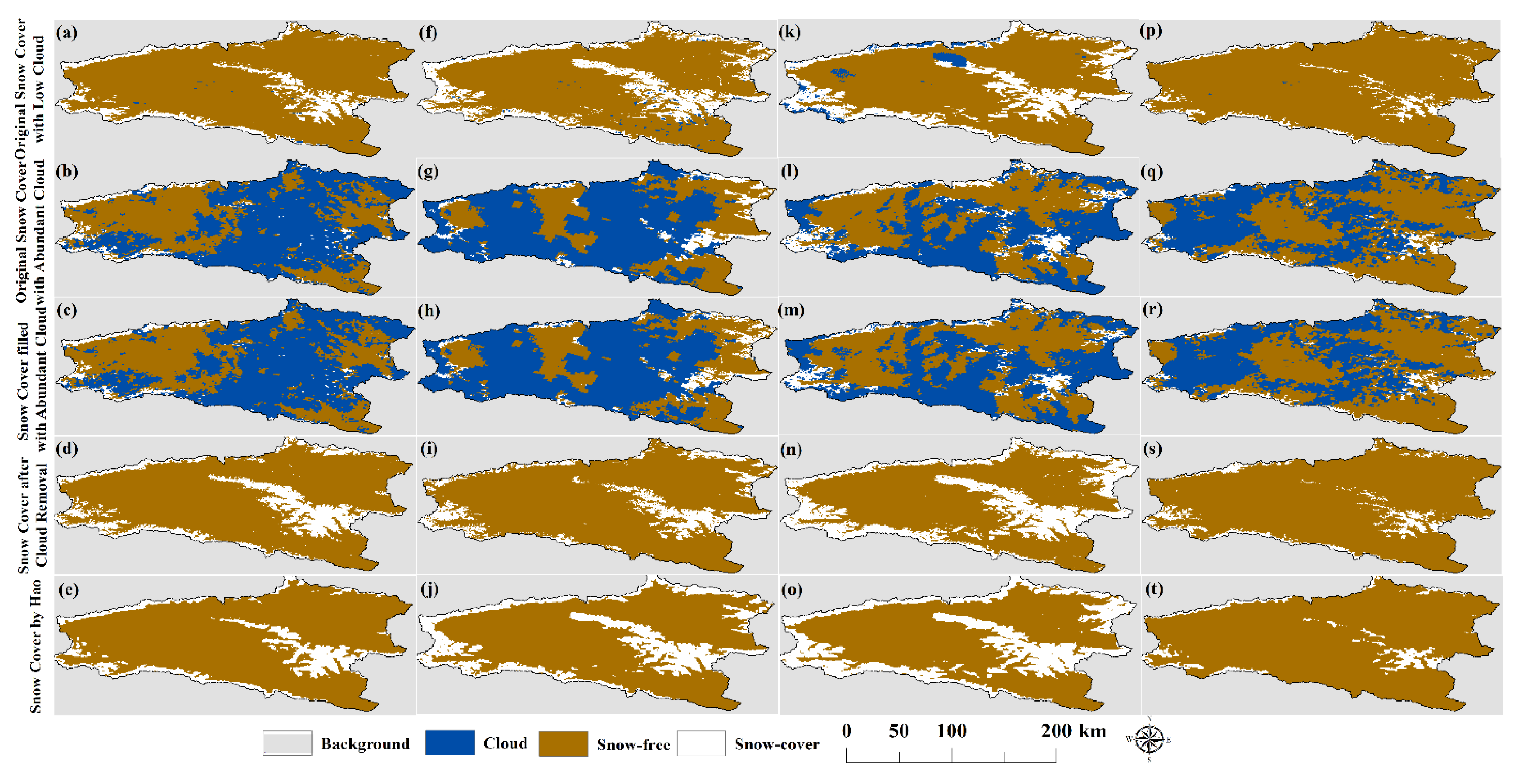
Except for differences in specific accuracy indicators, the proposed method provides more detailed and consistent mountain trends in restoring snow cover under clouds, as shown in the comparison between Figure 12i and Figure 12j. This may be because this method is based on continuous numerical retrieval, which is then used to obtain the value of SGS and determine the snow cover. Moreover, the method in the article mainly relies on cloud pixels themselves or small-scale neighborhood information, lacking overall feature extraction for watershed scale. Based on the above expression, the snow reconstruction-based method on SGS gap filling can be extended to the reconstruction of other missing data (continuous values), such as the reconstruction of ground temperature under clouds and the filling of soil moisture under clouds. For the reconstruction of snow cover under clouds, the proposed method can also be extended to use parameters such as snow density and snow wetness to reconstruct snow cover under clouds [12].

6. Conclusions

The “spatiotemporal” dimensional data that can fully characterize the geomorphic characteristics of the KRB and temporal characteristics of snow was designed and constructed as input data. At the same time, based on the physical characteristics of the variation of SGS with altitude, slope, aspect, and land cover in the watershed scale, the daily SGS filling algorithm of the space–time ET model is constructed and trained, so that the snow cover reconstruction under clouds in the KRB is realized. The algorithm applies to the daily data with a missing rate of less than 70% (i.e., the cloud coverage is less than 70%). A total of 66.75% of snow products have realized the snow cover reconstruction under the cloud based on this method from 2000 to 2020. Compared with MOD10A1 snow cover products, the average annual cloud coverage rate decreased from 52.46% to 34.41%, while the snow coverage rate increased from 21.52% to 33.84%. The data source of this study is SGS data derived from MODIS L1B data. The cloud removal algorithm based on SGS gap-filling can be applied to daily data with cloud coverage less than 70% and achieve one-step cloud removal. Daily data with cloud coverage greater than 70% has poor performance when applying this algorithm. Therefore, this part of the data is not within the scope of this study. In summary, on a year-round scale, the cloud removal algorithm reduced the average annual cloud cover rate of the KRB from 52.46% to 34.41%, and 68.25% of the removed cloud pixels were classified as snow cover, while the remaining 31.75% were classified as snow-free surface.

The main contribution of this study is to carry out SGS filling based on the physical characteristics of SGS distribution at the watershed scale for the first time. Different from the traditional spatiotemporal filtering cloud removal algorithm, the proposed method focuses on considering the spatial and temporal distribution characteristics of snow cover across the entire watershed scale and reconstructed snow cover that fits the geographic and meteorological characteristics of the watershed. Therefore, it better realizes the reconstruction of snow information under continuous large-scale clouds, improves the time resolution of snow, and realizes the deep integration of physical mechanisms and machine learning in the field of snow remote sensing. This article is an exploratory study designed and conducted based on the strong correlation between the spatiotemporal distribution of SGS within a small-scale watershed (KRB) and the terrain and meteorological elements of the watershed. On a larger spatiotemporal scale (such as the entire northern Xinjiang), the strong spatiotemporal heterogeneity of snow grain size can lead to the failure of the method in this study. Meanwhile, the algorithm in this study relies on training with a large amount of effective data. When the cloud coverage rate is higher than 70%, the training effect of the model will deteriorate due to the reduction in data volume, which is also a limitation of this study. In the future, we will attempt to conduct relevant research on a broader basin scale and explore the differences in our research methods across different basin scales to obtain more applicable strategies and methods.