Flux Vector Splitting Method of Weakly Compressible Water Navier-Stokes Equation and Its Application

Abstract

Water is a weakly compressible fluid medium. Due to its low compressibility, it is usually assumed that water is an incompressible fluid. However, if there are high-pressure pulse waves in water, the compressibility of the water medium needs to be considered. Typical engineering applications include water hammer protection and pulse fracturing, both of which involve the problem of discontinuous pulse waves. Traditional calculation and simulation often use first-order or second-order precision finite difference methods, such as the MacCormark method. However, these methods have serious numerical dissipation or numerical dispersion, which hinders the accurate evaluation of the pulse peak pressure. In view of this, starting from the weakly compressible Navier–Stokes (N-S) equation, this paper establishes the control equations in the form of flux, derives the expressions of eigenvalues, eigenvectors, and flux vectors, and gives a new flux vector splitting (FVS) formula by considering the water equation of state. On this basis, the above flux vector formula is solved using the fifth-order weighted essentially non-oscillatory (WENO) method. Finally, the proposed FVS formula is verified by combining the typical engineering examples of water hammer and pulse fracturing. Compared with the traditional methods, it is proved that the FVS formula proposed in this paper is reliable and robust. As far as we know, the original work in this paper extends the flux vector splitting method commonly used in aerodynamics to hydrodynamics, and the developed model equation and method are expected to play a positive role in the simulation field of water hammer protection, pulse fracturing, and underwater explosion.

1. Introduction

Water is a very common fluid medium, widely distributed in the ocean and frequently seen in daily life. Usually, it is believed that water is incompressible and its density is constant. But in some situations [1], water is compressible with a slight or significant change of density. A typical example is the water hammer, and water density may slightly change when the water hammer appears. Another example is underwater explosion which causes the local water density to significantly increase due to the sharp increase of water pressure.

Water hammer, also known as water impact, is an important physical phenomenon, which is caused by the sudden change of fluid kinetic energy. During the transportation of water (or other liquids), the fluid pressure will significantly fluctuate because of the sudden change of flow rate induced by the sudden opening or closing of valves, sudden shutdown of water pumps, and other reasons. For the simulation of water hammer, existing studies mainly adopted the traditional finite difference method with only first-order or second-order accuracy. These methods include the upwind scheme and MacCormack (MAC) method, etc. [2,3,4,5,6,7]. Most of these methods are based on the idea of explicit scheme. Although these methods can provide satisfied simulation results in some situations, the disadvantage of scheme selfness is negligible. Specifically, the low accuracy may limit the application of the first-order upwind scheme. The dispersive effect of the scheme will limit the use of the MAC method. The characteristic line method is limited to some specific equations, such as the wave equation. In addition, the other low-order schemes also have a similar problem of a dispersive or dissipative defect. To avoid the above problem, it is necessary to use a lower dispersive and lower dissipative scheme such as the fifth-order weighted essentially non-oscillatory (WENO) scheme [8,9].

Usually, the WENO method is carried out on the basis of flux vector splitting (FVS) [8]. Therefore, it is vital to derive the FVS formula of the Navier–Stokes (N-S) equation. For the ideal gas, there is an FVS formula derived from the gas N-S equation and an ideal gas equation of state [10]. However, there is no related FVS formula of a water N-S equation. The main reason is that the water equation of state is more complex than the state equation of ideal gas [11,12,13,14,15,16,17], causing difficulty in FVS derivation. As a result, there is not a universal formula to describe the flux vector of a water N-S equation.

Although some researchers adopted the FVS method to study the underwater explosion, their studies mainly focused on one of the stiffness models of the water state equation [12,13,14]. Their models lack universality. More worrying is that there is no any flux vector formula in their paper. In view of these reasons, it is necessary to derive the FVS formula of the weakly compressible water N-S equation.

In this article, we focus on the weakly compressible water flow. The main objective is to derive and give the FVS formula of the water N-S equation, then introduce the high-order numerical solution method-based FVS formula and WENO scheme. Last, the reliability of the proposed FVS formula and developed computation program are validated by comparison with the theory solution and experimental data.

The key innovations of the present research are concluded as follows. For the weakly compressible water medium, the detailed splitting process of the flux vector is given and a new FVS formula of the water N-S equation is proposed. The proposed FVS formula provides an important model if using the high-order WENO scheme to simulate the weakly compressible water flow. The present research refines the CFD method and lays a foundation for the highly accurate simulation of weakly compressible water flow, especially in the field of water hammer and underwater explosion, etc.

2. Control Equation and Flux Vector Splitting Method

2.1. Weakly Compressible Water N-S Equation

The flow process of fluid can be described by the N-S equation. Fluids are essentially a compressible medium, but in engineering, they are usually divided into three types of media based on their compressibility: incompressible, weakly compressible, and compressible. For example, static or low-speed water is often regarded as an incompressible medium with a constant density; for the water hammer or underwater explosion process, water is often treated as a weakly compressible medium, with a slight change in density; the air around a high-speed or supersonic aircraft is often regarded as a compressible fluid medium, and its density can vary significantly. In this article, we focus on the weakly compressible water medium.

There are two important assumptions for the following model. (1) For weakly compressible water flow, the change in water density is very small, so it is reasonable to consider or ignore the density change in water. However, in order to achieve a coupled solution of pressure in the mass and momentum equations, researchers usually consider the change of density in the equation. (2) The water temperature is constant. The water temperature change is very small and usually assumed to be an isothermal process. Therefore, the calculation of the energy equation can be simplified and omitted. Based on the above assumptions, a weakly compressible system of equations can be derived from the original N-S equation [10]. The original N-S equation is given in tensor form in the Cartesian coordinate system, as follows:

$$\left\{\begin{array}{l}\frac{\partial \rho }{\partial t}+\frac{\partial \rho u_j}{\partial x_j}=0\\ \frac{\partial \rho u_i}{\partial t}+\frac{\partial \rho u_i{u}_j}{\partial x_j}=-\frac{\partial p}{\partial x_i}+\frac{\partial {\tau }_{ij}}{\partial x_j}\end{array}\right.$$

(1)

where ρ is the fluid density, u and v are the fluid velocity, p is the fluid pressure, and τ is the shear stress. The subscripts i and j equal to 1, 2, 3, which represent the components of vector in the x, y, z direction, respectively. The shear stress tensor τ_ij is defined by ${\tau }_{ij}=\mu (\frac{\partial u_i}{\partial x_j}+\frac{\partial u_j}{\partial x_i})-\frac{2}{3}{\delta }_{ij}\mu (\frac{\partial u}{\partial x}+\frac{\partial v}{\partial y}+\frac{\partial w}{\partial z})$, where μ is the dynamic viscosity coefficient of fluid and δ is the Kronecker delta.

Without a loss of generality, we derive the FVS formula based on the two-dimensional form of the N-S equation. The two-dimensional N-S equation can be obtained from Equation (1). The two-dimensional dimensional form is given as follows:

$$\left\{\begin{array}{l}\frac{\partial \rho }{\partial t}+\frac{\partial (\rho u)}{\partial x}+\frac{\partial (\rho v)}{\partial y}=0\\ \frac{\partial (\rho u)}{\partial t}+\frac{\partial (\rho uu)}{\partial x}+\frac{\partial (\rho uv)}{\partial y}+\frac{\partial p}{\partial x}=Vi{s}_x\\ \frac{\partial (\rho v)}{\partial t}+\frac{\partial (\rho vu)}{\partial x}+\frac{\partial (\rho vv)}{\partial y}+\frac{\partial p}{\partial y}=Vi{s}_y\end{array}\right.$$

(2)

where Vis_x and Vis_y are the viscous terms in the x and y direction, respectively. During numerical calculation, dimensionless equations are more often used. We select the reference length L_ref, reference velocity u_ref, reference density ρ_ref, reference pressure p_ref = ρ_ref(u_ref)², and reference time t_ref = L_ref/u_ref. The above control equations can be written in the dimensionless form of flux, as follows:

$$\frac{\partial \mathit{U}}{\partial t}+\frac{\partial \mathit{F}}{\partial x}+\frac{\partial \mathit{G}}{\partial y}=\mathit{Vis}$$

(3)

where U is the conservative flux and F and G are the flow flux vectors in the x and y direction, respectively. The detailed expressions are given in Equation (4).

$$\mathit{U}=\left(\begin{array}{c}\rho \\ \rho u\\ \rho v\end{array}\right), \mathit{F}=\left(\begin{array}{c}\rho u\\ \rho uu+p\\ \rho uv\end{array}\right), \mathit{G}=\left(\begin{array}{c}\rho v\\ \rho uv\\ \rho vv+p\end{array}\right)$$

(4)

where all the variables are dimensionless if not otherwise specified.

There are four unknown variables but only three equations, so the above equations are not closed. To close the equations, we need to add the equation of state. For the ideal gas medium, the widely used dimensional model is p = ρRT = (γ − 1)ρe, where R is the gas constant, T is the gas temperature, γ is the specific heat ratio, and e is the internal energy per unit mass [18]. However, for the water medium, there is no theoretical model to accurately describe the state of water.

Usually, three types of empirical models are frequently used. The first type is the linear model, such as the stiff state equation [12,13,14]. The second type is the exponential model, such as the Tait model [19,20]. The third type is a polynomial form Mie–Grüneisen model that considers the temperature variation, such as the Steinberg equation of state [15]. These three types of models each have their own focus and scope of application. The linear stiffness model is mainly suitable for the problem with medium–low pressure and should be used within the range of p < 1 GPa. Within this range, the relationship between the pressure and density can be approximately described by a linear model. The exponential Tait model can be used over a wider water pressure range (p < 20 GPa), which is in good agreement with experiments. The Steinberg model can be used within a wider water pressure range (p < 40 GPa), especially suitable for ultra-high pressure and high-temperature problems such as underwater near-field explosions.

In this article, we focus on the medium–low pressure range (p < 100 MPa), so the linear stiffness model is chosen as the water equation of state. In the following numerical calculation, the flux splitting algorithm needs to be used. It is difficult to use the exponential model and polynomial model to derive flux splitting expressions due to the complexity of the model itself, which is another important reason why this type of model is not used in this article. In contrast, the linear stiffness model is very suitable for use in the range of medium to low pressure due to its simple formula and accurate fitting [12,13,14]. The universal formula of the linear model is defined as follows.

$$p=A\rho -B$$

(5)

where coefficient A and B are the slope and intercept, respectively, their units are J/kg and Pa. These two parameters are closely related to the water pressure condition and can be determined by the experimental data. The frequently used deformation form is:

$$p=\left(n-1\right)\rho e-n{p}_{\infty }$$

(6)

where parameter n, e, and p_∞ are determined by the experimental data. For example, Shyue [12] sets n = 5.5, p_∞ = 492 MP. Beig [14] wrote it as p = (n − 1)ρaT − B₀, where the fitting parameters are n = 2.35, a = 1816 J/(kg·K), B₀ = 1000 MPa, and T is the water temperature. As Beig [14] pointed out, “The above parameters n, e, c, and B₀ are all obtained by fitting experimental data based on the water pressure range of the studied problem”. Therefore, the parameters A and B in the linear model (5) may vary depending on the problem. According to definition of dimensionless variable, the model (5) can be expressed in a dimensionless form. In this article, we choose ρ_ref = 1000 kg/m³ and p_ref = 1 MPa. It is easily confirmed that the dimensionless and dimensional forms are same. Namely, the dimensionless equation of state is also written as p = Aρ − B. Under the standard condition, the water pressure is 0.1 MPa when water density is 1000 kg/m³. Therefore, there is a relationship A = B + 0.1. The dimensionless linear model can be written as:

$$p=\left(B+0.1\right)\rho -B$$

(7)

Here, we determine the parameter B according to the Tait model or experimental data, as shown in Figure 1. Finally, the parameter is B = 2223. In fact, we can easily prove that B = 2223 is right. The proof process is as follows. According to the reference pressure and density, the reference velocity can be computed u_ref = $\sqrt{p_{ref}/{\rho }_{ref}}$ = 31.62 m/s. The dimensionless wave velocity is given by a′ = $\sqrt{dp/d\rho }$ = $\sqrt{B+0.1}$ = 47.15. Hence, the dimensional wave speed is a = a′ × u_ref = 1491 m/s in water. Clearly, this wave speed derived from above model is consistent with the existing experimental value. The FVS method introduced in Section 2.2 is based on the linear model (7).

2.2. Flux Vector Splitting Method

For the simulation of weakly compressible water flow, the common methods include the first-order or second-order upwind scheme, the MAC method, etc. [18] These traditional explicit methods have some disadvantages such as the serious dissipative and dispersion effects. Chakravarthy, Steger, and Warming [21,22] proposed the concepts of coefficient matrix splitting and flux vector splitting in the 1980s, and based on this, proposed flux vector splitting algorithms. This algorithm is essentially a combination of conservative and characteristic difference schemes. This algorithm is able to reflect the characteristics of flow and is widely used in the aerodynamics field.

In this section, we extend the FVS idea to compressible water flow. Jacobian coefficient matrices A and B can be obtained by the flux derivative, as follows.

$$\mathit{A}=\frac{\partial \mathit{F}}{\partial \mathit{U}}=\left(\begin{array}{ccc}\frac{\partial f_1}{\partial u_1}& \frac{\partial f_1}{\partial u_2}& \frac{\partial f_1}{\partial u_3}\\ \frac{\partial f_2}{\partial u_1}& \frac{\partial f_2}{\partial u_2}& \frac{\partial f_2}{\partial u_3}\\ \frac{\partial f_3}{\partial u_1}& \frac{\partial f_3}{\partial u_2}& \frac{\partial f_3}{\partial u_3}\end{array}\right)==\left(\begin{array}{ccc}0& 1& 0\\ -u^2+a^2& 2u& 0\\ -uv& v& u\end{array}\right)$$

(8)

$$\mathit{B}=\frac{\partial \mathit{G}}{\partial \mathit{U}}=\left(\begin{array}{ccc}\frac{\partial g_1}{\partial u_1}& \frac{\partial g_1}{\partial u_2}& \frac{\partial g_1}{\partial u_3}\\ \frac{\partial g_2}{\partial u_1}& \frac{\partial g_2}{\partial u_2}& \frac{\partial g_2}{\partial u_3}\\ \frac{\partial g_3}{\partial u_1}& \frac{\partial g_3}{\partial u_2}& \frac{\partial g_3}{\partial u_3}\end{array}\right)==\left(\begin{array}{ccc}0& 0& 1\\ -uv& v& u\\ -v^2+a^2& 0& 2v\end{array}\right)$$

(9)

The eigenvalues of Jacobian coefficient matrix A and B can be derived by $\left|\mathit{A}-\lambda \mathit{I}\right|=0$. For matrix A, its three eigenvalues are λ₁ = u, λ₂ = u − a, and λ₃ = u + a. For matrix B, its three eigenvalues are η₁ = v, η₂ = v − a, and η₃ = v + a. Then, we focus on the eigenvector of matrix A. Its right eigenvector is defined by $\left(\mathit{A}-\lambda \mathit{I}\right)R=0$.

Then, for λ₁ = u, the eigenvector is $\overrightarrow{{\mathit{r}}_1}={\left(\begin{array}{ccc}0& 0& 1\end{array}\right)}^{\mathrm{T}}$. For λ₂ = u − a, the eigenvector is $\overrightarrow{{\mathit{r}}_2}={\left(\begin{array}{ccc}1& u-a& v\end{array}\right)}^{\mathrm{T}}$. For λ₃ = u + a, the eigenvector is $\overrightarrow{{\mathit{r}}_3}={\left(\begin{array}{ccc}1& u+a& v\end{array}\right)}^{\mathrm{T}}$. Then, the right eigenvector R is given by:

$$\mathit{R}=\left(\begin{array}{ccc}\overrightarrow{{\mathit{r}}_1}& \overrightarrow{{\mathit{r}}_2}& \overrightarrow{{\mathit{r}}_3}\end{array}\right)=\left(\begin{array}{ccc}0& 1& 1\\ 0& u-a& u+a\\ 1& v& v\end{array}\right)$$

(10)

The correctness of the above form can be examined by AR = λR. Then, the left eigenvector L is derived by RL = I, where I is the unit matrix. The detailed expression is as follows.

$$\mathit{L}=\left(\begin{array}{c}\overrightarrow{{\mathit{l}}_1}\\ \overrightarrow{{\mathit{l}}_2}\\ \overrightarrow{{\mathit{l}}_3}\end{array}\right)=\left(\begin{array}{ccc}-v& 0& 1\\ \frac{a+u}{2a}& -\frac{1}{2a}& 0\\ \frac{a-u}{2a}& \frac{1}{2a}& 0\end{array}\right)$$

(11)

The correctness of the above form can be examined by LA = λL. Then, the formulae of $R\Lambda$ and $R\Lambda \mathit{L}$ are given by:

$$R\Lambda =\left(\begin{array}{ccc}0& 1& 1\\ 0& u-a& u+a\\ 1& v& v\end{array}\right)\left(\begin{array}{ccc}{\lambda }_1& 0& 0\\ 0& {\lambda }_2& 0\\ 0& 0& {\lambda }_3\end{array}\right)=\left(\begin{array}{ccc}0& {\lambda }_2& {\lambda }_3\\ 0& \left(u-a\right){\lambda }_2& \left(u+a\right){\lambda }_3\\ {\lambda }_1& v{\lambda }_2& v{\lambda }_3\end{array}\right)$$

(12)

$$\begin{array}{ll}R\Lambda \mathit{L}& =\left(\begin{array}{ccc}0& {\lambda }_2& {\lambda }_3\\ 0& \left(u-a\right){\lambda }_2& \left(u+a\right){\lambda }_3\\ {\lambda }_1& v{\lambda }_2& v{\lambda }_3\end{array}\right)\left(\begin{array}{ccc}-v& 0& 1\\ \frac{a+u}{2a}& -\frac{1}{2a}& 0\\ \frac{a-u}{2a}& \frac{1}{2a}& 0\end{array}\right)\\ & =\left(\begin{array}{ccc}\frac{a+u}{2a}{\lambda }_2+\frac{a-u}{2a}{\lambda }_3& \frac{1}{2a}\left(-{\lambda }_2+{\lambda }_3\right)& 0\\ \frac{u^2-a^2}{2a}{\lambda }_2+\frac{a^2-u^2}{2a}{\lambda }_3& \frac{a-u}{2a}{\lambda }_2+\frac{a+u}{2a}{\lambda }_3& 0\\ -v{\lambda }_1+\frac{a+u}{2a}v{\lambda }_2+\frac{a-u}{2a}v{\lambda }_3& \frac{v}{2a}\left(-{\lambda }_2+{\lambda }_3\right)& {\lambda }_1\end{array}\right)\end{array}$$

(13)

The flux vector in the x direction is given as follows:

$$\mathit{F}=R\Lambda \mathit{L}\mathit{U}=R\Lambda \mathit{L}\left(\begin{array}{c}\rho \\ \rho u\\ \rho v\end{array}\right)=\frac{\rho }{2}\left(\begin{array}{c}{\lambda }_2+{\lambda }_3\\ \left(u-a\right){\lambda }_2+\left(u+a\right){\lambda }_3\\ v{\lambda }_2+v{\lambda }_3\end{array}\right)$$

(14)

Similarly, the flux vector in the y direction can be obtained based on the above steps. In conclusion, the flux vectors in the x and y directions are given as follows:

$$\mathit{F}=\frac{\rho }{2}\left(\begin{array}{c}{\lambda }_2+{\lambda }_3\\ \left(u-a\right){\lambda }_2+\left(u+a\right){\lambda }_3\\ v{\lambda }_2+v{\lambda }_3\end{array}\right), \mathit{G}=\frac{\rho }{2}\left(\begin{array}{c}{\eta }_2+{\eta }_3\\ u{\eta }_2+u{\eta }_3\\ \left(v-a\right){\eta }_2+\left(v+a\right){\eta }_3\end{array}\right)$$

(15)

where the eigenvalues are λ₁ = u, λ₂ = u − a, and λ₃ = u + a for matrix A, and they are η₁ = v, η₂ = v − a, and η₃ = v + a for matrix B. At this point, we have derived the FVS formula as given in the above Equation (15).

3. Results and Discussion

3.1. Validation of Water Hammer

If the valve suddenly closes during the water supply pipeline, the water hammer phenomenon occurs. There have been many experimental studies in the early stages. In view of this, we choose the computation parameters from the previous experimental research [23] to verify the algorithm, program, and numerical simulation results in this article.

The previous experimental parameters [23] are as follows: the length of the water pipe is 37.23 m, the inner diameter is 22.1 mm, and the water pipe tilts slightly downwards in the horizontal direction. The initial static water pressure at the inlet of the pipe is 32 m water head. The water flow velocity is 0.1 m/s. The valve is closed at t = 0.009 s. The change of water pressure at the midpoint and right endpoint of the pipe were measured and recorded.

During the simulation process, a horizontal pipe was approximately used. Considering the influence of redundant dimensions at both ends of the measurement points, the pipe length was set as 36 m. The existing experimental data show that the attenuation of the peak pressure is not significant during the single propagation process of the pulse wave. Therefore, the fluid viscosity is ignored here, and the inviscid equation is used for calculation and simulation. The water flow velocity is 0.1 m/s, and the right end valve of the pipeline is closed at t = 0.009 s, which is the same as the experimental condition. During the simulation process, the water pressure variation at the midpoint and right endpoint of the pipe is recorded. The number of grids used in the calculation is Nx = 1000, and the time step satisfies the CFL condition. The wave speed is 1319 m/s when the water temperature is 15.4 °C [23]. The detailed simulation parameters are listed in

Table 1. Simulation parameters of water hammer.

Parameter	Value
Pipe length/(m)	36
Flow velocity/(m/s)	0.1
Initial pressure/(water head, m)	32
Water temperature/(°C)	15.4
Wave speed/(m/s)	1319
Closure time of valve/(s)	0.009
Grid number	1000

.

This article uses the MAC format [18] and FVS-WENO format for calculations, and the simulation results are shown in Figure 2 and Figure 3. The monitored wave speed agrees well with the theoretical wave. Figure 3 shows that the water pressure data provided based on the above two formats are consistent with the experimental data. However, by comparison, it is seen that the pressure given by the MAC format has a dispersion effect, and there is oscillation upstream of the discontinuous wave. The dispersion effect of the FVS-WENO format is not significant, and the pressure data provided are in better agreement with theoretical and experimental data. When evaluating the peak pressure of the water hammer, the FVS-WENO format is superior to the MAC format. The present results also indicate that the derived FVS formula is reliable.

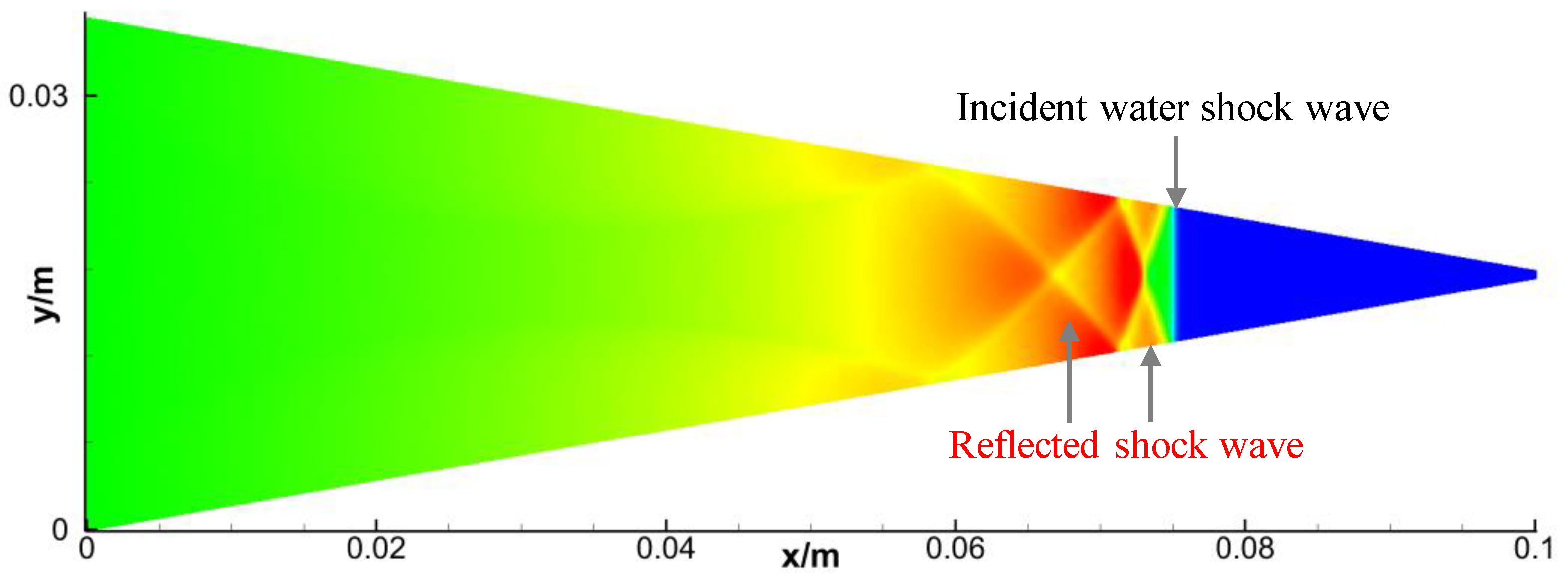
3.2. Validation of Pulse Hydraulic Fracturing

Pulse hydraulic fracturing is a key technology for improving the permeability of rock formations [7,24]. There are phenomena of propagation, reflection, and pressurization of pulse pressure waves in the pulse hydraulic fracturing. Accurately evaluating the peak pressure after pulse reflection is of great significance for evaluating the fracturing effect. Due to the difficulty of measuring the peak pulse pressure inside reservoirs experimentally, especially in fissures with small openings, it is particularly necessary to use simulation methods to obtain the peak pulse pressure inside the fracture. In addition, the existing simulation methods often use the low-precision or MAC methods, which either have severe dissipation and smoothing effects, or have severe dispersion and oscillation characteristics, making them unsuitable for the prediction of pulse peak pressure. In view of this, we derived the FVS formula and developed the FVS-WENO program based on Fortran language. Then, we adopted the FVS-WENO method to calculate and simulate the pulse supercharging process.

In order to demonstrate the superiority of the FVS-WENO format in pulse peak prediction, we conduct a series of simulations and comparisons. The simulation parameters are as follows: the length of the wedge-shaped structure is L = 0.1 m, the width of the left end is H = 0.03527 m, and the wedge angle is 20°. At the initial point, the water pressure inside the wedge-shaped structure is 1 MPa. Within the time interval of 0 < t < 1 ms, a constant water pressure p = 2 MPa is applied to the left boundary. The numerical calculation domain is a rectangular area (0 ≤ x ≤ 0.1 m, 0 ≤ y ≤ 0.03527 m) with grid number Nx = 1600, Ny = 564, and the time step meets the CFL condition. The wave speed is 1491 m/s. The immersed boundary (IB) method [25,26] is adopted to deal with the structure boundary. The detailed simulation parameters are listed in

Table 2. Simulation parameters of pulse hydraulic fracturing.

Parameter	Value
Wedge length/(m)	0.1
Wedge width/(m)	0.03527
Wedge angle/(°)	20
Initial pressure/(MPa)	1
Pulse pressure/(MPa)	2
Wave speed/(m/s)	1491
Grid number Nx	1600
Grid number Ny	564

.

For the boundary condition, it is assumed that the upper and lower walls are non-slip rigid walls, the second-order IB method is used for the treatment of the upper and lower walls. The introduction of the IB method can be found in reference [25,26]. In addition, it is necessary to ensure that the pressure gradient normal to the wall is equal to 0 and the wall velocity is equal to 0.

Results are shown in Figure 4 and Figure 5. At t = 0.02 ms, the pressure contours given by the MAC method have significant fluctuation, which indicate that there is an apparent dispersion effect. By comparison, a fluctuation of pressure contour given by the FVS-WENO method is not apparent. We also extract the pressure distribution on the middle-axis line marked by a red dashed line in Figure 4. By comparison, it was found that there is a severe dispersion phenomenon upstream of the discontinuity wave using the MAC method, where pressure oscillation exists, as shown in Figure 5. Obviously, from the perspective of predicting water pressure, the FVS-WENO format can provide more accurate prediction without false oscillation. Therefore, for the prediction of peak pressure in pulse hydraulic fracturing, the FVS-WENO method is more suitable. The above results also confirm that the proposed FVS formula is reliable and accurate for the simulation of weakly compressible water flow.

We also compared the topological shape of the reflected shock wave with the existing experimental data [27,28], as shown in Figure 6 and Figure 7. We found that the present simulation results based on the FVS-WENO method are consistent with the experimental observations. The captured shock wave agrees well with the experimental picture. Namely, the present numerical method can be used to simulate the evolution of water shock waves. These comparisons further confirm that the proposed FVS formula and developed program is suitable for the simulation of weakly compressible water flow.

3.3. Discussion

For the compressible gas medium, there is a mature FVS formula derived from the gas N-S equation and ideal gas equation of state. However, there is no FVS formula suitable for the compressible water medium. The main reason is that the water equation of state is more complex than the ideal gas equation of state. As a result, there is no publicly reported FVS model that can be referenced up to now. In this article, we consider the weak compressibility of the water medium and choose the linear model of the water state equation. Then, we show the splitting process of the flux vector and give a new FVS formula. Obviously, this original work is valuable in the simulation field of the weakly compressible water medium.

In this article, the FVS formula is derived based on the N-S equation. In fact, flux splitting is targeting the convective term of the N-S equation. The existence or absence of a viscous term does not affect the derivation of FVS expression. Therefore, it can also be understood that the FVS formula is derived from the Euler equation if ignoring the viscous term of the N-S equation.

Although we propose a new FVS expression for the simulation of the water medium, there is still much work to be done. The application scope of the proposed formula is mainly limited to a medium–low pressure range such as p < 1 GPa. For ultra-high pressure water p > 1 GPa, it is difficult to give an FVS formula because of the complexity of state equation, where the water state equation is described by an exponential form instead of a linear model. The exponential form of the state equation makes it difficult to give a universal FVS expression. These problems still need further research.

4. Conclusions

In this paper, we focus on the weakly compressible water flow and derive the FVS formula for the first time by combining the water N-S equation and linear state equation of the water medium. The proposed FVS expression lays an important foundation for the high-order numerical simulation of compressible water flow. This original work fills the gap in the simulation field of weakly compressible water flow.

To emphasize the innovative work, here we have rewritten the FVS formula and the detailed expressions are as follows:

$$\mathit{F}=\frac{\rho }{2}\left(\begin{array}{c}{\lambda }_2+{\lambda }_3\\ \left(u-a\right){\lambda }_2+\left(u+a\right){\lambda }_3\\ v{\lambda }_2+v{\lambda }_3\end{array}\right), \mathit{G}=\frac{\rho }{2}\left(\begin{array}{c}{\eta }_2+{\eta }_3\\ u{\eta }_2+u{\eta }_3\\ \left(v-a\right){\eta }_2+\left(v+a\right){\eta }_3\end{array}\right)$$

(16)

The eigenvalues of matrix A are λ₁ = u, λ₂ = u − a, and λ₃ = u + a. The eigenvalues of matrix B are η₁ = v, η₂ = v − a, and η₃ = v + a. The detailed derivation processes are given in Section 2. Based on Formula (16), many kinds of high-order algorithms can be used to simulate the weakly compressible water flow. In this article, we take the fifth-order WENO algorithm as an example to show that the proposed FVS formula is reliable and valuable for the high-precision simulation of weakly compressible water flow.

The proposed FVS formula provides the necessary conditions for the application of high-order algorithms such as the WENO scheme in the simulation field of compressible water. The traditional FVS formula is mainly suitable for the gas medium and could not be applied to the water medium. The proposed FVS formula is suitable for the water medium. The main reason is that the present FVS expression is derived from the N-S equation and state equation of water. We developed the computation program by combining the FVS formula and the WENO algorithm. The present numerical results agree well with the theoretical data and experimental data, which validate the reliability of the present FVS-WENO method in the simulation field of weakly compressible water flow.

References

1. Jia, X.Y.; Wang, S.S.; Xu, J. Nonlinear characteristics and corrections of near-field underwater explosion shock waves. Phys. Fluids 2022, 34, 046108. [Google Scholar] [CrossRef]
2. MacCormack, R.W. The effect of viscosity in hypervelocity impact cratering. AIAA Paper 1969, 40, 69–354. [Google Scholar]
3. Wylie, E.B.; Streeter, V.L.; Suo, L. Fluid Transients in Systems; Prentice Hall: Englewood Cliffs, NJ, USA, 1993. [Google Scholar]
4. Wan, W.Y.; Huang, W.R. Water hammer simulation of a series pipe system using the MacCormack time marching scheme. Acta Mech. 2018, 229, 3143–3160. [Google Scholar] [CrossRef]
5. Li, H.; Huang, B.X. Pulse supercharging phenomena in a water-filled pipe and a universal prediction model of optimal pulse frequency. Phys. Fluids 2022, 34, 106108. [Google Scholar] [CrossRef]
6. Li, H.; Huang, B.X. Pulsating pressurization of two-phase fluid in a pipe filled with water and a little gas. Phys. Fluids 2023, 35, 046111. [Google Scholar]
7. Li, H.; Huang, B.X.; Xu, H.H. The optimal sine pulse frequency of pulse hydraulic fracturing for reservoir stimulation. Water 2022, 14, 3189. [Google Scholar] [CrossRef]
8. Jiang, G.S.; Shu, C.W. Efficient implementation of weighted ENO schemes. J. Comput. Phys. 1996, 126, 202–228. [Google Scholar] [CrossRef]
9. Shu, C.W.; Osher, S. Efficient implementation of essentially non-osciallatory shock-capturing schemes. J. Comput. Phys. 1988, 77, 439–471. [Google Scholar] [CrossRef]
10. Toro, E.F. Riemann Solvers and Numerical Methods for Fluid Dynamics, 3rd ed.; Springer: Berlin/Heidelberg, Germany, 2009; pp. 87–89. [Google Scholar]
11. Li, Y.H. Equation of state of water and sea water. J. Geophys. Res. 1967, 72, 2665–2678. [Google Scholar] [CrossRef]
12. Shyue, K.M. An efficient shock-capturing algorithm for compressible multicomponent problems. J. Comput. Phys. 1998, 142, 208–242. [Google Scholar] [CrossRef]
13. Métayer, O.L.; Massoni, J.; Saurel, R. Modelling evaporation fronts with reactive Riemann solvers. J. Comput. Phys. 2005, 205, 567–610. [Google Scholar] [CrossRef]
14. Beig, S.A.; Johnsen, E. Maintaining interface equilibrium conditions in compressible multiphase flows using interface capturing. J. Comput. Phys. 2015, 302, 548–566. [Google Scholar] [CrossRef]
15. Li, X.J.; Zhang, C.J.; Wang, X.H.; Yan, H.H. Numerical study on the effect of equations of state of water on underwater explosions. Eng. Mech. 2014, 31, 46–52. (In Chinese) [Google Scholar]
16. Yu, J.; Pan, J.J.; Wang, H.K.; Mao, H.B. A γ-based model interface capturing method to near-field underwater explosion (undex) simulation. J. Ship Mech. 2015, 19, 641–653. [Google Scholar]
17. Zhang, A.M.; Li, S.M.; Cui, P.; Li, S.; Liu, Y.L. A unified theory for bubble dynamics. Phys. Fluids 2023, 35, 033323. [Google Scholar] [CrossRef]
18. John, D.; Anderson, J.R. Computational Fluid Dynamic: The Basics with Applications; McGraw-Hill, Inc.: New York, NY, USA, 1995. [Google Scholar]
19. Henrych, J. Explosion Dynamics and Its Applications; Science Press: Beijing, China, 1987; pp. 152–160. (In Chinese) [Google Scholar]
20. Wu, Q.; Wang, K.; Kong, D.C.; Zhang, J.Y.; Liu, T.T. Numerical simulation of subsonic and transonic water entry with compressibility effect considered. Ocean Eng. 2023, 281, 114984. [Google Scholar] [CrossRef]
21. Chakravarthy, S.R. The Split Coefficient Matrix Method for Hyperbolic Systems of Gas Dynamic Equations. Ph.D. Thesis, Iowa State University, Ames, IA, USA, 1980. [Google Scholar]
22. Steger, J.; Warming, R.F. Flux vector splitting of the inviscid gasdynamic equations with application to finite-difference methods. J. Comput. Phys. 1981, 40, 263–293. [Google Scholar] [CrossRef]
23. Bergant, A.; Simpson, A.R.; Vtkovsk, J. Developments in unsteady pipe flow friction modelling. J. Hydraul. Res. 2001, 39, 249–257. [Google Scholar] [CrossRef]
24. Zhai, C.; Yu, X.; Xiang, X.W.; Li, Q.G.; Wu, S.L.; Xu, J.Z. Experimental study of pulsating water pressure propagation in CBM reservoirs during pulse hydraulic fracturing. J. Nat. Gas Sci. Eng. 2015, 25, 15–22. [Google Scholar] [CrossRef]
25. Peskin, C.S. Flow patterns around heart valves: A numerical method. J. Comput. Phys. 1972, 10, 252–271. [Google Scholar] [CrossRef]
26. Ghias, R.; Mittal, R.; Dong, H. A sharp interface immersed boundary method for compressible viscous flows. J. Comput. Phys. 2007, 225, 528–553. [Google Scholar] [CrossRef]
27. Eliasson, V.; Mello, M.; Rosakis, A.J.; Dimotakis, P.E. Experimental investigation of converging shocks in water with various confinement materials. Shock Waves 2010, 20, 395–408. [Google Scholar] [CrossRef]
28. Wang, C.X.; Qiu, S.; Eliasson, V. Investigation of shock wave focusing in water in a logarithmic spiral duct, Part 1: Weak coupling. Ocean Eng. 2015, 102, 174–184. [Google Scholar] [CrossRef]
Figure 1. Water equation of state described by a linear model (7) which is consistent with the Tait model. Here the y-axis shows dimensional pressure which is computed by combining Equation (7) and the reference pressure pref = 1 MPa. The experimental data are from reference [15].
Water 15 03699 g001
Figure 2. Comparison of wave speed between the present simulation and theory.
Water 15 03699 g002
Figure 3. Comparison of water pressure for the water hammer case, (a) variation regularity of water head at the right endpoint of pipe, (b) variation regularity of water head at the midpoint of pipe. Here exp is the experimental data from [23].
Water 15 03699 g003
Figure 4. Comparison of water pressure distribution, (a) simulation results from the MAC method, (b) simulation results from the FVS-WENO method.
Water 15 03699 g004
Figure 5. Comparison of water pressure curves along the symmetry axis marked by the dashed line in Figure 4.
Water 15 03699 g005
Figure 6. Simulation results of water shock wave reflection in wedge-shaped structure based on the present FVS-WENO method. The red represents the high-pressure and the blue represents the low-pressure.
Water 15 03699 g006
Figure 7. Experimental photos of water shock waves’ reflection in wedge-shaped structure from reference [28].
Water 15 03699 g007