Climate Change Scenarios Reduce Water Resources in the Schuylkill River Watershed during the Next Two Decades Based on Hydrologic Modeling in STELLA

Abstract

The Schuylkill River Watershed in southeastern PA provides essential ecosystem services, including drinking water, power generation, recreation, transportation, irrigation, and habitats for aquatic life. The impact of changing climate and land use on these resources could negatively affect the ability of the watershed to continually provide these services. This study applies a hydrologic model to assess the impact of climate and land use change on water resources in the Schuylkill River Basin. A hydrologic model was created within the Structural Thinking Experiential Learning Laboratory with Animation (STELLA) modeling environment. Downscaled future climate change scenarios were generated using Localized Constructed Analogs (LOCA) from 2020 to 2040 for Representative Concentration Pathways (RCP) 4.5 and RCP 8.5 emission scenarios. Three regional land use change scenarios were developed based on historical land use and land cover change trends. The calibrated model was then run under projected climate and land use scenarios to simulate daily streamflow, reservoir water levels, and investigate the availability of water resources in the basin. Historically, the streamflow objective for the Schuylkill was met 89.8% of the time. However, the model forecasts that this will drop to 67.2–76.9% of the time, depending on the climate models used. Streamflow forecasts varied little with changes in land use. The two greenhouse gas emission scenarios considered (high and medium emissions) also produced similar predictions for the frequency with which the streamflow target is met. Barring substantial changes in global greenhouse gas emissions, the region should prepare for substantially greater frequency of low flow conditions in the Schuylkill River.

1. Introduction

As water demand increases to meet global population growth, water resources are simultaneously threatened by anthropogenic impacts to watersheds around the world, including land use and climate change. Water resources are essential to society and the economy, providing services including drinking water, irrigation, transportation, energy generation, and recreation. Water management policies are designed to allocate available water resources to meet the highest priority demands in a watershed, given uncertainty and variability in many factors, such as seasonal flow trends, droughts, floods, and groundwater levels. However, these factors are now vulnerable to a compounding uncertainty, the changing precipitation, evaporation, and temperature associated with climate change [1,2].

Increasing anthropogenic greenhouse gases in the atmosphere are driving changes in precipitation and temperature levels [3]. Moreover, changes in the frequency, intensity, and spatial patterns of precipitation are increasing the magnitude and frequency of extreme events such as floods and droughts [4]. The global mean surface temperature is projected to increase by 2.6 to 4.8 °C at the end of the 21st century under the Intergovernmental Panel on Climate Change’s RCP 8.5 emissions scenario, a comparatively high greenhouse gas emission scenario [3].

Compounding climate change impacts, land use and land cover changes alter hydrologic processes such as infiltration, groundwater recharge, base flow, and runoff in watersheds [5,6,7,8]. Increasing the area of impervious cover through urban development in a region will increase the amount of runoff and decrease the amount of water infiltrated to groundwater [9,10]. An increase in runoff increases the possibility of flooding and erosion.

Due to changes in population and land use as well as climate change, the gap between available water resources and demand is expected to require difficult tradeoffs [11,12]. Conventional water resource management practices rely on the assumption of stationarity and may not be adequate to overcome uncertainties related to the future availability of water resources and extreme events [13,14]. Previous work has been conducted on the impacts of climate change on water resources at the basin and sub-basin scale using several types of hydrologic models [15,16,17]. There is no single framework that is appropriate for all applications but rather a variety of modeling strategies that vary in their scope, complexity, transparency, and spatiotemporal detail. Research on a variety of modeling strategies and geographic regions is necessary so that appropriate options can be developed for the many different use cases.

This study examines the Schuylkill River, a key source of water supply for one of the largest cities in the United States, Philadelphia, and for many other communities in the densely populated southeastern area of Pennsylvania. The basin is increasingly subject to water stress [18]. The Schuylkill River Basin is important in its own right and provides a well-monitored watershed subject to substantial pressure from development and urbanization, for which a framework for jointly evaluating the impacts of climate change and urbanization can be developed and readily parameterized.

Prior research on the Delaware River Basin [19], which contains the Schuylkill River Basin, describes the probable shift in regional weather patterns and predicts that there will be more extreme weather events, with a more active Atlantic hurricane season and higher intensity storm events with short-duration, but severe, dry periods. This change may cause a potential increase in flood events and an increase in temperatures which will directly affect local evapotranspiration rates, thereby bringing about extended drought cycles.

Prior research has not examined the joint impact of climate and land use change on water resources for the Schuylkill Watershed. The possible effects of climate change on water resources differ within a region due to the unique characteristics and land use trends of each basin; therefore, these impacts need to be investigated on a local scale to develop holistic approaches to overcome uncertainties associated with the availability of water resources. Prior research of the full Delaware Watershed points to significant spatial variability in hydrological predictions [20]. Therefore, this localized study at the sub-watershed scale is necessary to develop a robust and resilient solution to the water resources management challenges and adaptive policies.

This study couples precipitation runoff models with stock and flow models of surface and groundwater resources using the STELLA mathematical modeling environment. The framework provides spatially detailed descriptions of evapotranspiration and surface water flow, while avoiding mechanistic models of vadose and saturated zone transport in favor of empirically estimated groundwater stocks and flows. The objective is to develop and evaluate a set of integrated models that provide water resource managers with the ability to explore scenarios with different estimates of future temperature, precipitation, and land use while avoiding unnecessary complexity and computational burden.

2. Materials and Methods

2.1. Description of Study Area

The Schuylkill River Watershed located in southeastern Pennsylvania encompasses nearly 5180 square kilometers and contains eleven counties (Figure 1). The Schuylkill River originates at its headwaters in Tuscarora Springs in Schuylkill County, and travels approximately 210 km to its mouth at the Delaware River in Philadelphia [21]. Flows in the Schuylkill are managed by regulating releases from the Blue Marsh Reservoir located roughly 105 km northwest of Philadelphia. The climate of the Schuylkill River Watershed is generally humid. The mean annual temperature in the watershed is 11 °C. The average temperatures during winter and summer are −1 °C and 22 °C, respectively [22]. The topography and elevation affect the precipitation trends in the watershed. The annual precipitation in the mountain regions in the watershed is 1150–1270 mm/yr and it decreases to 1092 mm/yr in the plain regions [21]. Flows of rivers and streams depend on the local precipitation rates within the Schuylkill River Basin. Evaporation is also an important factor affecting water availability in the basin. On average in Pennsylvania, 50% of annual precipitation is returned to the atmosphere through evaporation and transpiration by plants, 20% turns into stormflow and augments rivers and streams during rainfall and snowmelt events, and 30% recharges groundwater aquifers by infiltration [23]. Soil conditions vary in the watershed, with the predominant soil types being well drained and many areas have significant slopes. These conditions result in moderate runoff during wet weather in much of the basin [24]. Total withdrawals in the basin are divided into six categories: drinking water, power sector demand, agricultural demand, mining, industrial water demand, and others [25]. The percentage water consumption among sectors in the Schuylkill River Watershed is shown in

Table 1. Percentage of Water Consumption in Schuylkill River Watershed.

Sectors	Annual Average Withdrawals (m3/s)	Percentage of Water Consumption (%)
Power	9.34	41%
Drinking Water	7.02	31%
Agriculture	3.40	15%
Mining	1.59	7%
Industrial	0.91	4%
Others	0.48	2%

.

The primary land uses of the region have changed over the years, progressing from primarily agricultural to industrial due to vast natural resources including iron ore, hardwood, and river power. The discovery of vast coal sources in the northern headwaters made the Schuylkill River a primary mode of transportation. The industrial growth caused water pollution, habitat degradation, and hindered fish migrations [21]. Around 97–98% of Pennsylvania was forested land cover before colonial settlement. In the early 1990s, land use in the Schuylkill Watershed ranged from over 70% forest cover to less than 33% in agricultural and developed sections [21].

2.2. Hydrologic Model Equations

The Structural Thinking Experiential Learning Laboratory with Animation (STELLA) is an object-oriented, graphical modeling software package designed by Barry Richmond and commercialized by High Performance Systems (available at https://www.iseesystems.com/, accessed on 15 June 2023). This modeling environment was selected because STELLA has been widely applied to model water balances in biological, ecological, and environmental research studies [28,29,30]. Additionally, STELLA was selected in this study for its strength as a system dynamics approach which incorporates feedback loops between flows and stocks [31]. In this study, the STELLA modeling environment was used to code watershed management policies and reservoir operation rules to simulate observed streamflow of the Schuylkill River as well as its tributaries.

There are four watershed management policies related to streamflow conditions in the Schuylkill River Watershed including (1) Delaware River Basin Commission (DRBC) directed releases from Blue Marsh Reservoir, (2) minimum release criteria from Blue Marsh Reservoir, (3) drought demand restrictions in Pennsylvania, and (4) the consumptive use replacement policy for the Limerick Generation Station (LGS). The Blue Marsh Reservoir was programmed to simulate three watershed management policies defined in the Water Control Manual of Blue Marsh: (1) seasonal storage elevations, (2) flood control, and (3) conservation releases. DRBC-directed releases from Blue Marsh Reservoir were not included in the model since these releases are triggered by the streamflow conditions in the Delaware River. Twenty-seven nodes, representing existing USGS gages and confluences in the watershed, were programmed to simulate withdrawals and discharges. Wadesville and Bradshaw Reservoirs were programmed to simulate augmentation policies regarding LGS. Still Creek, Ontelaunee, and Green Lane Reservoirs are three additional reservoirs located in the watershed. They were omitted from the model due to the lack of historical inflow and reservoir storage data required to calibrate and validate simulation results.

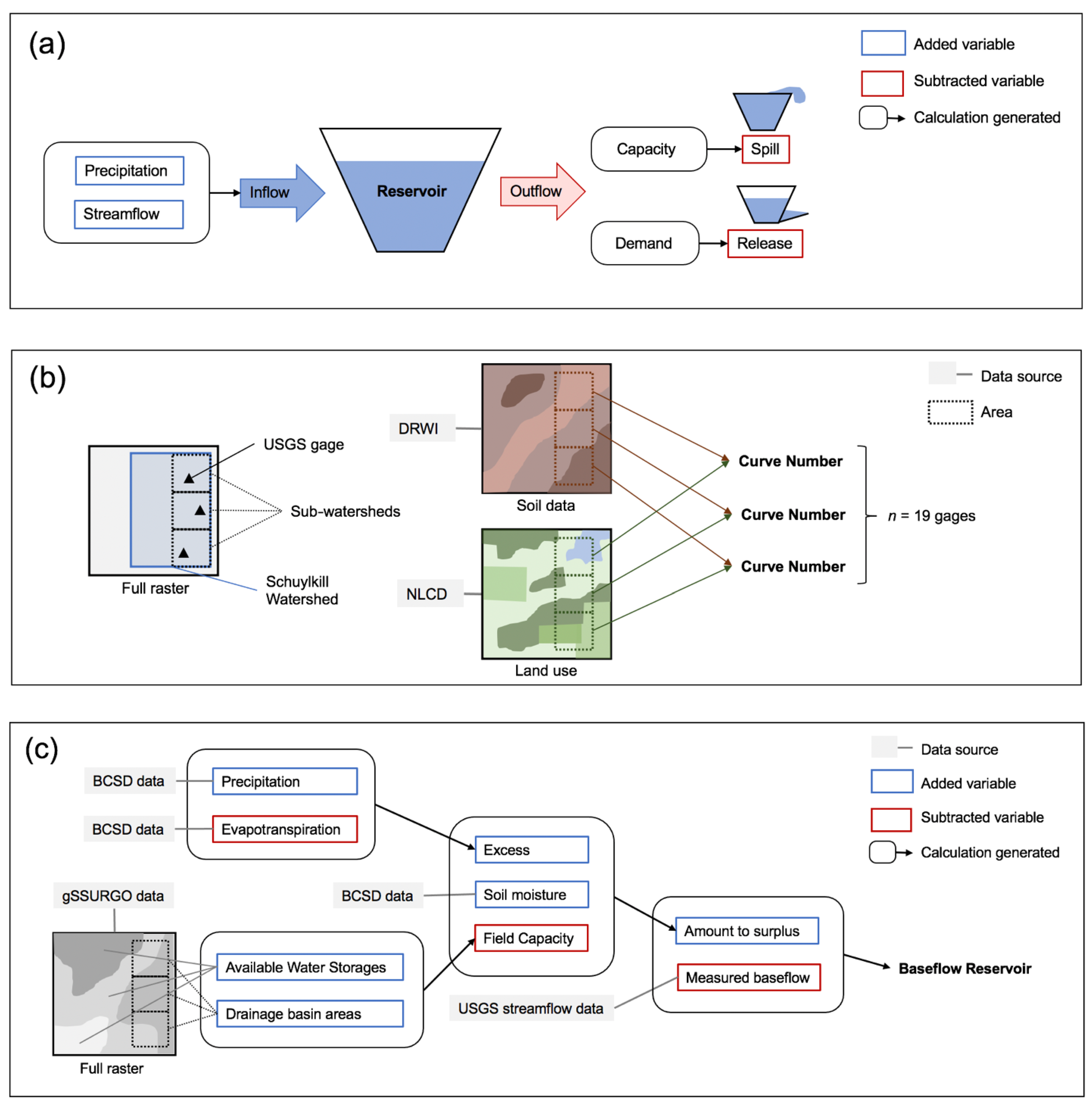
The primary concept of hydrologic modeling in STELLA ([32]; Equations (1)–(8)) is the continuity principle which requires conservation of the amount of water in a system, called a Reservoir (Figure 2a). Conservation of mass in a system is described by Equation (1), which defines the inflow and outflow for single time steps ($\mathrm{\Delta }t$) within a reservoir. STELLA automatically creates a continuity equation for mass balance for stocks based on inflows and outflows to stocks. Equation (1) calculates Reservoir Volume (V) (m³), based on inflows and outflows further defined in Equations (2) and (3), where SF = Streamflow and P = Precipitation. Inflow (I) represents water entering the reservoir, which is defined in Equation (2) as Streamflow (SF) (m³/day) plus Precipitation (P) (mm), normalized by reservoir area to account for the direct precipitation to the reservoir. Outflow (O) (m³/day) is water removed from the reservoir, which is defined in Equation (3) as the combination of Release (r) (m³/day), a controlled removal of water from a reservoir, and Spill (s) (m³/day), an overflow of excess water beyond storage and use.

$$V\left(t\right)=V\left(t-\mathrm{\Delta }t\right)+\left[I\left(t\right)\ast \mathrm{\Delta }t-O\left(t\right)\ast \mathrm{\Delta }t\right]$$

(1)

$$I\left(t\right)=SF\left(t\right)+P\left(t\right)$$

(2)

$$O\left(t\right)=r\left(t\right)+s\left(t\right)$$

(3)

V = Reservoir Volume (m³)

I = Inflow (m³/day)

SF = Streamflow (m³/day)

P = Direct precipitation to the reservoir (mm)

O = Outflow (m³/day)

r = Releases (m³/day)

s = Spill (m³/day)

To calculate Release (r) and Spill (s), Demand (D) (m³/day), the water utilized for drinking water and all other applications, is first defined as a function of Base Demand (b) (m³/day), the minimum water use, and Peaking Factor (p), a ratio of the maximum water use divided by average daily use (Equation (4)). Conditional statements are used to program controlled releases and excess spills from the reservoir (Equations (5) and (6)). In the first condition (Equation (5)), the amount of water removed as a controlled Release (r) is equal to Demand (D) if the Reservoir Volume (V) plus Inflow (I) is adequate to meet the specified demand. If sufficient resources are not available, Release (r) equals Reservoir Volume (V) at the current time step plus Inflow (I). Additionally, dumping of excess amounts of water as Spill (s) (Equation (6)) will only occur when the Reservoir Volume (V) plus Inflow (I) minus Release (r) is greater than the Capacity (C) (m³), defined as the maximum volume of storage possible within a reservoir. The spill calculation is not activated if the Capacity (C) is not exceeded.

$$D=b\ast p$$

(4)

$$r\left(t\right)=\left\{\begin{array}{c}D for V\left(t\right)+I\left(t\right)\ge D\\ V\left(t\right)+I\left(t\right) for V\left(t\right)+I\left(t\right)<D\end{array}\right.$$

(5)

$$s\left(t\right)=\left\{\begin{array}{c}V\left(t\right)+I\left(t\right)-r\left(t\right) for V\left(t\right)+I\left(t\right)-r\left(t\right)\ge C\\ 0 for V\left(t\right)+I\left(t\right)-r\left(t\right)<C\end{array}\right.$$

(6)

D = Demand (m³/day)

b = Base Demand (m³/day)

p = Peaking Factor

C = Capacity (m³)

The composite curve number method was used to approximate the amount of runoff produced based on predicted precipitation patterns in the area (Figure 2b). The runoff curve number is a single parameter, combining the effects of soil type, watershed characteristics, and land use [33]. The hydrologic soil data were derived from the Delaware River Watershed Initiative Soils raster dataset and the National Land Cover Database (NLCD) raster datasets. The ArcGIS software (available online: https://www.esri.com/en-us/arcgis/about-arcgis/overview, accessed on 15 June 2023) was used to integrate the data from both raster datasets. The Schuylkill River Watershed was divided into sub-watersheds based on the USGS streamflow gages considered for the study. The CN of each gage was calculated as an area-weighted average based on land use type and soil type corresponding to each drainage area in the ArcGIS software (see Appendix A 

Table A1. STELLA nodes with the corresponding USGS gages, drainage areas, and composite curve number calculated based on the most recent land cover dataset.

STELLA Node	USGS Gage Number	Drainage Area (km2)	Curve Number (2011)
Upper Perkiomen	01472198	98.4	71.79
Reading	01471510	813.3	74.30
Dublin	01472620	10.5	73.53
Skippack	01473120	139.1	77.03
Norristown	01473500	726.0	76.24
Schwenksville	01472810	141.5	76.11
Philadelphia	01474500	178.7	85.39
Little Schuylkill	01470500	259.0	69.39
Pottstown	01472000	470.1	73.12
Landingville	01468500	199.2	70.21
Graterford	01473000	472.2	72.58
Pottsville	01467500	138.3	68.38
Blue Marsh	01470960	453.2	74.79
Drehersville	01470000	204.9	68.80
Wissahickon	01474000	165.8	79.15
Tamaqua	01469500	111.1	68.74
Manatawny	01471980	74.1	72.17
Tulpehocken	01471000	93.2	75.57
Spangsville	01471875	147.4	71.91

—CN values). The depth of Runoff (Q), was calculated based on Precipitation (P), and S, which is the maximum potential of soil retention of water (Equation (7)), where S = (1000/CN-10).

$$Q\left(t\right)=\left\{\begin{array}{c}\frac{{\left(P\left(t\right)-I_a\right)}^2}{\left(P\left(t\right)-I_a\right)+S}\\ I_{a }=0.2S\\ 0 for P\le 0.2S\\ \frac{{\left(P\left(t\right)-0.2S\right)}^2}{P\left(t\right)+0.8S} for P>0.2S\end{array}\right.$$

(7)

Q = Runoff (mm)

P = Precipitation (mm)

S = Potential maximum retention after runoff begins

I_a = Initial abstraction (20% of S)

To account for groundwater resources in the study area, the streamflow sustained by groundwater, or baseflow, was estimated by incorporating the effects of available precipitation, potential evapotranspiration (water loss through evaporation and transpiration), soil moisture (water content of the soil), and field capacity (maximum water content held in the soil) (Figure 2c). Hawkins [34] presents a method for calculating the baseflow produced in an area at a monthly time step. This method was modified to calculate the baseflow available in a region at a daily time step to match the time step being used in the accompanying STELLA streamflow model ([34]; Equations (8) and (9)). The observed historical data for the available precipitation, the potential evapotranspiration, and the soil moisture datasets were obtained from the Bias-Correction Spatial Disaggregation (BCSD) hydrologic model available through ‘Downscaled CMIP3 and CMIP5 Climate and Hydrology Projections’ [35]. The potential evapotranspiration and the soil moisture data were only available at a monthly time step and were converted to match the STELLA model’s daily time step by dividing the monthly values by the number of days in each respective month.

Field Capacity was calculated for each drainage area associated with the USGS streamflow gages included in the study. The available water storage values, derived from the amount of water stored in the top 0–150 cm layer of soil within the Schuylkill River Watershed, were obtained from the Gridded Soil Survey Geographic (gSSURGO) website as a raster dataset. Historical data allow overall water storage in the basin to be estimated by previous studies, but the hydrologic model developed here required smaller scale water storage values to understand how changes in land use would affect future hydrology. The available water storage values for each of the USGS gages were obtained by assigning the water storage in the watershed to different individual drainage areas in proportion to the drainage area size. The raster dataset was processed in ArcGIS to produce an attribute table with data depicting the type of soils present, their corresponding Available Water Storages, and Hydrologic Group Dominant Conditions (

Table 2. Attribute table depicting data used for Field Capacity calculation. The ‘Count’ column lists the number of cells that contain the cell value and the values in the ‘Available Water Storage’ (AWS) column represent the amount of water stored within the 0–150 cm storage layer based on the soil type and infiltration capacity.

Count	Map Unit Name	Available Water Storage 0–150 cm—Weighted Average (cm/m)	Hydrologic Group—Dominant Conditions
9048	Andover–Buchanan gravelly loams, 3 to 8 percent slopes	14.28	D
8388	Andover–Buchanan gravelly loams, 0 to 8 percent slopes, extremely stony	14.32	D
21,275	Bedington–Berks complex, 3 to 8 percent slopes	13.82	A
15,685	Bedington–Berks complex, 8 to 15 percent slopes	13.22	A
3378	Berks–Bedington complex, 15 to 25 percent slopes	11.48	B
3861	Berks–Weikert complex, 0 to 3 percent slopes	7.61	B
282,303	Berks–Weikert complex, 3 to 8 percent slopes	7.35	B

).

Field Capacity (FC) was calculated using the Available Water Storage (AWS), defined as the weighted average water stored in the top 0–150 cm layer of soil, and the calculated Area (A) of each soil category. The Field Capacity values for each soil type were aggregated to obtain the cumulative Field Capacity for the whole drainage area and then converted from cm to mm. The Field Capacity values generated for all the gages with the hydrologic STELLA model can be found in Appendix A 

Table A2. Field Capacity values.

Gage Name	USGS Gage Number	Field Capacity (mm)
Upper Perkiomen	1472198	166.72
Reading	1471510	129.15
Dublin	1472620	138.01
Skippack	1473120	114.71
Norristown	1473500	130.38
Schwenksville	1472810	121.07
Philadelphia	1474500	84.61
Little Schuylkill	1470500	116.56
Pottstown	1472000	154.18
Landingville	1468500	102.43
Graterford	1473000	153.80
Pottsville	1467500	107.28
Blue Marsh	1470960	148.04
Drehersville	1470000	115.21
Wissahickon	1474000	111.94
Tamaqua	1469500	133.55
Manatawny	1471980	158.58
Tulpehocken	1471000	139.96
Spangsville	1471875	185.42

.

Using the parameters previously described, we employed a methodology derived from Hawkins [34] to calculate baseflow in the region at a daily time step. Baseflow contributes to streamflow whenever precipitation saturates and then exceeds the field capacity (or maximum soil moisture storage) of the soil. Excess (E) precipitation was calculated as the difference between Precipitation (P) and PE (Potential Evapotranspiration) (Equation (8)). If the Excess (E) was positive, it resulted in replenishment of Soil Moisture (SM) up to its maximum capacity, or Field Capacity (FC). If Excess (E) was negative, then Soil Moisture (SM) was calculated as presented in Equation (9), where t indicates the current day and FC is the Field Capacity. For the time steps where Excess (E) was positive and SM (t) was at field capacity, then the water depth (mm) contributing to baseflow in the region, or the Surplus (L), was estimated based on the Excess Precipitation (E), the Field Capacity (FC) and the Soil Moisture (SM) (Equation (10)). The recorded Soil Moisture was used for SM at the first timestep [34].

$$E\left(t\right)=P\left(t\right)-PE\left(t\right)$$

(8)

$$SM\left(t\right)=\left\{\begin{array}{c}SM\left(t-\mathrm{\Delta }t\right)+E\left(t\right)-FC\left(t\right) for E\left(t\right)>0\\ SM\left(t-\mathrm{\Delta }t\right)+\frac{E\left(t\right)\ast SM\left(t-\mathrm{\Delta }t\right)}{FC\left(t\right)} for E\left(t\right)\le 0\end{array}\right.$$

(9)

$$L\left(t\right)=E\left(t\right)+SM\left(t-\mathrm{\Delta }t\right)-FC\left(t\right)$$

(10)

$$IF L\left(t\right)<0, L\left(t\right)=0$$

(11)

E = Excess Precipitation (mm)

P = Precipitation (mm)

PE = Potential Evapotranspiration (mm)

SM = Soil Moisture (mm)

FC = Field Capacity or maximum soil moisture (mm)

L = Surplus (mm)

The Surplus (L) (mm) accumulated in a hypothetical reservoir which was built into the model for every node. Total water depth (mm) available as Baseflow (B) (Equation (12)), is based on the estimated baseflow over time and X, the percentage of Baseflow Discharge removed from the accumulation reservoir (L). Baseflow rates are specific to each node and adjusted based on the historical streamflow behavior.

$$B\left(t\right)=X\ast L\left(t\right)$$

(12)

X = Baseflow Discharge rate (%)

B = Baseflow (mm)

The final step was calculating Streamflow (SF) at each node, which is the sum of Runoff generated after precipitation events (Q) and contribution of Baseflow (B) at each node multiplied by the corresponding Drainage Area (DA) (km²) (Equation (13)). Conversion factors are included in the modeling environment, yielding Streamflow (SF) in m³.

$$SF\left(t\right)=\left(Q\left(t\right)+B\left(t\right)\right)\ast DA$$

(13)

Q = Runoff generated in the drainage area (mm)

B = Baseflow (mm)

DA = Drainage area (km²)

SF = Streamflow (m³)

2.3. Hydrologic Model Validation

Our model calibration process involved modifying model parameters to generate a good reproduction of historical observations in the study area. Daily observed streamflow data from 2007 to 2008 were compared with the simulated streamflow data. The baseflow discharge rate (X) was manually adjusted for every node in the STELLA model to minimize the difference between the simulated and observed streamflow. In Appendix A,

Table A3. STELLA nodes with the corresponding USGS gages, baseflow rates, and initial abstraction values.

STELLA Node	USGS Gage Number	Percentage of Baseflow Discharge (X) (%)
Upper Perkiomen	01472198	5.6
Reading	01471510	11.5
Dublin	01472620	14.5
Skippack	01473120	1.5
Norristown	01473500	15.7
Schwenksville	01472810	25.1
Little Schuylkill	01470500	14.4
Pottstown	01472000	1.5
Landingville	01468500	10.0
Graterford	01473000	59.5
Pottsville	01467500	15.1
Blue Marsh	01470960	1.4
Drehersville	01470000	34.3
Wissahickon	01474000	15.2
Tamaqua	01469500	10.7
Manatawny	01471980	1.5
Tulpehocken	01471000	59.0
Spangsville	01471875	5.8

includes the adjusted parameters and corresponding gages. Once the model base flow rates were calibrated, the model ran from 2008 to 2010 with the calibrated parameters to validate the consistency of these parameters.

To verify the simulated storage level of Blue Marsh Reservoir, the observed reservoir elevation data were gathered from USGS gage 01470870 Blue Marsh Lake for three years from 2007 to 2010. The model predicts the reservoir storages as a volume rather than an elevation. For verification purposes, the observed elevation data were converted to the storage values with the help of an elevation-storage curve. To estimate the relationship between observed elevation and storage values, annual average elevation and storage data for Blue Marsh Reservoir were downloaded from the USGS website. This dataset is available for every water year and can be found in the annual Water Data Reports. Regression analysis was applied to the downloaded data and the relationship between observed elevation and storage values was estimated. Once the relationship between elevation and storage values was determined, the daily observed elevation data were converted to the storage values to be compared with the predicted storage values.

2.4. Future Climate Scenarios

The baseline model simulated streamflow in the Schuylkill River given existing water management policies and a historical streamflow record from 2007 to 2010 using a daily time step and the mass balance approach. The purpose of the baseline scenario was to validate the model’s prediction of streamflow against measured streamflow at specific USGS gages. After validation, the baseline model was run to simulate streamflow from 2020 to 2040 while varying CO₂ emission levels (2 scenarios), local climate change parameters (12 scenarios) and land use change (3 scenarios) in order to assess the water resource availability beyond the historical record.

Climate projections were obtained from the General Circulation Models (GCMs), numerical models that represent the physical processes in the atmosphere, ocean, cryosphere, and land surface and provide estimates for future climate conditions based on the historical climate conditions and greenhouse gas emissions [36]. GCMs forecast climate projections at large scales with coarse spatial and temporal resolution. The availability of surface water resources is mostly driven by local precipitation, temperature, and evapotranspiration, and therefore, high spatial resolution of these climate parameters is imperative. For this reason, climate predictions need to be downscaled to a finer spatial resolution on a sub-watershed level to account for accurate regional topography and climatic conditions [37].

Two methods were considered to downscale the GCMs to a sub-watershed resolution. The first method was modeling future non-stationary precipitation through a stochastic simulation of a non-stationary hourly precipitation series using monthly GCM temperature [38]. This method aims to project the future climate conditions based on historical conditions in a given area. Although this method was successful in prior studies for areas with sufficient information, it is not applicable in areas with gages that do not record enough data. For this study area, the downscaled data using this approach were only available at the gages in metropolitan areas, which could not be used as a representative precipitation profile for the entire watershed as this would counteract our objective of studying the local effects of climate change in different parts of the watershed.

Therefore, this study instead applied the second approach to downscaling climate projections, the Localized Constructed Analogs (LOCA) method. LOCA approximates the regional effects of climate change based on the systematic historical effects of topography on the local weather in a region. The LOCA downscaled climate projections provide temperature and precipitation data for a gridded model with a resolution of 6 km (3.7 miles). LOCA uses data from 32 coarse-resolution global climate models (GCMs) from the Climate Model Intercomparison Project, version 5 (CMIP5) archive and aims to preserve the regional effects as well as future climate conditions predicted by the GCMs simultaneously [37]. The LOCA methodology is able to reproduce existing climatological data with high accuracy (root mean squared error of roughly 2%, [39]). For our LOCA approach, historical data from the period 1950–2005 were used. Soil moisture content was computed using high resolution daily precipitation and minimum and maximum temperature as inputs in a single land surface/hydrology model called the Variable Infiltration Capacity (VIC) model. The systematic errors from the GCMs were removed through bias correction performed prior to downscaling the data. [40].

The LOCA-downscaled data were then used to model hydrologic conditions in the future. Two future climate projections were run, one using medium (Representative Concentration Pathway (RCP) 4.5) and one using high (RCP 8.5) greenhouse gas and aerosol emissions scenarios. RCP 4.5 (1.7–3.2 °C moderate warming) results from emissions peaking around 2040, and RCP 8.5 (3.2–5.4 °C extreme warming) results from emissions continuing to rise during the 21st century. Our resulting dataset includes daily precipitation, evapotranspiration, and soil moisture data from 2020 to 2040 for six General Climate Model (GCM) outputs for each of the two emission scenarios (RCP 4.5 and 8.5), for a total of 12 possible climate change conditions (

Table 3. Description of the General Circulation Models (GCMs) used to project future climate scenarios.

	GCM-1	GCM-2	GCM-3	GCM-4	GCM-5	GCM-6
GCM Name	ACCESS	BCC-CSM	BCC-CSM-1-1-m	CanESM 2	CCSM 4	CESM 1-BGC
Resolution	1.25° × 1.88°	2.8° × 2.8°	2.8° × 2.8°	2.79° × 2.81°	3.75° × 3.75°	0.94° × 1.25°
Full Name	ARC Centre of Excellence for Climate System Science	Beijing Climate Center Climate System Model	Beijing Climate Center Climate System Model	Canadian Earth System Model	Community Climate System Model	Community Earth System Model version 1.0 with Biogeochemistry
Components	Forcings: Solar, volcanic, stratospheric aerosol, anthropogenic aerosol, emissions, greenhouse gas	4 models: atmospheric, land-surface, oceanic, sea-ice	4 models: atmospheric, land-surface, oceanic, sea-ice	Models: atmosphere- ocean; land- vegetation	4 models: atmospheric, land-surface, oceanic, sea-ice	Models: Terrestrial carbon–nitrogen; ocean biogeochemistry
Proceeding GCMs		Follows CCSM2	Follows BCC-CSM		Subset of CESM1

).

2.5. Future Land Use Scenarios

To assess the impact of land cover change on water resources, future land cover and land use change projections were incorporated into the STELLA model through the composite curve number method. To estimate land use change in the future, population growth trends were used as a proxy for increasing impervious areas. The historical population growth rates were obtained from the United States Census Bureau Database [41]. The future population growth rates for each of the counties within the Schuylkill River Watershed were based on the Pennsylvania population projections 2010–2040 prepared by the Center for Rural Pennsylvania (

Table 4. Trends and forecasts of population growth rates.

County	Historical Population Growth (2000–2010)	Future Population Growth (2010–2040)
Berks	1.50%	20.30%
Bucks	0.50%	1.50%
Montgomery	3.30%	17.20%
Philadelphia	3.60%	21.70%
Schuylkill	−3.90%	12.10%

). These percentages were projected based on the base population, fertility rates, survival rates and the migration rates from within and outside the country [42].

Scenarios for cumulative change in impervious cover were developed for all the counties in the Schuylkill River Watershed for three growth scenarios: the As-is Scenario, Sprawl Growth Scenario, and the Smart Growth Scenario (

Table 5. Cumulative change in impervious cover in the three scenarios for all the counties in the Schuylkill River Watershed.

County	Historical Change in Impervious Cover (2001–2011)	As-Is Scenario (Historical Trends Projected into Future) (2010–2040)	Sprawl Growth Scenario (25% More Impervious Area than As-Is Scenario) (2010–2040)	Smart Growth Scenario (25% Less Impervious Area than As-Is Scenario) (2010–2040)
Berks	0.74%	10.05%	12.56%	7.54%
Bucks	1.92%	5.76%	7.20%	4.32%
Montgomery	0.60%	3.14%	3.93%	2.36%
Philadelphia	0.19%	1.12%	1.40%	0.84%

). For the As-is Scenario, the growth rates were based on historical trends in population growth and change in impervious cover. These values were obtained by scaling the historical population growth and change in impervious cover to the forecasted population growth rates for 2010–2040. Secondly, the Sprawl Growth Scenario was incorporated to forecast the change in impervious areas in cases where the urbanization rates would outpace the growth of the population [43]. The rates for the scenario were calculated by increasing the rates calculated for the As-is Scenario by 25%. Finally, the Smart Growth Scenario was incorporated to forecast the change in impervious areas in cases where the implementation of conservation trends would dampen the process of urbanization. The rates for this scenario were calculated by decreasing the rates calculated for the As-is Scenario by 25% [44].

The drainage areas for each of the gages incorporated into the STELLA model were divided into their respective counties. The drainage areas associated with each of the gages were cropped in ArcGIS, resulting in a unique attribute table for every gage. Based on the rates calculated for the specific gage, the attribute table was adjusted according to the projected land use conditions. The raster cells classified as ‘Low Intensity Residential’, High Intensity Residential’, ‘Developed, Medium Intensity’ and the ‘Developed, High Intensity’, land cover types including impervious area, were increased by the projected percentages for each of the land use change scenarios. These rows collectively accounted for the impervious area in the drainage area associated with the gage. The increase in urban area was subtracted from the ‘Deciduous Forest’, ‘Evergreen Forest’, ‘Pasture/Hay’ and the ‘Row Crops’ classes which account for the forested and agricultural areas. In all cases, the increase in impervious areas corresponded to a decrease in the areas associated with the forest and agriculture land use types, with the loss distributed evenly between the agricultural and forested land use areas.

3. Results

3.1. Hydrologic Model Validation

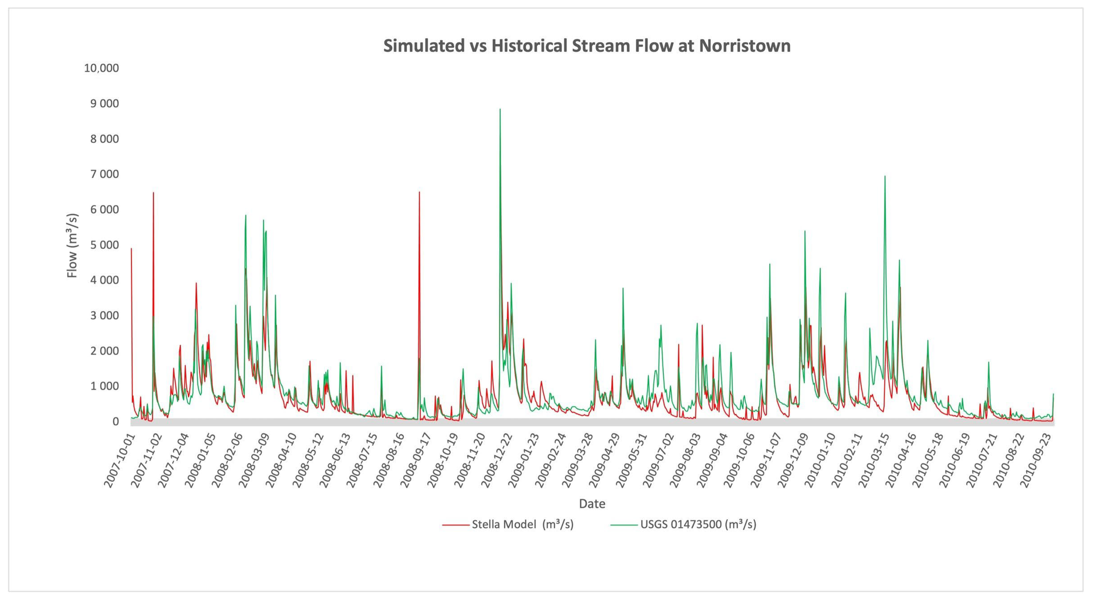
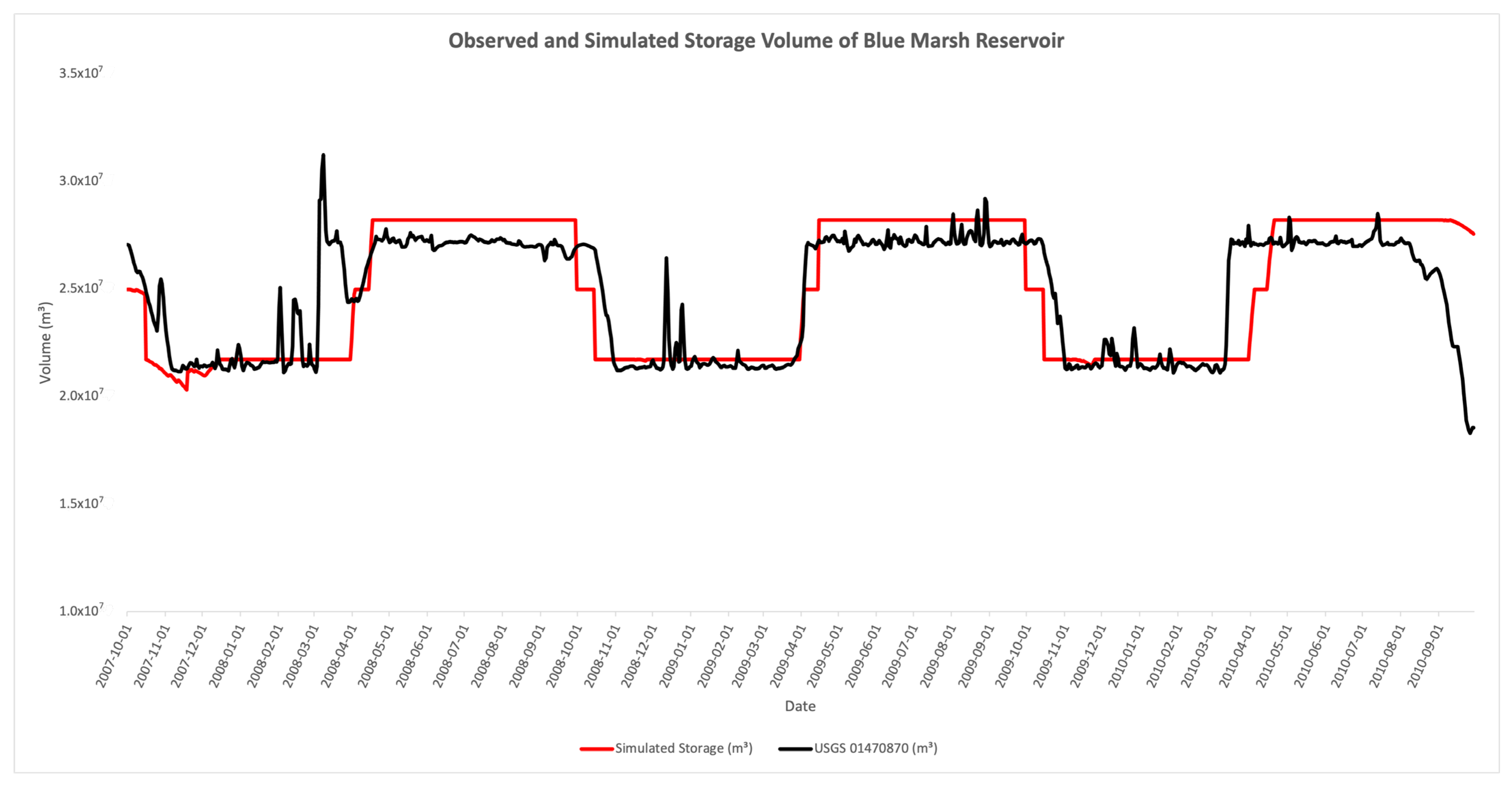
A comparison of daily observed streamflow data from 2007 to 2010 at one of the gages and our simulated flow levels is shown in Figure 3. Additional validation was provided by comparing the observed reservoir elevation data collected at the USGS gage 01470870 Blue Marsh Lake with our simulated levels for three years from 2007 to 2010 (Figure 4).

Further, statistical parameters, the including root mean square error (RMSE), coefficient of determination (R²), Nash–Sutcliffe efficiency (NSE), and Mean Absolute Percentage Error (MAPE), were employed to analyze the performance of our model (

Table 6. Statistical analysis of the modeled and observed streamflow in Norristown, and reservoir elevation at Blue Marsh. October 2007–2008 was used as the calibration period and October 2008–2010 was used as the validation period.

Norristown		Blue Marsh
Calibration (October 2007–2008)
RMSE	603.42	RMSE	1,891,819.24
R2	0.59	R2	0.65
NSE	0.53	NSE	0.46
MAPE	49.26	MAPE	4.83
Validation (October 2008–2010)
RMSE	566.08	RMSE	1,995,865.83
R2	0.58	R2	0.62
NSE	0.69	NSE	0.49
MAPE	43.80	MAPE	5.18

).

The graphs in Figure 3 and Figure 4 show reasonably good qualitative agreement between the observed and modeled streamflow at Norristown as well as between the simulated and observed storage levels for Blue Marsh Reservoir. For both the calibration and the validation periods, the R² values (Table 6) are moderate (0.59 for Norristown and 0.65 for Blue Marsh for the calibration period, and 0.58 for Norristown and 0.62 for Blue Marsh for the validation period), which are values considered acceptable by Moriasi et al. [45]. The NSE values in Table 6 are >0, which is generally viewed as acceptable for daily data [45]. The mean absolute percentage error of 44% for Norristown in the validation period highlights that the model is not precise in predicting daily peak streamflows. However, the mean absolute percentage error of 5.2% for Blue Marsh in the validation period indicates that the model performs better in capturing the annual fluctuations in reservoir levels. It should be noted that this model is working on a daily timestep. Simulating daily hydrological flow patterns on short timesteps is inherently challenging, given the intricate nature of hydrologic processes. The model sometimes offsets peak flows by a day, resulting in substantial errors despite capturing the qualitative pattern of streamflow. The figures illustrate that the model generally captures the system’s behavior, effectively depicting long-term trends and proving valuable outputs for long-term scenario assessment.

3.2. Future Climate Scenarios

Our model simulated water resource data over twenty years, from 2020 to 2040, with future climate data projected from twelve GCMs, under two emission scenarios (RCP 4.5 and RCP 8.5), and three land use change scenarios. To analyze the availability of water resources, we selected the stream gages in closest proximity to Philadelphia Water Department (PWD) intakes. In the Schuylkill River Watershed, no gage is located immediately upstream of the Water Department intakes. Therefore, Norristown, the nearest upstream gage, located ten miles upstream of the Philadelphia water intakes, was selected to assess the availability of water resources. To interpret the availability of future water resources in the Schuylkill River Watershed, flow targets were employed. Flow targets or streamflow objectives indicate the minimum amount of water desired at a specific location.

The historical streamflow objective for Norristown was based on the period from 1990–2010. The flow target for Norristown includes the maximum potable water demand for PWD, demand for the fish passage operation at Fairmount Dam, and a safety factor. At Fairmount Dam in Philadelphia, 2.83 m³/s is required to operate the fish ladder, and this is expected to continue given the ecological benefits provided by the ladder [12]. The maximum projected water demand for PWD was estimated to be 8.07 m³/s. In addition to the maximum potable water demand and fish passage operational demand, a 2.83 m³/s safety factor was added to the target flow. In total, the historical streamflow objective for Norristown is 13.73 m³/s (Hesson, 2013). Based on the projected population for Philadelphia County, the maximum PWD potable water demand was estimated to increase to 8.24 m³/s by 2040. In total, the projected streamflow target for Norristown was estimated as 13.90 m³/s by 2040.

The streamflow values from 2020 to 2040 under the twelve different climate change scenarios were compared with the flow target at Norristown to yield the total number of days when the streamflow at Norristown falls below the streamflow objective (13.90 m³/s) (

Table 7. Percentage of days in the period of 2020–2040 when the streamflow objectives are met at Norristown.

Historical Streamflow Availability	89.8%
	Emission Scenarios
GCM Inputs to STELLA	RCP 4.5	RCP 8.5
GCM-1	70.2%	75.0%
GCM-2	76.6%	75.4%
GCM-3	76.9%	75.6%
GCM-4	67.7%	67.2%
GCM-5	74.3%	75.1%
GCM-6	74.3%	74.7%

). The results show water resources availability for the Schuylkill River Watershed with each future climate change scenario as well as the availability of water resources for the last twenty years of the historical streamflow simulation period. The results show that 89.8% of the days in the historical period of 1990–2010 met the streamflow objectives at Norristown. For the predicted flows, 67.7–76.9% of the days in the period from 2020–2040 meet the streamflow objectives under the RCP 4.5 emission scenarios, and 67.2–75.6% of the days in the specified time period meet the streamflow objectives under the RCP 8.5 emission scenarios in the Schuylkill River Watershed. Compared with the historical period, the number of days each year failing to meet the target could increase by as much as 22.6% under the most extreme scenario, suggesting a need for revised water management protocols. Confidence intervals for the proportion of days meeting the streamflow objective are +/−1% for a 95% confidence level. Hence, in Table 7 values should differ by more than 2% to be considered significantly different. The modeled scenarios are all distinct from the historic value of 89.8%, although not necessarily from each other.

3.3. Future Land Use Scenarios

Land cover in the Schuylkill River Watershed includes forested lands, agricultural areas, and urban areas. The upper northwestern part of the watershed is primarily forested, with the agricultural areas being prevalent mainly in the middle and lower portions of the watershed, as well as in the northern Berks County region. The most densely urban areas are located around the cities of Philadelphia and Reading [21]. The land cover percentages of forested, agricultural, and urban areas in the watershed are 41%, 29% and 27%, respectively [14].

The values of future population growth in the Schuylkill Watershed are significantly higher than the historical population growth. Almost 90% of the population increase within the state is projected to be in urban counties, and all of the counties in the Schuylkill Watershed are classified as urban. Out of the five counties, Berks, Montgomery and Philadelphia counties are projected to have a 15.1% or greater increase in population, with Bucks and Schuylkill counties projected to have a population increase of 0–15.0% [42]. The expansion of impervious areas in watersheds is responsible for decreasing the infiltration capacity of land cover, and therefore, increasing the amount of runoff. Three land-use change scenarios were explored, as presented in

Table 8. Curve numbers corresponding to land use change scenarios.

Gage Name	Historical CN	As-Is Scenario Curve Number	Sprawl Growth Scenario Curve Number	Smart Growth Scenario Curve Number
Reading	74.30	74.60	74.67	74.52
Little Schuylkill	69.39	69.53	69.55	69.49
Blue Marsh	74.79	74.98	75.03	74.94
Manatawny	72.17	72.37	72.39	72.30
Tulpehocken	75.57	76.02	76.13	75.91
Spangsville	71.91	72.01	72.04	71.99
Upper Perkiomen	71.79	71.84	71.86	71.83
Skippack	77.03	77.23	77.30	77.19
Norristown	76.24	76.43	76.48	76.38
Schwenksville	76.11	76.26	76.30	76.22
Pottstown	73.12	73.25	73.28	73.22
Graterford	72.58	72.65	72.67	72.64
Dublin	73.53	73.57	73.58	73.56
Philadelphia	85.39	85.58	85.63	85.53
Wissahickon	79.15	79.25	79.28	79.23

: an “as-is” scenario in which land use change follows historical trends, a scenario with increased urban sprawl and a scenario of smart growth. The impact of the land use change scenarios on water resources in our model for the time period 2020–2040 was found to be insignificant (Table 8).

4. Discussion

This study evaluated scenarios that could result in a reduction in water resource availability in the Schuylkill River Watershed during the next twenty years. Under these scenarios, there is a substantial increase in the frequency with which flow targets in the Schuylkill River are not met. Under the most extreme climate scenario, as many as 82 additional days each year may fall below the streamflow target. Based on our model parameterized for the local watershed, the climate changes impact of intensifying precipitation drove much of the estimated reduction in streamflow rather than changes in land use. Potential evapotranspiration was reasonably similar across scenarios. Finally, there was little difference in the impacts of the RCP 4.5 and RCP 8.5 scenarios, which represent medium- and high-emissions pathways, respectively. For the study period, the maximum difference in frequency of achieving streamflow targets found between the two emission scenarios was 4.9%. The low impact of emissions and land use development scenarios in this watershed on changing water supply indicates that even large efforts for land use management or emissions reduction policy may not eliminate the possibility for significantly reduced streamflow.

The results of this study generally agree with a number of other studies of North America which predict a decline in precipitation events during warm seasons, causing more frequent low streamflow conditions and increases in temperature, which may in turn also increase the amount of water loss due to evaporation from lakes and reservoirs [13,46,47]. For example, Christensen et al. [16] simulated climate change impacts on streamflow in the Colorado River basin and found that with business-as-usual greenhouse gas emissions, the frequency of achieving Glen Canyon Dam release targets would drop from 92% historically to 59–72% during 2010 to 2098, causing a significant decrease in hydropower output. However, not all studies find increased water stress. Zhang et al. [48] simulated hydrologic processes using the Soil and Water Assessment Tool (SWAT) model under climate change scenarios for the Xin River basin in China and predicted that while low streamflow conditions will follow historical patterns, high streamflow conditions will increase drastically in the 21st century.

No prior published studies have modeled the near-term climate change impacts on the hydrology of the Schuylkill Watershed. However, prior studies have modeled climate change impacts on the regional hydrology of the Delaware Basin, which contains the Schuylkill River. Hawkins & Woltemade [20] created a hydrologic model with a coarse spatial resolution (~12km grid cells) of the full Delaware Basin and predicted precipitation increases of 8–16% by 2080–2099, runoff increases, and decreases in soil moisture in most areas. Hawkins & Woltmade did not forecast future streamflows or days of water stress, and hence, their results cannot be directly compared with the findings of this study [20].

In the upcoming decades, adjustments to watershed management policies will need to account for climate change. For example, one possible policy could be the application of a reservoir hedging mechanism to balance reservoir targets with streamflow objectives as water availability declines [20]. In the Schuylkill Watershed, this could involve revised reservoir management rules that would allow releases from Blue Marsh Reservoir to meet the flow targets. However, negative outcomes of this approach would include the potential impacts on recreational opportunities that currently occur at the reservoir. In addition, the use of resources stored in the Blue Marsh Reservoir to meet a flow target on a given day necessarily raises the potential risk that such resources would not be available in a future time of greater need. As the region’s available water resources may be altered in the coming decades, policy mechanisms that address these local climate change impacts are essential.

The application of our results for policy must consider the limitations of the model within the context of this study. Predictions of precipitation under climate change are subject to substantial uncertainty inherent in GCMs, RCPs and hydrologic models [49]. During the next century in this region, other models predict increasing winter precipitation [20], showing that climate models may produce results showing complex trends in seasonality, with impacts on both the central tendency and variability in future water availability. Additionally, updated policies including the Blue Marsh Reservoir operational rules and watershed management would shift the model results. Changes in these factors would significantly alter the projected water resources. Another limitation of the model is that it does not account for green infrastructure. Urban areas of the Schuylkill Watershed have incorporated extensive plans for improving green infrastructure and stormwater best management practices [50]. Future research should incorporate existing and proposed green infrastructure plans into the land use calculations for a more accurate representation of stormwater management.

The next steps of research with this model should include improvements to the processes used for obtaining the future climate and land use projections. Future research should investigate alternative rainfall-to-runoff calculation methods to optimize the runoff calculation process and compare this modeling approach with other hydrologic models in a model ensemble comparison. The impacts of land use change on specific soil types were not examined in our model. Expanded development might occur on high infiltration soils which may dominate the hydrological functioning of the watershed [11]. Therefore, the next steps could involve calculating the curve numbers for a “worst-case scenario” where a majority of the developed area would be added on soils with high infiltrations rate to examine if this scenario would cause land use changes to have a significant impact on water resources over time. Finally, future models could separate population trends by location in the watershed. By assessing the population growth patterns cell-by-cell within a gridded model, results could account for regional differences between counties and provide a higher spatial resolution. With county-level trends, management could target locations where land use and population growth matter most.

5. Conclusions

Our application of STELLA for hydrologic modeling of the Schuylkill Watershed predicted reductions in streamflow caused by climate change within the next two decades. We developed a map-based water resource model to simulate the historical daily streamflow rates of the Schuylkill River, with watershed management policies and reservoir operation rules programmed into the model. Our STELLA model was calibrated and validated using historical data from 2007 to 2010, and the model captured variability in streamflow and reservoir levels in the observed data. Next, the calibrated model was used to investigate water availability under several predicted climate and land use scenarios. For this purpose, climate data were projected based on twelve GCMs outputs, two emission scenarios (RCP 4.5 and RCP 8.5), and three land use change scenarios. Future demand for the Philadelphia Water Department from the basin was projected based on population change by 2040. The availability of water resources was elucidated through comparison with streamflow objective thresholds at the Norristown gage, which is located ten miles upstream of Philadelphia Water Department water intakes. The results indicate that projected streamflow is less likely to meet streamflow objectives in the future, in comparison with the historical streamflow records.

Because of the projected failure of the streamflow to reach the targets, meeting all water demands within the Schuylkill River basin will be more difficult in the coming decades. The STELLA model developed in this study can be used to support aligning policies in the basin with projected climate change. For example, it can assess the effectiveness of alternative operation rules for Blue Marsh Reservoir to meet reduced streamflow. In addition, the model could be adapted to simulate possible drought conditions in the future due to the effects of climate change, land use, and water policy, if policies are not updated to address climate impacts. In addition, the model could be amended to analyze the possible impact of climate and land use change on water quality parameters and nutrient loads in the basin. Based on the concerning projections of reduced water resources within the next two decades, this hydrologic model approach provides an invaluable tool to guide water management that considers local climate and land use change outcomes.

References

1. UN-Water. Climate Change and Water: UN-Water Policy Brief; UN-Water: Geneva, Switzerland, 2019. [Google Scholar]
2. Vörösmarty, C.J.; Green, P.; Salisbury, R. Global Water Resources: Vulnerability from Climate Change and Population Growth. Science 2000, 289, 284–289. Available online: http://www.sciencemag.org/cgi/content/abstract/289/5477/284 (accessed on 15 June 2023).
3. IPCC Panel. Climate Change 2014: Synthesis Report. 2014. Available online: https://www.ipcc.ch/pdf/assessment-report/ar5/syr/SYR_AR5_FINAL_full_wcover.pdf (accessed on 17 October 2023).
4. Sharma, A.; Wasko, C.; Lettenmaier, D.P. If Precipitation Extremes Are Increasing, Why Aren’t Floods? Water Resour. Res. 2018, 54, 8545–8551. [Google Scholar] [CrossRef]
5. Blair, A.; Sanger, D.; Holland, A.F.; White, D.; Vandiver, L.; White, S. Stormwater Runoff—Modeling Impacts of Urbanization and Climate Change. In Proceedings of the South Carolina Water Resources Conference, Columbia, SC, USA, 13–14 October 2010. [Google Scholar]
6. Lin, Y.P.; Hong, N.M.; Wu, P.J.; Wu, C.F.; Verburg, P.H. Impacts of land use change scenarios on hydrology and land use patterns in the Wu-Tu watershed in Northern Taiwan. Landsc. Urban Plan. 2007, 80, 111–126. [Google Scholar] [CrossRef]
7. Sertel, E.; Imamoglu, M.Z.; Cuceloglu, G.; Erturk, A. Impacts of Land Cover/Use Changes on Hydrological Processes in a Rapidly Urbanizing Mid-latitude Water Supply Catchment. Water 2019, 11, 1075. [Google Scholar] [CrossRef]
8. Tian, Y.; Li, C.; Yi, Y.; Wang, X.; Shu, A. Dynamic Model of a Sustainable Water Resources Utilization System with Coupled Water Quality and Quantity in Tianjin City. Sustainability 2020, 12, 4254. [Google Scholar] [CrossRef]
9. Perlman, H.; USGS. Runoff (Surface Water Runoff). 2018. Available online: https://water.usgs.gov/edu/runoff.html (accessed on 16 April 2018).
10. Zhan, X.; Huang, M.L. ArcCN-Runoff: An ArcGIS tool for generating curve number and runoff maps. Environ. Model. Softw. 2004, 19, 875–879. [Google Scholar] [CrossRef]
11. Shukla, M.K.; Lal, R.; Unkefer, P. Experimental Evaluation of Infiltration Models for Different Land Use and Soil Management Systems. Soil Sci. 2003, 168, 178–191. [Google Scholar] [CrossRef]
12. USACE. Environmental Assessment: Fairmount Dam Fish Ladder Project Section 1135, Improvements to the Environment, Philadelphia, Pennsylvania, Philadelphia District; U.S. Army Corps of Engineers: Philadelphia, PA, USA, 2004. Available online: https://cw-environment.erdc.dren.mil/restore/fishpassage/pdfs/NAP%20-%20Fairmount%20Fish%20Ladder%20EA.pdf (accessed on 18 October 2023).
13. Demaria, E.M.C.; Palmer, R.N.; Roundy, J.K. Regional climate change projections of streamflow characteristics in the Northeast Midwest US. J. Hydrol. Reg. Stud. 2016, 5, 309–323. [Google Scholar] [CrossRef]
14. Milly, P.C.D.; Betancourt, J.; Falkenmark, M.; Hirsch, R.M.; Kundzewicz, Z.W.; Lettenmaier, D.P.; Stouffer, R.J. Stationarity Is Dead: Stationarity Whither Water Management? Science 2008, 319, 573–574. [Google Scholar] [CrossRef]
15. Aich, V.; Liersch, S.; Vetter, T.; Huang, S.; Tecklenburg, J.; Hoffmann, P.; Koch, H.; Fournet, S.; Krysanova, V.; Müller, E.N.; et al. Comparing impacts of climate change on streamflow in four large African river basins. Hydrol. Earth Syst. Sci. 2014, 18, 1305–1321. [Google Scholar] [CrossRef]
16. Christensen, N.S.; Wood, A.W.; Voisin, N.; Lettenmaier, D.P.; Palmer, R.N. The effects of climate change on the hydrology and water resources of the Colorado River basin. Clim. Change 2004, 62, 337–363. [Google Scholar] [CrossRef]
17. Jin, L.; Whitehead, P.G.; Appeaning Addo, K.; Amisigo, B.; Macadam, I.; Janes, T.; Crossman, J.; Nicholls, R.J.; McCartney, M.; Rodda, H.J.E. Modeling future flows of the Volta River system: Impacts of climate change and socio-economic changes. Sci. Total Environ. 2018, 637–638, 1069–1080. [Google Scholar] [CrossRef] [PubMed]
18. Hesson, M.D. Metrics to Evaluate Alternative Watershed Management Policy Outcomes Using Linear Programming Optimization and Simulation of the Schuylkill River Watershed in Southeastern Pennsylvania. Ph.D. Thesis, Drexel University, Philadelphia, PA, USA, 2013. [Google Scholar]
19. Delaware River Basin Commision. Delaware River State of the Basin Report, 55 pages. 2019. Available online: https://www.nj.gov/drbc/library/documents/SOTBreport_july2019.pdf (accessed on 15 June 2023).
20. Hawkins, T.W.; Woltemade, C.J. Impact of projected 21st century climate change on basin hydrology and runoff in the Delaware river basin, USA. J. Water Clim. Change 2021, 12, 60–81. [Google Scholar] [CrossRef]
21. Billett, C.; Rosencrance, D.; Harper, H.; Athey, D.; Pitz, A.; Johnson, T.; Hession, C.; Cianfrani, C.; McBride, M.; Kitchel, E.; et al. Schuylkill Watershed Conservation Plan. 31 May 2001. Available online: https://elibrary.dcnr.pa.gov/GetDocument?docId=1736920&DocName=RiverRegistry29_SchuylkillRiver.pdf (accessed on 17 October 2023).
22. Biesecker, J.E.; Lescinsky, J.B.; Wood, C.R. Water Resources of the Schuylkill River Basin. In Water Resources Bulletin; Pennsylvania Department of Forests and Waters: Schuylkill River Basin, PA, USA, 1968; Volume 3, p. 198. [Google Scholar]
23. Fleeger, G.M. The Geology of Pennsylvania’s Groundwater. 1999. Available online: http://www.docs.dcnr.pa.gov/cs/groups/public/documents/document/dcnr_014598.pdf (accessed on 15 June 2023).
24. Philadelphia Water Department. The Schuylkill River Source Water Protection Plan; Philadelphia Water Department: Philadelphia, PA, USA, 2006. Available online: https://water.phila.gov/pool/files/Schuylkill_SWPP_2006.pdf (accessed on 6 August 2006).
25. Philadelphia Water Department. Schuylkill River Hydrology and Consumptive Use. 2010. Available online: http://phillywatersheds.org/doc/Sourcewater/PWD_Water_Budget_Report.pdf (accessed on 15 June 2023).
26. Pennsylvania Spatial Data Access. Pennsylvania Spatial Data Access. Available online: https://www.pasda.psu.edu/ (accessed on 22 September 2023).
27. NLCD 2011 Land Cover (CONUS). NLCD 2011 Land Cover (CONUS), Multi-Resolution Land Characteristics (MRLC) Consortium. Available online: https://www.mrlc.gov/data/nlcd-2011-land-cover-conus (accessed on 22 September 2023).
28. Costanza, R.; Voinov, A.; Boumans, R.; Maxwell, T.; Villa, F.; Wainger, L.; Voinov, H. Integrated ecological economic modeling of the Patuxent River watershed, Maryland. Ecol. Monogr. 2002, 72, 203–231. [Google Scholar] [CrossRef]
29. Elshorbagy, A.; Jutla, A.; Kells, J. Simulation of the hydrological processes on reconstructed watersheds using system dynamics. Hydrol. Sci. J. 2007, 52, 538–562. [Google Scholar] [CrossRef]
30. Ouyang, Y.; Feng, G.; Renninger, H.; Leininger, T.D.; Parajuli, P.; Grace, J.M. A stella-based model to simultaneously predict hydrological processes, n uptake and biomass production in a eucalyptus plantation. Forests 2021, 12, 515. [Google Scholar] [CrossRef]
31. Sher, S.; Waseem, M.; Waqas, M.M.; Rehman, K.; Ilyas, M.; Waqas, H.A.; Leta, M.K. An Integrated Hydrological Modelling Approach to Evaluate the Capacity of Keenjhar Lake by Using STELLA. Hydrology 2022, 9, 90. [Google Scholar] [CrossRef]
32. Costanza, R. Simulation modeling on the Macintosh using, S.T.E.L.L.A. BioScience 1987, 37, 129–132. [Google Scholar] [CrossRef]
33. NRCS. Urban Hydrology for Small Watersheds TR-55; Technical Release; USDA Natural Resource Conservation Service Conservation Engineering Division: Washington, DC, USA, 1986; Volume 55, p. 164. Available online: https://www.nrc.gov/docs/ML1421/ML14219A437.pdf (accessed on 15 June 2023).
34. Hawkins, T.W. Simulating the Impacts of Projected Climate Change on Streamflow Hydrology for the Chesapeake Bay Watershed. Ann. Assoc. Am. Geogr. 2015, 105, 62. [Google Scholar] [CrossRef]
35. Bureau of Reclamation. ‘Downscaled CMIP3 and CMIP5 Climate and Hydrology Projections: Release of Hydrology Projections, Comparison with Preceding Information, and Summary of User Needs’, Prepared by the U.S. Department of the Interior, Bureau of Reclamation, Technical Services Center, Denver, CO, USA. 2014; p. 110. Available online: https://gdo-dcp.ucllnl.org/downscaled_cmip_projections/dcpInterface.html#Projections:SubsetRequest (accessed on 15 June 2023).
36. Intergovernmental Panel on Climate Change (IPCC). What Is a GCM? Available online: http://ipcc-data.org/guidelines/pages/gcm_guide.html (accessed on 16 April 2018).
37. Pierce, D.; Cayan, D. High-Resolution LOCA Downscaled Climate Projections Aim to Better Represent Extreme Weather Events. 2017; p. 16. Available online: https://loca.ucsd.edu/~pierce/LOCA_DPierce_2017-07-08.pdf (accessed on 15 June 2023).
38. Yu, Z. Assessment of the Physical, Socioeconomic and Climatic Constraints on Green Infrastructure. Ph.D. Thesis, Drexel University, Philadelphia, PA, USA, 2015; p. 317. Available online: https://www.proquest.com/openview/af25318a185df2b15961872c7ae8729e/1?pq-origsite=gscholar&cbl=18750 (accessed on 15 June 2023).
39. Pierce, D.W.; Cayan, D.R. Downscaling humidity with Localized Constructed Analogs (LOCA) over the conterminous United States. Clim. Dyn. 2016, 47, 411–431. [Google Scholar] [CrossRef]
40. Cayan, D.R.; Dehann, L.; Pierce, D. Creating Climate Projections to Support the 4th California Climate Assessment; University of California at San Diego, Scripps Institution of Oceanography: La Jolla, CA, USA, 2016; pp. 1–20. [Google Scholar]
41. Census Bureau, U.S. Census Bureau QuickFacts. 2018. Available online: https://www.census.gov/quickfacts/fact/table/philadelphiacountypennsylvania,buckscountypennsylvania,montgomerycountypennsylvania,schuylkillcountypennsylvania,berkscountypennsylvania/PST045217 (accessed on 18 May 2018).
42. Behney, M.; Copella, S.; Shultz, J.; Bowalick, D.; Koontz, A.; Meyers, L.; Kotovsky, M. Pennsylvania Population Projections 2010–2040. Available online: http://www.rural.palegislature.us/documents/reports/Population_Projections_Report.pdf (accessed on 15 June 2023).
43. Lehigh Environmental Initiative’s Envirosci Inquiry. Sprawl: What Is Sprawl? 2011. Available online: http://www.ei.lehigh.edu/envirosci/enviroissue/sprawl/whatissprawl.html (accessed on 18 May 2018).
44. Goetz, S.; Jantz, C.A.; Sun, M. SCIENCE Forecasting Future Land Use and Its Hydrologic Implications: A Case Study of the Upper Delaware River Watershed; Association of Watershed & Stormwater Professionals: Ellicott City, MD, USA, 2011; pp. 18–26. [Google Scholar]
45. Moriasi, D.N.; Arnold, J.G.; Van Liew, M.W.; Bingner, R.L.; Harmel, R.D.; Veith, T.L. Model Evaluation Guidelines for Systemic Quantification of Accuracy in Watershed Simulations. Trans. ASABE 2007, 50, 885–900. [Google Scholar] [CrossRef]
46. Kopytkovskiy, M.; Geza, M.; McCray, J.E. Climate-change impacts on water resources and hydropower potential in the Upper Colorado River Basin. J. Hydrol. Reg. Stud. 2015, 473–493. [Google Scholar] [CrossRef]
47. Shamir, E.; Megdal, S.B.; Carrillo, C.; Castro, C.L.; Chang, H.; Chief, K.; Corkhill, F.E.; Eden, S.; Georgakakos, K.P.; Nelson, K.M.; et al. Climate change and water resources management in the Upper Santa Cruz River, Arizona. J. Hydrol. 2015, 18–33. [Google Scholar] [CrossRef]
48. Zhang, Y.; You, Q.; Chen, C.; Ge, J. Impacts of climate change on streamflows under RCP scenarios: A case study in Xin River Basin, China. Atmos. Res. 2016, 178–179, 521–534. [Google Scholar] [CrossRef]
49. Vetter, T.; Reinhardt, J.; Flörke, M.; van Griensven, A.; Hattermann, F.; Huang, S.; Koch, H.; Pechlivanidis, I.G.; Plötner, S.; Seidou, O.; et al. Evaluation of sources of uncertainty in projected hydrological changes under climate change in 12 large-scale river basins. Clim. Change 2017, 141, 419–433. [Google Scholar] [CrossRef]
50. Shade, C.; Kremer, P. Article predicting land use changes in Philadelphia following green infrastructure policies. Land 2019, 8, 28. [Google Scholar] [CrossRef]
Figure 1. Map of study site showing the Schuylkill Watershed and USGS gage locations from the Delaware River Basin Commission; streams, reservoirs, and sub-watersheds from the Pennsylvania Spatial Data Access (PASDA) [26]; and land cover classifications from the National Land Cover Database (NLCD) 2011 [27].
Water 15 03666 g001
Figure 2. Conceptual diagrams of methodological approach including model equations and input data sources: (a) the Continuity Principle of reservoirs; (b) generation of area-weighted curve numbers; and (c) baseflow calculations.
Water 15 03666 g002
Figure 3. Observed and simulated streamflow for one example gage, the USGS gage 01473500 at Norristown. October 2007–2008 was used as the calibration period and October 2008–2010 was used as the validation period.
Water 15 03666 g003
Figure 4. Observed data compared with model simulated storage level of Blue Marsh Reservoir. October 2007–2008 was used as the calibration period and October 2008–2010 was used as the validation period.
Water 15 03666 g004