Empirical Formula to Calculate Ionic Strength of Limnetic and Oligohaline Water on the Basis of Electric Conductivity: Implications for Limnological Monitoring

Abstract

Ionic strength (I; mol·L⁻¹) acts as one of the most important parameters of natural waters. It is indispensable for obtaining ion activities and thus is crucial for describing chemical processes in water solutions. Limnology, I, has many applications, but calculating the partial pressure of CO₂ (pCO₂) and the carbonate saturation index (SI) are among the most important examples. The determination of I requires the full ion composition of water to be recognized, and when the concentration of some major ion(s) is/are missing altogether, the I value remains unknown. Because historical and monitoring data are often incomplete, it seems useful to provide a method for the indirect assessment of I. In this paper, we developed and tested an empirical model to estimate I on the basis of electric conductivity at 25 °C (EC). Our model consists of two linear equations: (i) I_mod = 15.231 × 10⁻⁶·EC − 79.191 × 10⁻⁶ and (ii) I_mod = 10.647 × 10⁻⁶·EC + 26.373 × 10⁻⁴ for EC < 592.6 μS·cm⁻¹ and for EC > 592.6 μS·cm⁻¹, respectively. We showed that model performance was better than the hitherto used EC–I relationships. We also demonstrated that the model provided an effective tool for limnological monitoring with special emphasis on the assessment of CO₂ emissions from lakes.

1. Introduction

Global climate warming and accompanying hydrological changes (e.g., increase in humidity) have widespread environmental effects, and inland water ecosystems are to be significantly affected by these processes [1]. Owing to the contribution of lakes to greenhouse gas (GHG) production and the cycling of biogenic elements [2,3,4], their role in landscapes toward warming Earth has recently received much attention, and there has arisen a need to collect highly resolved spatio-temporal data from lakes to more effectively estimate GHG emissions and to trace the processes of adaptation in lakes to ongoing environmental changes [5,6]. A shift from very detailed and multifaceted investigations of single lakes to the extensive screening of many lakes over an appreciably short time requires the development of new and/or adjusting existing methodologies of environmental data collection and is inevitably associated with some simplifications to avoid using costly and time-consuming analytical techniques. Obviously, simplification should not affect the quality of data gathered significantly.

A plethora of information on the ecology and biogeochemistry of lakes is contained in the basic properties of lake water, such as electric conductivity (EC), pH, as well as major ion composition. Based on these data, not only can processes shaping lake water composition be disentangled [7], but also trophic conditions can be assessed [8], and chemical sedimentation can be traced [9,10]. The chemical composition of lake water can also be used to analyze the processes behind greenhouse gas production in lakes for CO₂ in particular. In the latter case, the ionic strength of lake water (I) is strongly required. In the current paper, we propose a refined method to derive the ionic strength (I) of water from the EC values.

Ionic strength (I) plays a central role in Debye–Hückel’s theory of electrolyte solutions. Owing to the electric interactions between ions, chemical species in solutions tend to form ion pairs. In seawater (I ≈ 0.7 mol·L⁻¹), the effect of ion pairing is very strong, especially for anions, as, for example, only 9.1% of CO₃²⁻, 39% of SO₄²⁻ and 70% of HCO₃⁻ exist as free ions; the remaining are involved in more complex entities such as CaCO₃⁰, NaSO₄⁻, MgHCO₃⁺, KSO₄⁻, etc. [11]. In fresh water (with I between 0.05 and 10⁻⁴ mol·L⁻¹), the share of free ions is considerably higher and is estimated to be 81–99% for HCO₃⁻ and SO₄²⁻ and 46–96% for CO₃²⁻ [12]. I affects the behavior of ions in solutions and thus regulates dissolution/precipitation-related phenomena. Its fundamental use is to calculate the ion activities or effective concentrations of chemical species that can be involved in calculating chemical equilibria in water solutions and predicting chemical processes in natural waters. There are many potential applications of I in hydrological, limnological and hydrobiological studies; however, the assessment of carbonate saturation (and related decalcification of water), as well as pCO₂ estimations (and related assessment of hetero-/autotrophy and diffusion of CO₂ from water surfaces to ambient atmosphere), seems to be among the most important.

The reliable determination of I requires the knowledge of the full ion composition of water, including at least Ca²⁺, Mg²⁺, K⁺, Na⁺, as well as HCO₃⁻, Cl⁻ and SO₄²⁻, which constitute the most abundant components of natural solutions, and thus contribute greatly to the total I value. In some limnological and hydrobiological studies, where data from many lakes (or sampling sites) are collected, the analyses of these ions act as a laborious and time-consuming task requiring the availability of sophisticated analytical facilities. On the other hand, when historical hydrochemical records are used, one can often find them incomplete (i.e., some ions are missing altogether), which makes I calculations impossible. Therefore, some attempts have been made to obtain I indirectly from electric conductivity (κ), which has been routinely measured during limnological monitoring [13,14,15,16]. This attempt relies on a strong dependence of conductivity on the ionic composition of water and I itself, which is expressed by the formula of McCleskey et al. [17] and Equation (1) is shown below:

$$\kappa =\sum {\lambda }_i{m}_i=\sum \left({\lambda }^0\left(T\right)-\frac{A·\left(T\right)·I^{\frac{1}{2}}}{1+B·I^{\frac{1}{2}}}\right)·m_i$$

(1)

where λ_i is the ionic molal conductivity, m_i is the speciated molality of the ith ion, λ⁰ and A are temperature-dependent coefficients, and B is an empirical constant.

For the estimation of I on the basis of κ₂₅ (conductivity standardized to 25 °C), and hereafter, for the sake of simplicity referred to as EC, a few empirical formulae were developed [13,14,16,18,19]. These formulae describe the relationship between I and EC by ordinary linear equations; however, it can demonstrate more complex patterns, and some differences between chemical types of water may exist (Figure S1). This makes it difficult to provide a universal equation that is appropriate for all natural waters. Therefore, the aim of this research was to adjust existing formulae to derive I from EC in lake water and thus provide limnologists and hydrobiologists with a simple tool for basic hydrochemical calculations. For this purpose, data from several European freshwater (salinity < 0.5 ppt; [20]) and oligohaline (salinity 0.5–5.0 ppt; [20]) lakes was collected to calculate the empirical model depicting the relationship between EC and I in lakes. In addition, this paper shows the advantages of using such a method in the analysis of spatial and historical limnological data. The results of this study may have broad implications in limnological and hydrobiological monitoring and, thus, may be useful in limnology as well as lake protection and management.

2. Materials and Methods

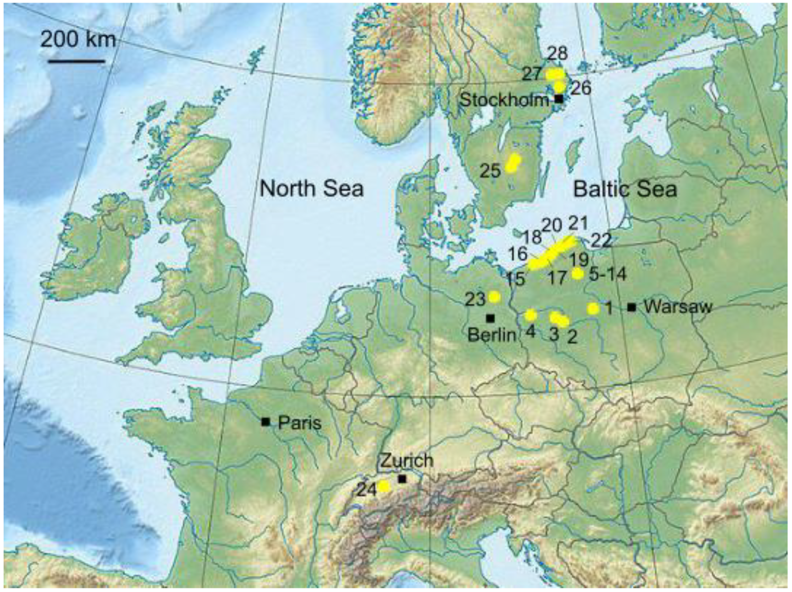
2.1. Data Collection

Hydrochemical data from lakes used in this study involved a series of EC, Ca²⁺, Mg²⁺, K⁺, Na⁺, HCO₃⁻, SO₄²⁻, Cl⁻ and NO₃⁻ monitoring survey data from a number of natural glacial and coastal lakes in Poland, Germany, Switzerland, and Sweden. The lakes covered a salinity range from 0.01 to 5.4 ppt. Details on the location of lakes, data collection, and availability are given in Figure 1 and Table S1.

The procedure of data selection involves a few steps. After checking the completeness of hydrochemical records (i.e., if each chemical species required was determined), the ion charge balance (ICB) was calculated to assess the quality of measurements. After eliminating outliers with an ICB error > 10%, the ratio of total dissolved solids (TDS; mg·L⁻¹) calculated from the ion composition of water (TDS_IC) to the TDS obtained from EC (TDS_EC) was checked. TDS_IC was presumed equal to the sum of the concentration of major ions C_i, which is expressed as follows:

$$TD{S}_{IC} \left[\mathrm{mg}·{\mathrm{L}}^{-1}\right]={\displaystyle \sum }_{i=1}^n{C}_i$$

(2)

The TDS_EC was calculated using the formula (Equation (3) [21]), where

$$TD{S}_{EC} \left[\mathrm{mg}·{\mathrm{L}}^{-1}\right]=0.65·EC$$

(3)

Because the factor of proportionality in Equation (3) varies between 0.55 and 0.90 [21,22,23] and our database involves different hydrochemical types of water (Figure S2), the cut-off range of TDS_IC/TDS_EC was set to −15/+35%. Such a procedure led us to select 864 records to develop model equations.

2.2. Water Analyses

Most water chemical data included in the database were taken from the available published reports; however some records were collected by the authors that had not been published yet (Table S1). In such cases, the ion composition of water was analyzed using a standard methodology. This involved ion chromatography for Cl⁻, SO₄²⁻ and NO₃⁻ (881 Compact IC Pro; Metrohm, Herisau, Switzerland), titration with 0.05 M HCl with regard to methyl orange and phenolphthalein for HCO₃⁻ and CO₃²⁻ (ISO9963 [24] as well as AAS for Ca²⁺, Mg²⁺, K⁺ and Na⁺ (NovAA300; Analytik Jena GmBH, Jena, Germany) [25]. Analytical quality was verified with certified reference materials (Harbour water, NWHAMIL-20.2) and an ion charge balance.

2.3. Chemical Calculations

Ionic strength (I; mol·L⁻¹) was calculated on the basis of molarities m_i and charges z_i of individual ions (Ca²⁺, Mg²⁺, K⁺, Na⁺, HCO₃⁻, SO₄²⁻, Cl⁻ and NO₃⁻) with the formula in Equation (4):

$$I=\frac{1}{2}{\displaystyle \sum }_{i=1}^{i=n}{m}_i·z_i^2$$

(4)

The transport numbers (t_i), approximating the contributions of individual ions in the total conductivity of the mixed electrolyte solution, were assessed on the basis of ionic molar conductivities of the ions (λ_i) and their molalities (M_i; mol·kg⁻¹) using Equations (5) and (6) [20]

$$t_i=\frac{{\lambda }_i·M_i}{\kappa }=\frac{{\lambda }_i·M_i}{{\sum }_{i=1}^n{\lambda }_i·M_i}$$

(5)

where

$${\lambda }_i={\lambda }^{°}\left(T\right)-\frac{A\left(T\right)·I^{1/2}}{1+B·I^{1/2}}$$

(6)

λ°(T), A(T), and B are derived from empirical equations given by McCleskey et al. [20].

CO₂ partial pressures (pCO_2aq; bar) in lake water were determined computationally on the basis of pH and the activity of HCO₃⁻ [26,27,28,29,30,31]. The mathematical expression for this calculation is as follows:

$$pC{O}_2\approx \left[H_{2}C{O}_3\right]=\frac{{10}^{-pH}·\left[HC{O}_3^{-}\right]}{K_1}$$

(7)

where K₁ indicates the temperature-dependent equilibrium constant in H₂CO₃→H⁺ + HCO₃⁻ system and is obtained from the empirical formula reported by Kelts and Hsü [32]. Because Abril et al. [33] showed that the pCO₂ obtained was highly affected by pH, alkalinity, and DOC, calculations were only performed for the samples with circumneutral/alkaline pH and alkalinity > 1000 µmol·L⁻¹, as recommended by Abril et al. [33]. CO₂ saturation was expressed as ΔpCO₂ in relation to pCO₂ in equilibrium with atmospheric CO₂. Positive ΔpCO₂ ΔpCO₂ indicated supersaturation, while negative showed undersaturation (and, thus, the absorption of CO₂ from ambient air).

Activity coefficients γ_i were derived using the Debye–Hückel equation (Equation (8)) and temperature-dependent coefficients A and B, including the ionic radius (r_i) and ion charge (Z_i) from [34]. Thus,

$${\gamma }_i=\frac{-A·Z_i^2·\sqrt{I}}{1+r_i·B·\sqrt{I}}$$

(8)

The saturation index for calcite (SI_calc) was obtained from the activities of Ca²⁺, CO₃²⁻ (values in brackets in Equation (9)) and the calcite solubility coefficient was obtained at in situ temperature K_c.

$$S{I}_{calc}=\frac{\left[C{a}^{2+}\right]\left[C{O}_3^{2-}\right]}{K_c}$$

(9)

The K_c was computed using an empirical equation given by Tchobanoglous et al. [17].

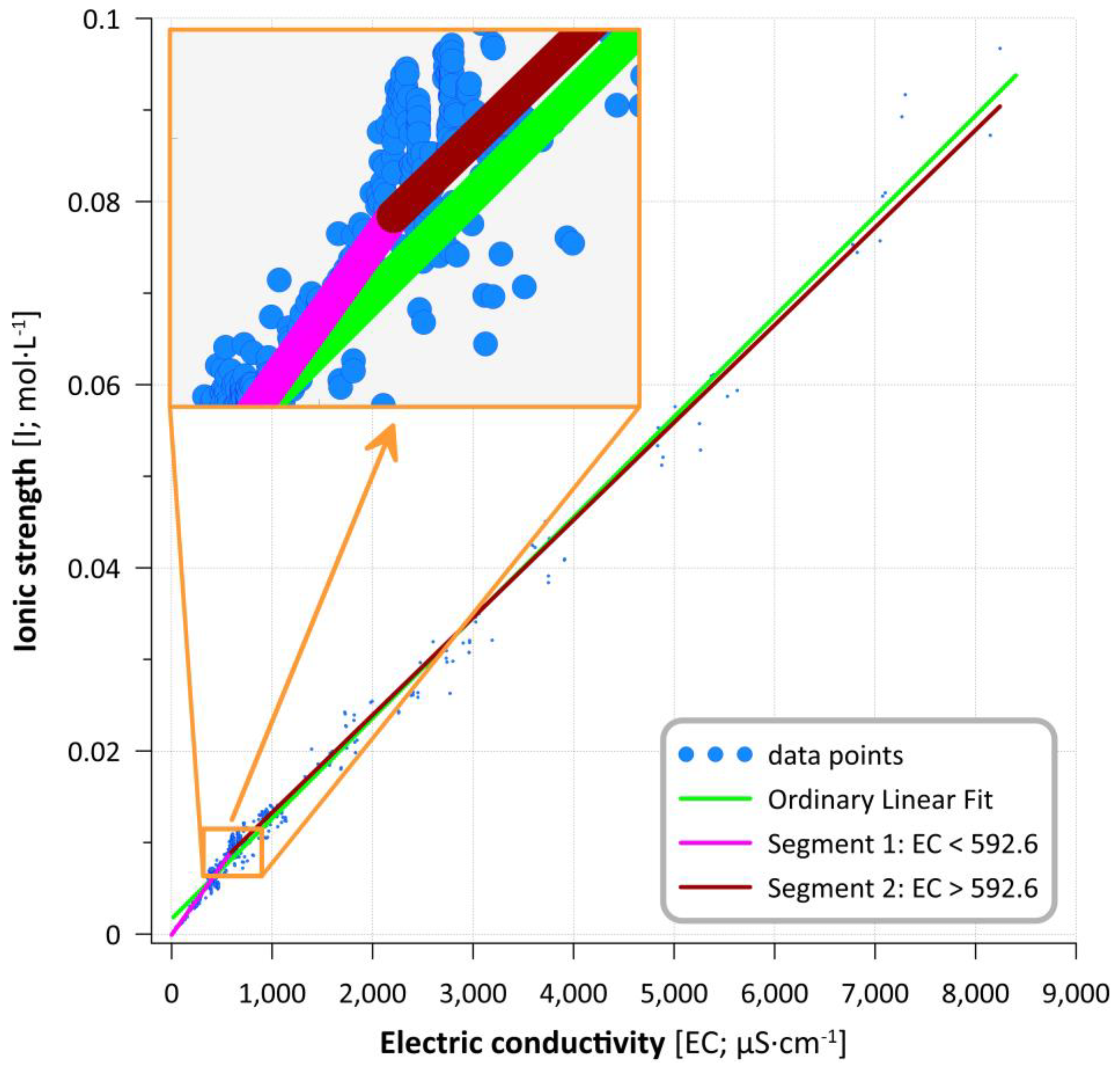
2.4. Model Development

Our preliminary tests showed that the best fitting of the regression model of EC vs. I could be achieved using segmented (and not ordinary linear) regression (also known as piecewise regression or broken-stick regression [35,36]. To determine the optimal number of segments, as well as to assess the reliability and stability of the model developed, the bootstrapping method (i.e., random sampling with replacement) was used. From the initial dataset, 1000 subsamples, encompassing 90% of the records, were randomly selected and processed with the use of the “segmented” R package (ver. 1.6-2; [37,38]). An assessment of the optimal number of segments was performed in two ways. The first approach used the Bayesian information criterion (BIC), and the second used the Davies test [39].

For each of the 1000 subsamples, both ordinary linear regression (i.e., without breakpoint) and two-segment linear regression models were fitted using the least squares method. To compare models, the Akaike information criterion (AIC) and BIC [40,41] were used. These methods were applied to assess the information loss by a given model as they measure a balance between the model quality (i.e., goodness of fit) and simplicity (i.e., the number of parameters involved). In other words, AIC and BIC enable model overfitting and underfitting to be avoided. The formula for the BIC is similar to that for the AIC, albeit a difference exists between them with regard to “penalty” for the number of parameters included. The use of AIC and BIC to create regression models was tested by Yang [42]. From [42], it follows that AIC acts as an asymptotic optimal for selecting a model with the lowest mean squared error whenever the “true model” is not among the models compared. BIC, on the other hand, is highly effective when one of the models tested is the “true model”.

The statistical significance of the segmented model was tested using the Davies test [38,43]. The reason for using this test as an alternative to classical methods was that it provided a better estimation of p values. The p values obtained with classical tests seemed to be 3- to 5-fold underestimated.

From the 1000 segmented regression models developed, the final model describing the relationship between EC and I was calculated as a medoid, i.e., the multidimensional median. The medoid was computed for five parameters, such as the position of the break point, slope, and intercept of the first segment, as well as the slope and intercept of the second segment of the regression models. Prior to calculations, data were standardized, and calculations were performed using the “pam” function of the “cluster” R package [44].

2.5. Model Validation

Model validation was performed on 161 samples obtained from open-source databases such as the Waterbase—Water Quality ICM—European Environment Agency: https://www.eea.europa.eu/data-and-maps/data/waterbase-water-quality-icm-2 (accessed 3 October 2023), Water chemistry (Great Lakes nearshore areas: https://data.ontario.ca/dataset/water-chemistry-great-lakes-nearshore-areas (accesses 3 October 2023), Water Chemistry of lakes in the southwest Florida Water Management District: https://www.swfwmd.state.fl.us/media/938 (accessed 3 October 2023) as well data from Lake Kierskie (Poland) [45]. The data above encompassed EC and the major ion composition of water samples. Based on these data, the ionic strength of the real solution was calculated (empirical I; I_emp). The validation results were expressed as the relative error (ε%; Equation (10)) between the modeled I value (I_mod) and empirical I value (I_emp) obtained from the analytical concentration data (Equation (4)) using the following formula:

$$\epsilon \%=\frac{I_{mod}-I_{emp}}{I_{emp}}·100\%$$

(10)

3. Results and Discussion

3.1. Data Characterization

The lake water sampled in this study displayed a wide spectrum of chemical composition and represented all major categories of water distinguished by Gibbs [8] (Figure S2). The TDS varied in a broad range from 12 to 5375 mg·L⁻¹, translating into an EC of 19 to 8242 μS·cm⁻¹, respectively. Such a TDS range corresponded to limnetic and oligohaline water [21]. However, the frequency distribution of samples in different TDS/EC intervals was highly and positively skewed (Figure S3). The water between 250 and 818 μS·cm⁻¹ was by far the most abundant group encompassing c.a. 67% of the dataset.

On the basis of EC, lake water can be classified as weakly (EC < 250 μS·cm⁻¹), moderately (250 < EC < 750 μS·cm⁻¹), highly (750 < EC < 2250 μS·cm⁻¹) and very highly mineralized (EC > 2250 μS·cm⁻¹) [46]. The first group encompassed Swedish lakes (no. 25–28 in Table S1), the lakes of the Bory Tucholskie area (no. 5–14 in Table S1), as well as Lake Stechlin and Rotsee (no. 23–24 in Table S1). Moderately mineralized lakes were represented by Lake Licheńskie, Lake Łódzko-Dymaczewskie, Lake Dębno, Lake Trześniowskie (no. 1–4 in Table S1), Lake Sarbsko and Rotsee (no. 22 and 24 in Table S1). Highly and very highly mineralized water only occurred in coastal lakes of the Polish Baltic coast (no. 15–21 in Table S1). Weakly mineralized water displayed a similar t_i for different ions, albeit with slightly higher values for Ca²⁺ (

Table 1. Average transport numbers (t_i) for the groups of lakes. The values given show the contributions of particular chemical species into the total electrical conductivity of the solution.

Lake Mineralisation	EC	ti
	μS·cm−1	Na+	Ca2+	Mg2+	K+	HCO3−	SO42−	Cl−	NO3−	Dival. Ions	Monoval. Ions
Weak	<200	0.13	0.25	0.10	0.03	0.14	0.17	0.18	0.01	0.48	0.52
Moderate	200–750	0.07	0.32	0.09	0.01	0.27	0.12	0.11	0.00	0.46	0.54
High	750–2250	0.17	0.16	0.09	0.02	0.12	0.10	0.34	0.00	0.65	0.35
Very high	>2250	0.27	0.04	0.07	0.01	0.03	0.05	0.53	0.00	0.84	0.16

). Comparable contributions from divalent and monovalent ions to the total conductivity indicated that the EC of lake water was due to the combined effect of Ca²⁺, Cl⁻, SO₄²⁻, HCO₃⁻, and Na⁺. Moderately mineralized lake water also displayed similar total t_i values for divalent and monovalent ions, but the EC was primarily due to Ca²⁺ and HCO₃⁻ with a minor role of other species (Table 1). In highly and very highly mineralized water, monovalent ions by far predominated in shaping conductivity. In the former group, the overall t_i of monovalent ions was 0.65 and, in the latter, 0.84 (Table 1). Respective contributions from the divalent ions ranged from 0.35 in highly mineralized lakes to 0.16 in very highly mineralized water. In general, anions were more influential on conductivity than cations, albeit the role of NO₃ was negligible in all lakes studied (Table 1).

3.2. Modeling Results

The identification of the optimal model describing the relationship between EC and I required that the quality of models with n segments (where n ≥ 1) were checked. In the “segmented” R package used in this study, the number of breakpoints, as well as the optimum number of breakpoints, was assessed using BIC. The Davies test, in turn, enabled a comparison between ordinary linear regression and double-/triple-segment models.

Both approaches were applied to 1000 random subsamples. Using BIC, a maximum number of six segments were tested. The minimum BIC value, as well as the Davies test, indicated that the double breakpoint model (i.e., consisting of 3 segments) was optimal for our dataset. However, while the Davies test unambiguously supported the double breakpoint pattern as the best model, the BIC was less consistent. Indeed, the double breakpoint model was also favored in this approach, but three-, four-, and even five-point models were also obtained in several subsamples. In addition, in several other cases, the BIC was inconclusive altogether, and any number of segments could be chosen as an optimal fit. A very important result was that the first breakpoint (BP₁) was concordantly positioned with both methods in a narrow range of EC values around 592 µS·cm⁻¹. From Figure S4, it emerged that in 50% of the subsamples tested, the BP₁ obtained was within an <2 µS·cm⁻¹ interval between 592 and 594 µS·cm⁻¹, and in 80% of the subsamples, values ranged between 590 and 597 µS·cm⁻¹ (i.e., within 7 µS·cm⁻¹-wide interval). The arithmetic mean value of BP₁ from 1000 models was 591.99 µS·cm⁻¹ (Figure S4). However, because the above number was non-existent in the dataset analyzed, BP₁ was set to the nearest “real” value, which was 592.6 µS·cm⁻¹. Given that the precision of EC measurements with digital conductometers is typically around 1% (relative to the mean BP₁ value of 592.6 µS·cm⁻¹, this translates into c.a. 6 µS·cm⁻¹), the dispersion of results is totally within the instrumental error. The reliability of the estimated BP₁ value was further corroborated by the similarity between the mean BP₁ of 591.99 µS·cm⁻¹ as well as the median BP₁ (593.0 µS·cm⁻¹) and modal BP₁ values (593.3 µS·cm⁻¹). On the other hand, the second breakpoint, BP₂, was more difficult to find. BIC put it at 4000–4500 µS·cm⁻¹ while, from the Davies test, it emerged that the BP₂ was at 600, 1000–1500 and 2500–3000 µS·cm⁻¹. This variability could, in large part, be related to the fact that the distribution of the EC values in the dataset was highly skewed, with EC > 4000 µS·cm⁻¹ being rather underrepresented. This fact could have affected the model’s stability. Considering the differences in the positioning of the BP₂, a decision was made that the double-segment regression model (i.e., with one breakpoint) was the most appropriate for the dataset analyzed.

Having chosen the double-segment model as the most suitable to explain the EC vs. I relationship, its robustness was verified using an array of statistical tests. First, when the AIC and BIC values for ordinary linear regression and double-segment regression were compared (Figure S5), it became clear that the latter model was more advantageous than the former. The increase in the number of parameters used in the model from 2 (for the slope and intercept) for ordinary regression to 4 (2 values for slope and 2 values for the intercept in segmented regression) was compensated by a reduction in the model error (residuals) values. It is underlined that the differences between AIC and BIC values for ordinary and segmented regression models were significantly higher than their distance from the line of equality between both models (1:1 line in Figure S5). This corroborated that, despite the appreciable variability in the quality of the models developed, the segmented regression model was always better fitted to empirical data than ordinary linear regression. Second, for each segmented regression model developed, the Davies tests were calculated [38,43] to verify the statistical significance of the differences between slopes for the model segments. The results clearly show that the slopes were significantly different. The probability (p values) that these differences were only due to chance was exceedingly low and varied from 1.90⁻¹⁰⁶ to 1.65⁻⁵⁵, with 4.49⁻⁵⁸ on average. The distribution of p values was highly positively skewed (Sk = 22.82) and leptokurtic (kurtosis = 595.14). The median of the probability distribution Me = 8.98⁻⁶³ was considerably lower than the average.

We also found that the slopes and intercepts of the model segments showed inversely proportional relationships, i.e., the increase in the slope/intercept of the first segment (encompassing the lowest EC values) was accompanied by a decrease in the slope/intercept of the second segment. However, these relationships were rather weak and non-linear. In each of the 1000 random subsamples, the slope of the first segment was always higher than the slope of the second segment. On the other hand, the intercept of the first segment was always lower than that of the second segment.

The final version of the relationship between EC and I emerging from our modeling approach consisted of two linear segments with a breakpoint at 592.6 µS·cm⁻¹. The equations are parametrized as follows:

I_mod = 15.231 × 10⁻⁶·EC − 79.191 × 10⁻⁶ for EC < 592.6 µS·cm⁻¹

(11)

and

I_mod = 10.647 × 10⁻⁶·EC + 26.373 × 10⁻⁴ for EC > 592.6 µS·cm⁻¹

(12)

The fit of this model to empirical data is shown in Figure 2.

Deviations between the I predicted with ordinary linear regression and the values obtained using the segmented model in relation to the average I in the empirical dataset (0.0099 mmol·L⁻¹) were different between −8.0 and +16.0%. The mean relative difference between the models was +4.35% (with a standard deviation of 7.13), which indicated that, in relation to segmented regression, the ordinary linear regression tended to overestimate the values of I. The highest positive deviations (>+4%) were for EC < 312 µS·cm⁻¹ as well as for EC > 4500 µS·cm⁻¹. The highest negative deviations (<−4%) occurred for EC between 500 and 1832 µS·cm⁻¹.

The stepwise relationship between EC and I depicted by Equations (11) and (12) makes the model substantially different from hitherto used empirical and ordinary linear relationships [14,17,19]. As far as we are concerned, segmented regression is better suited to empirical data not only for statistical reasons but also because it more reliably mirrors the influence of the major ion composition on the ionic strength and the conductivity of natural waters. From Equation (4), it follows that polyvalent ions affect ionic strength more strongly than monovalent ions because the I value is proportional to the square of the ion charge. At the same time, as shown by [20], the conductivity is to a large degree controlled by the valency of dissolved chemical species and, for example, for a 0.1 mol·L⁻¹ HCO₃⁻ solution, the EC is around 3870 μS·cm⁻¹, while the EC of the Ca²⁺ solution of the same molarity is ca. 8300 μS·cm⁻¹. Consequently, the changes in EC vs. I due to the increase in concentrations of monovalent ions follow a less steep trend than for divalent ions (Figure 3).

From the Gibbs diagram (Figure S2), it emerges that the chemical composition of lake water varies greatly along the salinity (and conductivity) gradient. Highly mineralized water (>750 μS·cm⁻¹) in our dataset was enriched in monovalent ions (Na⁺ and Cl⁻ in particular) compared to weakly and moderately mineralized water, and consequently, these ions were the primary carriers of conductivity. The contributions of monovalent ions to the total EC of highly mineralized water were 0.65–0.84 (Table 1). On the contrary, at EC < 750 μS·cm⁻¹, the transport numbers for divalent ions, t_i, were 0.52–0.54 (Table 1), thus indicating that divalent ions (Ca²⁺ in particular) were more influential in shaping conductivity. Given the critical role that the ion composition had for EC and I of the solutions, it seems reasonable to conclude that a chemical change from Ca²⁺-dominated to Na⁺/Cl⁻ dominated water accompanying an increase in salinity translated into the flattened EC vs. I trend at high conductivity values.

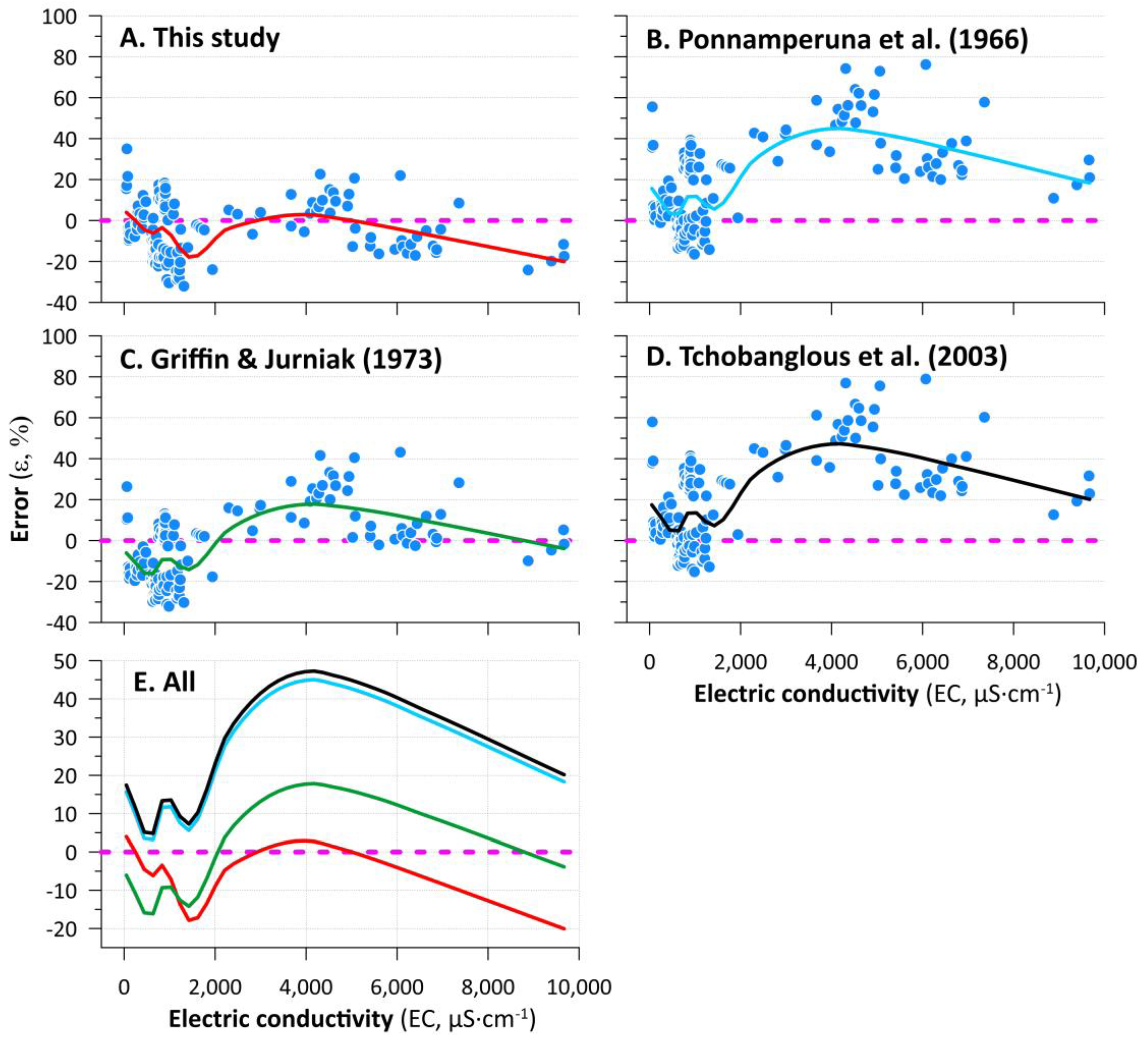
3.3. Model Validation

The mean relative error of I estimation with Equations (11) and (12), ε%, for the total conductivity range was −3.4%; however, these values showed some variability with EC (Figure 4A;

Table 2. Relative error of estimation for I on the basis of EC (ε%) with different empirical formulae. The lowest values indicating the best prediction are marked in bold. The model equations developed in this study provide better perditions throughout most of the conductivity range investigated.

Conductivity [μS·cm−1]	This Study	Ponnamperuna [18] #	Griffin and Jurniak [13] &	Tchobanoglous et al. [16] *
<250	1.1	13.1	−8.1	14.8
250–500	2.1	8.9	−11.5	10.7
500–1000	−3.5	11.0	−9.8	12.7
1000–2500	−12.6	11.3	−9.6	13.0
2500–5000	6.6	51.1	22.7	53.4
5000–7500	−6.9	34.5	9.3	36.6
>7500	−17.8	20.4	−2.2	22.3

Notes: ^# I = 0.016·EC [mmho]; ^& I = 0.013·EC [mmho]; * I = 2.5 × 10⁻⁵·TDS [mg·L⁻¹].

). The lowest ε% was for EC < 1000 μS·cm⁻¹ (encompassing most freshwater lakes) as well as for 2500–7500 μS·cm⁻¹ and, for these conductivity ranges, our model gave much better adjustment to the data than other models (Figure 4A–E). On the other hand, the model seems to underpredict the I for EC between 1000 and 2500 μS·cm⁻¹ and for >7500 μS·cm⁻¹. Slightly better results for these ECs were obtained using the equation shown in [13].

3.4. Potential Implications of the Model

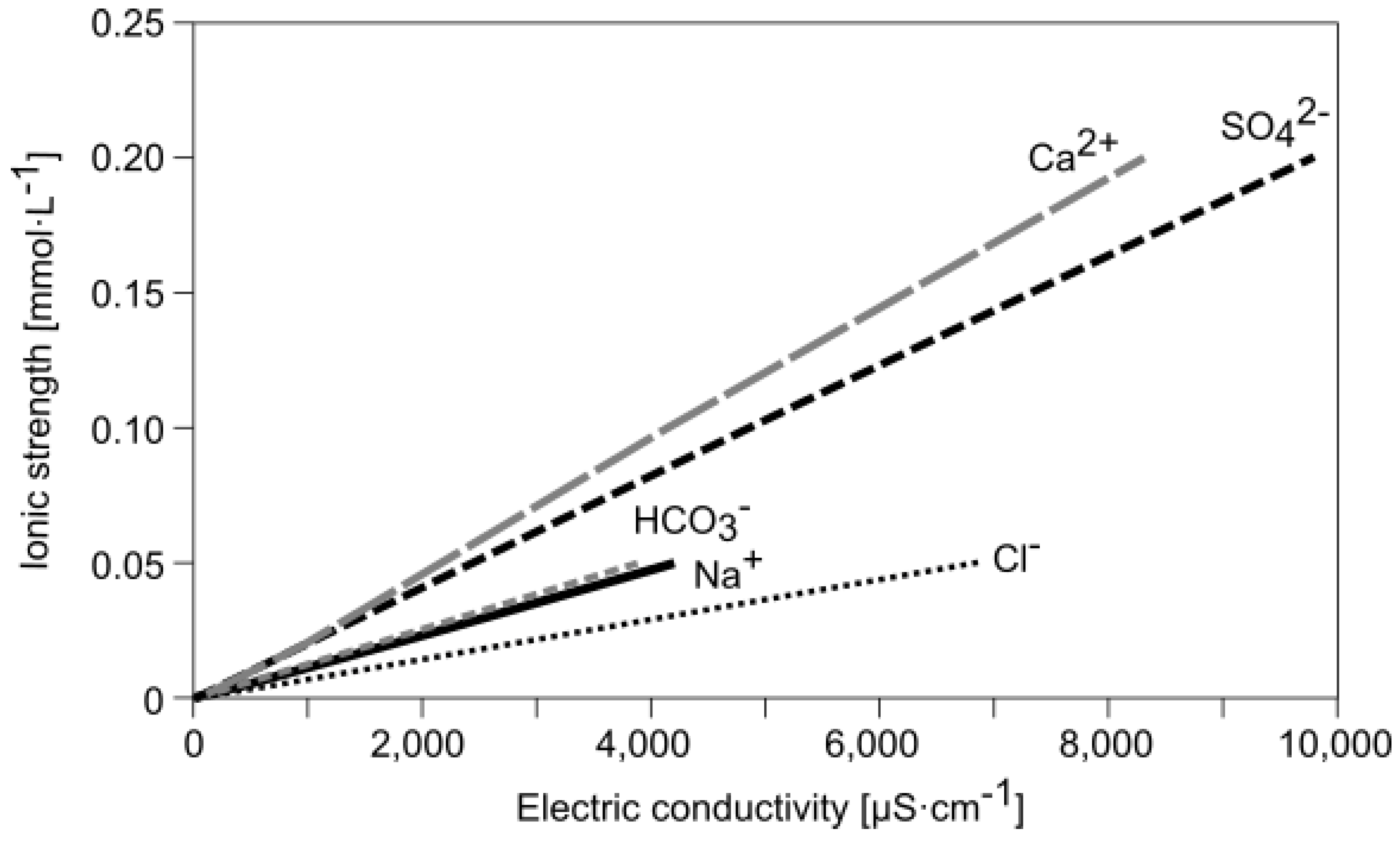
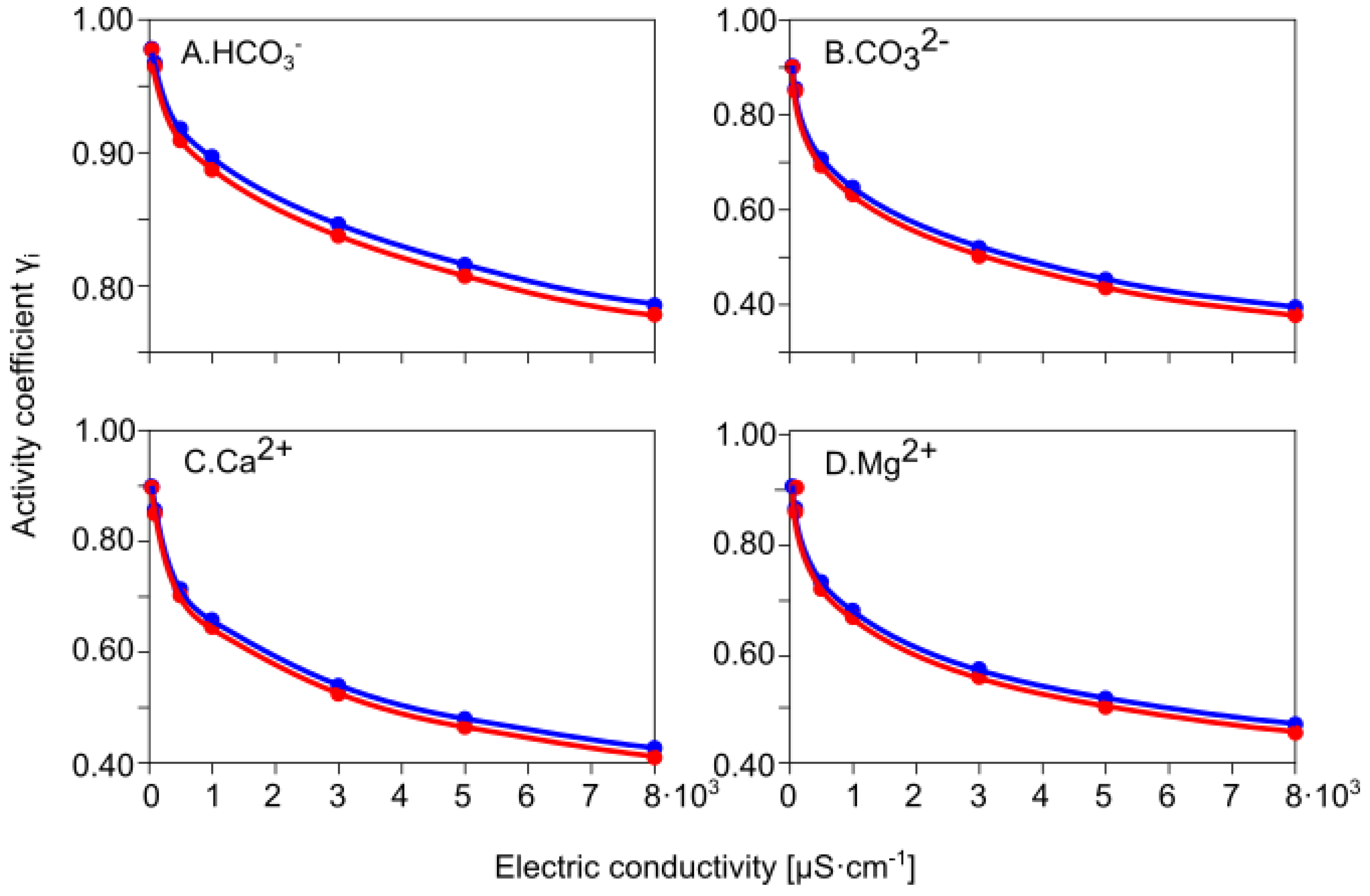
3.4.1. Calculating γ Activity Coefficients for Major Ions

Activity coefficients are indispensable for obtaining effective concentrations of ions in solutions and, thus, are of vital importance for chemical calculations and the modeling of chemical processes in natural water. Despite the fact that there are at least a few approaches to calculate γ, in each of them, ionic strength acts as a key variable. Using our model, we calculated γ activity coefficients for four ions occurring in high concentrations in temperate lakes (Ca²⁺, Mg²⁺, HCO₃⁻, CO₃²⁻), for temperatures between 0 and 30 °C and EC ranging from 50 to 8000 μS·cm⁻¹. The results of these calculations are shown in Figure 5 and Tables S2–S5.

For all ions, the γ coefficients decreased with increasing EC and temperature, albeit the fact that the effect of temperature seemed to be very weak, especially at low conductivities. This fact agrees with a theory, and for this reason, for the sake of simplicity, temperature is sometimes eliminated from the expressions for γ [17]. The strongest temperature influence on γ was obtained for CO₃²⁻ and showed an up to 4.1% decrease in γ, respectively, at 30 °C. This species also showed the highest differences in γ over the EC range considered. The values of the γ coefficient for CO₃²⁻ dropped from around 0.90 at 50 μS·cm⁻¹ to 0.36–0.39 at 8000 μS·cm⁻¹. Divalent cations (Ca²⁺, Mg²⁺) also demonstrated a considerable decrease in activity resulting from enhanced I; however, the γ at a maximum EC was slightly higher than for CO₃²⁻ and ranged from 0.41 to 0.45. On the other hand, the activities of HCO₃⁻ were much less affected by ionic strength. Over our EC range, the activities of bicarbonates declined from 0.97 to 0.76–0.78.

3.4.2. Calculating Carbonate Saturation of Lake Water

As far as we are concerned, the γ_i values given in Tables S2–S5 can be applied to hydrological/limnological monitoring. Below, we used these values to calculate SI_calc in lake water based on data from Lake Kierskie, Poland [45]. The calculations were run using different approaches: (i) for the full ion composition of lake water which allowed the true SI_calc values to be approximated, hereafter referred to as SI_full, (ii) using the Langelier SI (LSI) calculator available at: https://www.lenntech.com/ro/index/langelier-explanation.htm (accessed on 3 October 2023) (and applied by [45]) and (iii) using the γ coefficients for HCO₃⁻ and Ca²⁺ from Tables S2 and S4, respectively, to obtain modeled SI_calc (SI_model). The idea behind these calculations was to check the recovery of SI_full with different calculation methods.

From the results (Figure S6), it emerged that the SI_calc estimations based on modeled γ values (SI_model) better reproduced the SI_full than the LSI. The regression equation for the SI_full–SI_model relationship indicates that SI_model values systematically underestimated the SI_full by c.a. 0.01 (0.01–0.02), while the LSI values were c.a. 0.25 (0.22–0.26) lower than the SI_full.

3.4.3. Screening of Spatial Distribution of pCO₂ in Lakes

In the summers of 2018, 2019, and 2020, we sampled 64 lakes across the Masurian and Suwałki Lake Districts, Poland (Figure S7). In each lake, we measured physical–chemical parameters (temperature, EC, pH) and HCO₃⁻ concentrations on the surface water layer. The model developed allowed the screening of one of the largest lakelands in Poland for the distribution of the pCO₂ values and potential tendencies for the absorption/emission of CO₂ from/to the atmosphere. One lake was excluded from the calculations (Lake Tyrsko) because of its too-low alkalinity (860 µmol·L⁻¹). From the calculations, it emerged that pCO₂ ranged from 0.09 to 7.05 mbar, translating into 3.28–247 μmol CO₂·L⁻¹. In 20 lakes, the pCO₂ obtained was slightly lower than the equilibrium of CO₂ concentrations in lake water of approximately 14.171 μmol·L⁻¹ [48] (ΔpCO₂ from −11 to −0.2 μmol·L⁻¹ below equilibrium), arguing for their autotrophic character. The autotrophic lakes (i.e., absorbing CO₂ from the atmosphere) were primarily located in the Suwałki Lake District. On the other hand, positive ΔpCO₂, indicative of heterotrophy (i.e., emission of CO₂ from the ambient atmosphere), occurred in most lakes studied, though it varied in a broad range from 233 to 0.1 μmol·L⁻¹.

3.4.4. Temporal Changes in pCO₂ in Lakes

Our method can also be used to trace temporal changes in pCO₂ in lakes at different timescales and seems to be particularly advantageous when using historical data to obtain information on long-term CO₂ trends where there is no possibility to measure CO₂ directly. Clearly, calculations can only be made for water that has a circumneutral and alkaline pH and alkalinity above 1000 µmol·L⁻¹, as recommended by [33]. To illustrate this based on t, pH, EC and HCO₃⁻ values for lake surface water, we have calculated pCO₂ for a group of five lakes near Konin (encompassing Lake Gosławskie, Lake Licheńskie, Lake Ślesińskie and Lake Wąsosko-Mikorzyńskie, here referred to as Konin lakes), which since the 1960s, has received heated water from nearby power plants and has thus become thermally polluted [49]. The calculations showed that between 2015 and 2021, the pCO₂ values in these lakes ranged between 0.23 and 6.91 mbar and there were no statistically significant differences between the lakes (Figure S8). However, the pCO₂ varied greatly throughout each year with maximum values in winter and minimum during the spring and summer. The pCO₂ in Konin lakes implies that for the most part of the period studied, lakes were heterotrophic (ΔpCO₂ > 0). Autotrophy occurred only sporadically during spring and summer (Figure S8).

Similar calculations were performed for Lake Suminko (Kashubian Lake District, Poland) and Lake Kierskie (Poznań Lake District, Poland) (Figure S9). For the former, we used monitoring data collected between October 2007 and May 2010 by Tylmann et al. [50], while the latter was monitored between November 2015 and October 2016 by Apolinarska et al. [45]. The pCO₂ in Lake Suminko and Lake Kierskie varied between 0.19 and 14.3 mbar and from 0.22 to 10.5 mbar, respectively (Figure S9A,B) and thus were slightly higher than in Konin lakes, but displayed similar annual pattern. Lake Suminko displayed a relatively long period of autotrophy between April and September 2009 as well as in April/May 2010 (Figure S9A), while Lake Kierskie was autotrophic between June and September 2016 (Figure S9B). For Lake Kierskie, we had the possibility to compare the modeled pCO₂ with the values calculated on the basis of the full chemical composition of lake water samples. The relative error ε% obtained was between −0.24 and −0.95%.

3.4.5. Spatial CO₂ Distribution in Lakes

The monitoring of greenhouse gas (GHG) emissions from lakes requires the careful selection of representative sites in which long-term observations can be collected. Provided that the distribution of CO₂ in lake water is often highly irregular [51,52], the selection of site(s) (or a number of sites) should be preceded by a screening of the lake studied to recognize the variability of the gas and its distribution. Our method allows for the relatively rapid collection of data on CO₂ distribution throughout a water body. For the sake of demonstration between March 2022 and February 2023, with the monthly resolution, we collected hydrochemical data from three stations across Lake Licheńskie, and one of the thermally polluted Konin lakes [49]. To check the effect of the input of heated, water on CO₂ productivity in Lake Licheńskie, we took water samples in front of the mouth of the canal, delivering cooling effluents to the lake as well as in two thermally different parts of the lake (Figure S10). From our results, it emerged that the sites studied indeed showed differences in pCO₂ values from 0.2 to 1.9 mbar in the least heated section to 0.6–5.5 mbar at the inflow of PPK water to the lake (Figure S10); however, contrary to what was expected, on a yearly basis, these differences were not statistically significant. Despite the fact that the lake is net heterotrophic, some parts of the lake may temporarily show autotrophy (e.g., site L3 in Figure S10).

4. Conclusions

The paper outlines the empirical model for calculating the ionic strength (I) of natural waters from electric conductivity. The model consists of two simple linear equations for different EC ranges and is applicable for oligohaline and freshwater lacustrine systems; however, the best results were obtained for EC < 1000 µS·cm⁻¹. The performance of the model at EC > 1000 µS·cm⁻¹ could be improved by collecting more hydrochemical data from oligohaline water. The method allows for a rapid determination of a number of standard hydrochemical parameters such as ion activity coefficients, pCO₂, and saturation states for different minerals. This method is dedicated to limnological and hydrobiological applications and can be used for the standard monitoring of biogeochemical processes in the lake water column. It should be underlined, however, that the approach proposed should only be used when data on the full ion composition of water samples is unavailable, especially for pCO₂ calculations.

References

1. Woolway, R.I.; Benjamin, M.; Kraemer, B.M.; Lenters, J.D.; Merchant, C.J.; O’Reilly, C.M.; Sharma, S. Global lake responses to climate change. Nat. Rev. 2020, 1, 388–403. [Google Scholar] [CrossRef]
2. Bartosiewcz, M.; Przytulska, A.; Lapierre, J.F.; Laurion, I.; Lehmann, M.F.; Maranger, R. Hot tops, cold bottoms: Synergistic climate warming and shielding effects increase carbon burial in lakes. Limnol. Oceanogr. Lett. 2019, 4, 132–144. [Google Scholar] [CrossRef]
3. Cheng, J.; Xu, L.; Jiang, M.; Jiang, J.; Xu, Y. Warming Increases Nitrous Oxide Emission from the Littoral Zone of Lake Poyang, China. Sustainability 2020, 12, 5674. [Google Scholar] [CrossRef]
4. Guo, M.; Zhuang, Q.; Tan, Z.; Shurpali, N.; Juutinen, S.; Kortelainen, P.; Martikainen, P.J. Rising methane emissions from boreal lakes due to increasing ice-free days. Environ. Res. Lett. 2020, 15, 064008. [Google Scholar] [CrossRef]
5. Hofmann, H. Spatiotemporal distribution patterns of dissolved methane in lakes: How accurate are the current estimations of the diffusive flux path? Geophys. Res. Lett. 2013, 40, 2779–2784. [Google Scholar] [CrossRef]
6. del Sontro, S.; Beaulieu, J.J.; Downing, J.A. Greenhouse gas emissions from lakes and impoundments: Upscaling in the face of global change. Limnol. Oceanogr. 2018, 3, 64–75. [Google Scholar] [CrossRef] [PubMed]
7. Gibbs, R.J. Mechanisms controlling world water chemistry. Science 1970, 170, 1088–1090. [Google Scholar] [CrossRef]
8. Wu, T.; Zhu, G.; Zhu, M.; Xu, H.; Zhang, Y.; Qin, B. Use of conductivity to indicate long-term changes in pollution processes in Lake Taihu, a large shallow lake. Environ. Sci. Poll. Res. 2020, 27, 21376–21385. [Google Scholar] [CrossRef]
9. Groleau, A.; Sarazin, G.; Vinçon-Leite, B.; Tassin, B.; Quiblier-Llobéras, C. Tracing calcite precipitation with specific conductance in a hard water Alpine lake (Lake Bourget). Water Res. 2000, 34, 4151–4160. [Google Scholar] [CrossRef]
10. Escoffier, N.; Perolo, P.; Many, G.; Tofield Pasche, N.; Perga, M.-E. Fine-scale dynamics of calcite precipitation in a large hardwater lake. Sci. Total Environ. 2023, 864, 160699. [Google Scholar] [CrossRef]
11. Kester, D.R.; Pytkowicz, R.M. Magnesium sulfate association at 25 °C in synthetic seawater. Limnol. Oceanogr. 1968, 13, 670–674. [Google Scholar] [CrossRef]
12. Stumm, W.; Morgan, J.J. Aquatic Chemistry, Chemical Equilibria and Rates in Natural Waters, 2nd ed.; John Wiley & Sons, Inc.: New York, NY, USA, 1981; 780p. [Google Scholar]
13. Griffin, R.A.; Jurniak, J.J. Estimation of activity coefficients from the electrical conductivity of natural aquatic system and soil extracts. Soil Sci. 1973, 116, 26–30. [Google Scholar] [CrossRef]
14. Polemio, M.; Bufo, S.; Paoletti, S. Evaluation of ionic strength and salinity of groundwaters: Effect of the ionic composition. Geochim. Cosmochim. Acta 1980, 44, 809–814. [Google Scholar] [CrossRef]
15. Simón, M.; García, I. Physico-chemical properties of the soil-saturation extracts: Estimation from electrical conductivity. Geoderma 1999, 90, 99–109. [Google Scholar] [CrossRef]
16. Tchobanoglous, G.; Burton, F.L.; Stensel, H.D. Wastewater Engineering Treatment and Reuse, 4th ed.; McGraw-Hill Education: Boston, MA, USA, 2003; 920p. [Google Scholar]
17. McCleskey, R.B.; Nordstrom, D.K.; Ryan, J.N.; Ball, J.W. A new method of calculating electrical conductivity with applications to natural waters. Geochim. Cosmochim. Acta 2012, 77, 369–382. [Google Scholar] [CrossRef]
18. Ponnamperuna, P.N.; Tianco, E.M.; Loy, T.A. Ionic strength of the solutions of flooded soils and other natural aqueous solutions from specific conductance. Soil Sci. 1966, 102, 408–413. [Google Scholar] [CrossRef]
19. Lind, C.J. Specific conductance as a means of estimating ionic strength. U.S. Geol. Survey Prof. Papers 1970, 700-D, D272–D280. [Google Scholar]
20. Anonymous, J. Symposium on the Classification of Brackish Waters. Venice, 8–14 April 1958. The Venice System for the classification of marine waters according to salinity. Limnol. Oceanogr. 1958, 3, 346–347. [Google Scholar] [CrossRef]
21. Pawlowicz, R. Calculating the conductivity of natural waters. Limnol. Oceanogr. Methods 2008, 6, 489–501. [Google Scholar] [CrossRef]
22. McNeil, V.H.; Cox, M.E. Relationship between conductivity and analysed composition in a large set of natural surface-water samples, Queensland, Australia. Environ. Geol. 2000, 39, 1325–1333. [Google Scholar] [CrossRef]
23. Marandi, A.; Polikarpus, M.; Jõeleht, A. A new approach for describing the relationship between electrical conductivity and major anion concentration in natural waters. Appl. Geochem. 2013, 38, 103–109. [Google Scholar] [CrossRef]
24. ISO9963-1:2001; Jakość Wody—Oznaczanie Zasadowości—Część 1: Oznaczanie Zasadowości Ogólnej i Zasadowości Wobec Fenoloftaleiny. 23 April 2001; 10p. Available online: https://sklep.pkn.pl/pn-en-iso-9963-1-2001p.html (accessed on 1 October 2023).
25. Bentley, E.M.; Lee, G.F. Determination of calcium in natural water by atomic absorption spectrophotometry. Environ. Sci. Technol. 1967, 1, 721–724. [Google Scholar] [CrossRef] [PubMed]
26. Borges, A.V.; Delille, B.; Schiettecatte, L.-S.; Gazeau, F.; Abril, G.; Frankignoulle, M. Gas transfer velocities of CO2 in three European estuaries (Randers Fjord, Scheldt, and Thames). Limnol. Oceanogr. 2004, 49, 1630–1641. [Google Scholar] [CrossRef]
27. Cole, J.J.; Prairie, Y.T. Dissolved CO2. In Encyclopedia of Inland Waters; Likens, G.E., Ed.; Elsevier: Oxford, UK, 2009; Volume 2, pp. 30–34. [Google Scholar]
28. Balmer, M.; Downing, J. Carbon dioxide concentrations in eutrophic lakes: Undersaturation implies atmospheric uptake. Inland Waters 2011, 1, 125–132. [Google Scholar] [CrossRef]
29. Henley, S.F.; Annett, A.L.; Ganeshram, R.S.; Carson, D.S.; Weston, K.; Crosta, X.; Tait, A.; Dougans, J.; Fallick, A.E.; Clarke, A. Factors influencing the stable carbon isotopic composition of suspended and sinking organic matter in the coastal Antarctic sea ice environment. Biogeosciences 2012, 9, 1137–1157. [Google Scholar] [CrossRef]
30. Raymond, P.A.; Hartmann, J.; Lauerwald, R.; Sobek, S.; McDonald, C.; Hoover, M.; Butman, D.; Striegl, R.; Mayorga, E.; Humborg Ch Kortelainen, P.; et al. Global carbon dioxide emissions from inland waters. Nature 2013, 503, 355–359. [Google Scholar] [CrossRef] [PubMed]
31. Hastie, A.; Lauerwald, R.; Weyhenmeyer, G.; Sobek, S.; Verpoorter, C.; Regnier, P. CO2 evasion from boreal lakes: Revised estimate, drivers of spatial variability, and future projections. Glob. Change Biol. 2018, 24, 711–728. [Google Scholar] [CrossRef] [PubMed]
32. Kelts, K.; Hsü, K.J. Freshwater carbonate sedimentation. In Lakes Chemistry Geology Physics; Lerman, A., Ed.; Springer: New York, NY, USA, 1978; pp. 295–323. [Google Scholar]
33. Abril, G.; Bouillon, S.; Darchambeau, F.; Teodoru, C.R.; Marwick, T.R.; Tamooh, F.; Ochieng Omengo, F.; Geeraert, N.; Deirmendjian, L.; Polsenaere, P.; et al. Large overestimation of pCO2 calculated from pH and alkalinity in acidic, organic-rich freshwaters. Biogeosciences 2015, 12, 67–78. [Google Scholar] [CrossRef]
34. Berner, R.A. Principles of Chemical Sedimentology; McGraw-Hill: New York, NY, USA, 1971; 240p. [Google Scholar]
35. Seber, G.A.F.; Wild, C.J. Nonlinear Regression; John Wiley & Sons, Inc.: Hoboken, NJ, USA, 1989. [Google Scholar]
36. Muggeo, V.M.R. Estimating regression models with unknown break-points. Stat. Med. 2003, 22, 3055–3071. [Google Scholar] [CrossRef]
37. Muggeo, V.M.R. Segmented: An R package to fit regression models with broken-line relationships. R News 2008, 8, 20–25. [Google Scholar]
38. Muggeo, V.M.R. Package ‘Segmented’. 2022. Available online: https://pypi.org/project/segmented/ (accessed on 1 October 2023).
39. Muggeo, V.M.R. Selecting Number of Breakpoints in Segmented Regression: Implementation in the R Package Segmented. 2020. Available online: https://www.researchgate.net/publication/343737604_Selecting_number_of_breakpoints_in_segmented_regression_implementation_in_the_R_package_segmented (accessed on 1 October 2023).
40. Vrieze, S.I. Model selection and psychological theory: A discussion of the differences between the Akaike information criterion (AIC) and the Bayesian information criterion (BIC). Psychol. Methods 2012, 17, 228–243. [Google Scholar] [CrossRef] [PubMed]
41. Aho, K.; Derryberry, D.W.; Peterson, T. Model selection for ecologists: The worldviews of AIC and BIC. Ecology 2014, 95, 631–636. [Google Scholar] [CrossRef] [PubMed]
42. Yang, Y. Can the strengths of AIC and BIC be shared? A conflict between model identification and regression estimation. Biometrika 2005, 92, 937–950. Available online: https://www.jstor.org/stable/20441246 (accessed on 1 October 2023). [CrossRef]
43. Davies, R.B. Hypothesis testing when a nuisance parameter is present only under the alternatives. Biometrika 1987, 74, 33–43. [Google Scholar] [CrossRef]
44. Maechler, M.; Rousseeuw, P.; Struyf, A.; Hubert, M.; Hornik, K. Cluster: Cluster Analysis Basics and Extensions, R package version 2.1.4. 2022.
45. Apolinarska, K.; Pleskot, K.; Pełechata, A.; Migdałek, M.; Siepak, M.; Pełechaty, M. The recent deposition of laminated sediments in highly eutrophic Lake Kierskie, western Poland: 1 year pilot study of limnological monitoring and sediment traps. J. Paleolimnol. 2020, 63, 283–304. [Google Scholar] [CrossRef]
46. Kemp, A. Organic carbon and nitrogen in the surface sediments of Lakes Ontario, Erie and Huron. J. Sediment. Res. 1971, 41, 537–548. [Google Scholar] [CrossRef]
47. Cleveland, W.S. Robust Locally Weighted Regression and Smoothing Scatterplots. J. Am. Stat. Assoc. 1979, 74, 829–836. [Google Scholar] [CrossRef]
48. Woszczyk, M.; Schubert, C.J. Greenhouse gas emissions from Baltic coastal lakes. Sci. Total Environ. 2021, 755, 143500. [Google Scholar] [CrossRef]
49. Stawecki, K.; Zdanowski, B.; Pyka, J.P. Long-term changes in post-cooling water loads from power plants and thermal and oxygen conditions in stratified lakes. Arch. Pol. Fish. 2013, 21, 331–342. [Google Scholar]
50. Tylmann, W.; Szpakowska, K.; Ohlendorf, C.; Woszczyk, M.; Zolitschka, B. Conditions for deposition of annually laminated sediments in small meromictic lakes: A case study of Lake Suminko (northern Poland). J. Paleolimnol. 2012, 47, 55–70. [Google Scholar] [CrossRef]
51. Schilder, J.; Bastviken, D.; van Hardenbroek, M.; Kankaala, P.; Rinta, P.; Stötter, P.; Heiri, O. Spatial heterogeneity and lake morphology affect diffusive greenhouse gas emission estimates of lakes. Geophys. Res. Lett. 2013, 40, 5752–5756. [Google Scholar] [CrossRef]
52. Loken, L.C.; Crawford, J.C.; Schramm, P.J.; Stadler, P.; Desai, A.R.; Stanley, E.H. Large spatial and temporal variability of carbon ioxide and methane in a eutrophic lake. J. Geophys. Res. Biogeosci. 2019, 124, 2248–2266. [Google Scholar] [CrossRef]
53. Dragon, K.; Górski, J. Identification of groundwater chemistry origins in a regional aquifer system (Wielkopolska region, Poland). Environ. Earth Sci. 2015, 73, 153–2167. [Google Scholar] [CrossRef]
54. Kasperczyk, L.; Modelska, M.; Staśko, S. Pollution indicators in groundwater of two agricultural catchments in Lower Silesia (Poland). Geosci. Rec. 2016, 3, 18–29. [Google Scholar] [CrossRef]
55. Michalska, G. Zróżnicowanie właściwości fizykochemicznych wód podziemnych w zlewni Chwalimskiego Potoku (górna Parsęta, Pomorze Zachodnie. In Funkcjonowanie i Monitoring Geoekosystemów z Uwzględnieniem Zanieczyszczeń Powietrza; Jóźwiak, M., Kowalkowski, A., Eds.; Biblioteka Monitoringu Środowiska: Kielce, Poland, 2001; pp. 305–320. [Google Scholar]
56. Motyka, J.; Gradziński, M.; Różkowski, K.; Górny, A. Chemistry of cave water in Smocza Jama, city of Kraków, Poland. Ann. Soc. Geol. Pol. 2005, 75, 189–198. [Google Scholar]
57. Sojka, M.; Choiński, A.; Ptak, M.; Siepak, M. The Variability of lake water chemistry in the Bory Tucholskie National Park (Northern Poland). Water 2020, 12, 394. [Google Scholar] [CrossRef]
58. Fölster, J.; Johnson, R.K.; Futter, M.N.; Wilander, A. The Swedish monitoring of surface waters: 50 Years of adaptive monitoring. Ambio 2014, 43, 3–18. [Google Scholar] [CrossRef] [PubMed]
59. Gíslason, S.R.; Snorrason, Á.; Ingvarsson, G.B.; Sigfússon, B.; Eiríksdóttir, E.S.; Elefsen, S.Ó.; Hardardóttir, J.; Þorláksdóttir, S.B.; Torssander, P. Chemical Composition, Discharge and Suspended Matter of Rivers in North-Western Iceland; The Database of the Science Institute, University of Iceland: Reykjavik, Iceland; Hydrological Service of the National Energy Authority: Reykjavik, Iceland, 2006; RH-07-2006; 51p. [Google Scholar]
60. Maciejewska, E.; Chmiel, S.; Furtak, T. Zróżnicowanie składu chemicznego wód rzecznych i podziemnych w Roztoczańskim Parku Narodowym. In Wody na Obszarach Chronionych; Partyka, J., Pociask-Karteczka, J., Eds.; Instytut Geografii i Gospodarki Przestrzennej UJ, Ojcowski Park Narodowy, Komisja Hydrologiczna PTG: Kraków, Poland, 2008; pp. 221–227. [Google Scholar]
61. Małek, S.; Gawęda, T. Charakterystyka chemiczna wód powierzchniowych zlewni Potok Dupniański w Beskidzie Śląskim. Sylwan 2005, 2, 29–36. [Google Scholar]
62. Żelazny, M. Czasowo-Przestrzenna Zmienność cech Fizykochemicznych wód Tatrzańskiego Parku Narodowego; Instytut Geografii i Gospodarki Przestrzennej Uniwersytetu Jagiellońskiego: Kraków, Poland, 2012. [Google Scholar]
63. Jenks, G.F. The Data Model Concept in Statistical Mapping. Int. Yearb. Cartogr. 1967, 7, 186–190. [Google Scholar]
64. Jasiewicz, J.; Zawiska, I.; Rzodkiewicz, M.; Woszczyk, M. Interpretative Machine Learning as a Key in Recognizing the Variability of Lakes Trophy Patterns. Quaest. Geogr. 2022, 41, 127–146. [Google Scholar] [CrossRef]
65. Woszczyk, M.; Spychalski, W.; Lutyńska, M.; Cieśliński, R. Temporal trend in the intensity of subsurface saltwater ingressions to coastal Lake Sarbsko (northern Poland) during the last few decades. IOP Conf. Ser. Earth Environ. Sci. 2010, 9, 012013. [Google Scholar] [CrossRef]
66. Woszczyk, M.; Bechtel, A.; Cieśliński, R. Interactions between microbial degradation of sedimentary organic matter and lake hydrodynamics in shallow water bodies: Insights from Lake Sarbsko (northern Poland). J. Limnol. 2011, 70, 293–304. [Google Scholar] [CrossRef]
67. Schubert, C.J.; Lucas, F.S.; Durisch-Kaiser, E.; Stierli, R.; Diem, T.; Scheidegger, O.; Vazquez, F.; Müller, B. Oxidation and emission of methane in a monomictic lake (Rotsee, Switzerland). Aquat. Sci. 2010, 72, 455–466. [Google Scholar] [CrossRef]
Figure 1. Distribution of data collection sites for this study. Consult Table S1 for coordinates and more specific information on data collection and availability. (1−Lake Licheńskie; 2−L. Łódzko-Dymaczewskie; 3−L. Dębno; 4−L. Trześniowskie (Ciecz); 5−L. Ostrowite; 6−L. Jeleń; 7−L. Płęsno; 8−Krzywce Wielkie; 9−Zielone; 10−L. Skrzynka; 11−L. Krzywce Małe; 12−L. Mielnica; 13−L. Głowka; 14−L. Bełczak; 15−L. Resko Przymorskie; 16−L. Jamno; 17−L. Bukowo; 18−L. Kopań; 19−L. Wicko; 20−L. Gardno; 21−L. Łebsko; 22−L. Sarbsko; 23−L. Stechlin; 24−L. Rotsee; 25−L. Edasjön; 26−L. Siggeforasjön; 27−L. Fiolen; 28−L. Tångerdasjön).
Water 15 03632 g001
Figure 2. Relationship between measured EC and modelled I. Data points used for model development marked are as blue dots. Ordinary linear regression model for all data (without the break point) given in green. Stepwise regression model fits for EC < 592.6 μS·cm−1 (Imod = 15.231 × 10⁻⁶·EC − 79.191 × 10⁻⁶) and for EC > 592.6 μS·cm−1 (Imod = 10.647 × 10⁻⁶·EC + 26.373 × 10⁻⁴) are in pink and brown, respectively.
Water 15 03632 g002
Figure 3. Relationship between the conductivity and ionic strength of a hypothetical one-component solution for different major ions. The values of EC were calculated using the equation by [20] for a concentration range from 10−7 to 10−2 mol·L−1. Note that for monovalent ions, the slope of the trend line is lower than for divalent ions.
Water 15 03632 g003
Figure 4. Relative error of the I estimation (ε) vs. EC range considered using the model developed in this study (A) and the models by Ponamperuna et al. [18] (B), Griffin and Jurniak [13] (C) as well as Tchobanoglous et al. [16]. The mean ε values for (A) were −3.4%, 19.7% for (B), −2.7% for (C) and 21.6% for (D). Trendline (thick colored lines) was smoothed using the LOESS method (local polynomials; Cleveland [47]) with the use of the linear function fitted by the method of least squares and moving window encompassing 50% of data points. Graph (E) shows a comparison of the smoothed error distributions of all methods. The colors in panel (E) are the same as in panels (AD).
Water 15 03632 g004
Figure 5. Ion activity coefficients γ for HCO3 (A), CO32− (B), Ca2+ (C) and Mg2+ (D) and different EC and t. Blue and red lines show γi values at t = 0 °C and t = 30 °C, respectively. The effect of temperature is negligibly weak.
Water 15 03632 g005