Article

A Comprehensive Assessment of the Hydrological Evolution and Habitat Quality of the Xiangjiang River Basin

College of Water Resources, North China University of Water Resources and Electric Power, Zhengzhou 450045, China
*
Author to whom correspondence should be addressed.
Water 2023, 15(20), 3626; https://doi.org/10.3390/w15203626
Submission received: 6 August 2023 / Revised: 3 September 2023 / Accepted: 6 October 2023 / Published: 17 October 2023
(This article belongs to the Special Issue Impact of Environmental Factors on Aquatic Ecosystem)

Abstract

:
Human disturbance and climatic factors alter the hydrological state of rivers in many ways and have a degree of negative impact on the quality of watershed habitats; quantifying the impact of both human disturbance and climatic factors on hydrological change can help improve the quality of watershed habitats. Therefore, in this research, an integrated watershed assessment framework is proposed to analyse the watershed from four perspectives: hydrological situation, environmental flows, drivers, and habitat quality. A meteorological streamflow model based on the Long Short-Term Memory (LSTM) model was employed to analyse the hydrological evolution and quantify the influence of the drivers from the perspective of hydrological and environmental flows. The Integrated Valuation of Ecosystem Services and Tradeoffs (InVEST) model was then used to evaluate the spatial and temporal evolution of habitat quality in the basin. And, finally, the grey correlation theory was used to reveal the response of habitat quality to hydrological changes. Studies have shown that annual flow and precipitation are increasing in the Xiangjiang River (XJR) basin, while its annual potential evapotranspiration is decreasing significantly. After 1991, the hydrological conditions of the XJR were highly variable, with the combined rate of change of the most Ecologically Relevant Hydrological Indicators, ERHIs-IHA and ERHIs-EFCs, reaching 26.21% and 121.23%, respectively. Climate change and human disturbance are the main drivers of change for both (with contributions of 60% and 71%, respectively). Between 1990 and 2020, the habitat quality in the basin declined over time (from 0.770 to 0.757), with areas of high habitat value located mainly in mountainous areas and habitat degradation being concentrated in urban areas in the middle and lower reaches, gradually evolving towards areas of high habitat value in the periphery. There is a strong correlation between watershed habitat quality and the ERHIs. The results of the study can provide a scientific basis for maintaining regional ecological security and rational allocation of water resources.

1. Introduction

As the lifeblood of a watershed ecosystem, rivers perform an important ecological service [1]. Although watershed ecosystems have a degree of self-healing capacity, today’s climate extremes and frequent human disturbances threaten to break the ceiling of this capacity. According to the Intergovernmental Panel on Climate Change (IPCC)’s Sixth Assessment Report, the global average temperature rose by ca. 1.09 °C between 2011 and 2020, relative to pre-industrial times [2]. Myhre et al. [3] noted that extreme precipitation events are expected to increase in frequency with global warming. Frequent human disturbances are mainly reflected in the changes in land use caused by the construction of water projects, industry, and agricultural development. It has been shown that only 37% of rivers over 1000 km that maintain free flow exist globally [4]. The above climatic extremes and human disturbance are the two main causes of changes in natural river flow patterns. Such unnatural changes can cause significant disruption to essential ecosystem services throughout the basin, with some weakening of basic ecosystem functions including material cycling and energy transfer, as well as negative impacts on basin habitat quality (i.e., the ability of ecosystems to provide conditions suitable for the continued development of individuals and populations) [5]. A prerequisite for ensuring the effective management of water resources in a changing environment is the scientifically sound dissection of a river’s hydrological evolution and its drivers, as well as the revealing of the habitat quality’s response to hydrological change.
The Indicators of Hydrologic Alteration (IHA) were proposed by Richter et al. [6]. They are recognised as the most comprehensive set of indicators currently available for assessing rivers’ hydrologic conditions, not only for systematically characterising flow variability but also for establishing the ecosystem impacts associated with each indicator. Song et al. [7] used the IHA-based Range of Variability Approach (RVA) to analyse data from 32 stations in China, finding that the rivers’ hydrological situation in China was moderately variable. And, Gao et al. [8] found a significant reduction in the early fry of “four major domestic fish” species in a study of fish stocks in the Hengyang and Changzhutan river sections of the XJR. Moreover, Richter et al. [9], who proposed the Environmental Flow Components (EFCs), suggested that maintaining adequate flows during dry periods is essential to maintaining suitable river habitats, and that extreme flow events play an important ecological function. Based on the IHA and the EFCs, Gunawardana et al. [10] found that hydropower development within the Srepok River Basin primarily affects decline rates and reversals. The IHA and the EFCs are now widely used globally, but in a review of 171 hydrological indicators, Olden et al. [11] found that there was a sinkhole of information between most indicators. Using the IHA, Smakhtin et al. [12] point out that there is a high autocorrelation between annual minimum multi-day flows with a difference of less than 6%, and that annual maximum multi-day flows exhibit the same characteristics. Principal Components Analysis (PCA) is considered to be an effective method for solving this problem. For the 32 IHA indicators, Cheng et al. [13] used PCA to successfully screen seven ERHIs for the estimation of environmental flow at the outlet of Dongting Lake and found that it could retain the valid information of the IHA well.
In addition, “observation–simulation” comparison is considered to be an important method for quantifying the effects of human disturbance and climatic factors on flow variability [14]. There are two types of models commonly used in streamflow simulation: one is the hydrological model, which contains mainly distributed hydrological models, and the other is the conceptual hydrological model. While the former’s simulations are somewhat physical in nature, they are also problematic, with the large observational dataset required and the numerous model parameters raising the threshold for their application. The uncertainty in the model’s parameters and the spatial and temporal transformation of the dataset are also problematic; furthermore, some of these models were developed for specific study areas, thus limiting their applicability [15]. The latter model, while having fewer model parameters, also limits its simulation time scales, with most conceptual hydrological simulations stopping at the monthly scale flow level [16]. In response to these problems, a large number of scholars have turned to methods for studying data characteristics, and, with the rapid development of computers in recent years, data-driven models such as artificial neural networks have been sought after by most scholars in the field of hydrology, with the Long Short-Term Memory (LSTM) model being widely used in hydrology. The LSTM models solve the problem of vanishing gradients in traditional machine learning and eliminate long- and short-term dependence in time-series. Therefore, it is more suitable for dealing with long time-series datasets, including simulating flow-variation processes under natural conditions [17]. For example, Fan et al. [18] constructed a meteorological streamflow model of the Poyang Lake basin based on the LSTM model and realised the process of simulating the daily flow under natural conditions. Cao et al. [19] also introduced this method and combined it with ecological flow indicators to quantify the effects of climate change and human activities in terms of ecological water demand.
Human activities and climate change have influenced hydrological evolution and disturbed watershed habitats’ quality [20]. In the early days, researchers focused on habitat-specific and biodiversity-based field surveys; however, this method is time-consuming and expensive, suitable only for small-scale surveys, and is difficult to implement at the catchment scale. With the rapid development of geo-information technology, ecological models based on remote sensing techniques have been widely used to assess watershed habitat quality [21]. One of the most established and commonly used models is the Integrated Valuation of Ecosystem Services and Tradeoffs (InVEST) model, developed jointly by Stanford University, the University of Minnesota, the Nature Conservancy, and the Wildlife Fund Society. Its strength lies in establishing a link between suitability and threat for different land-use types and then assessing the distribution and degradation according to the sensitivity of each habitat to the sources of threat. Using this model, Zhang et al. [22] found that land-use changes in the Yangtze River Delta region between 1975 and 2010 led to a significantly reduced habitat quality.
In recent decades, the XJR basin has experienced rapid demographic, economic, industrial, and agricultural development, as well as rapid urban expansion. These changes have not only affected the alteration of river flow regimes in the basin but have also been accompanied by a degradation of habitat quality [23]. For example, urban expansion implies the expansion of urban population, industrial development, etc., which will increase the local water demand and affect the hydrological situation of rivers to some extent. Urban expansion also leads to the loss of surrounding habitats, habitat fragmentation, and habitat quality degradation, which seriously threatens biodiversity and human well-being [24]. Zeng et al. [25] conducted a study on the fish community of the Xiangjiang River. They discovered that human activities have had a significant impact on the fish habitat, resulting in a decline in fish biodiversity and abundance. In addition, the impact of human activities and climate change on hydrology is multifaceted; for instance, in a given month, although the average flow increases, the low flow may lower. Most previous studies have quantified the amount of change in river runoff due to climate change and human activities based on an annual scale, for instance, by applying the Budyko model [26]. And, few studies have quantified the contribution of human activities and climate change to hydrologic change in terms of hydrologic conditions and environmental flows, and few studies have linked them to habitat quality. Therefore, this study proposes an integrated watershed assessment framework to analyse watersheds from four perspectives: hydrological situation, environmental flows, drivers, and habitat quality. This study is divided into four main steps as follows: (1) The most Ecologically Relevant Indicators (ERHIs) were obtained by screening for the IHA and the EFCs, respectively, using Principal Components Analysis (PCA). (2) The reconstruction of flows in their natural state based on LSTM models and the quantification of the effects of climatic factors and human disturbances on the hydrological situation and environmental flows using a separation framework were carried out. (3) Land-use data was used to construct the InVEST model in order to evaluate the spatial and temporal evolutionary characteristics of the watershed habitat’s quality. And (4), the relationship between hydrological change and watershed habitat quality through grey correlation theory was revealed. The results of this study may provide a new idea for the hydrological analysis of river basins and are expected to provide a scientific basis for the management of water resources in the XJR and promote the ecological protection of the river basin.

2. Study Area and Data

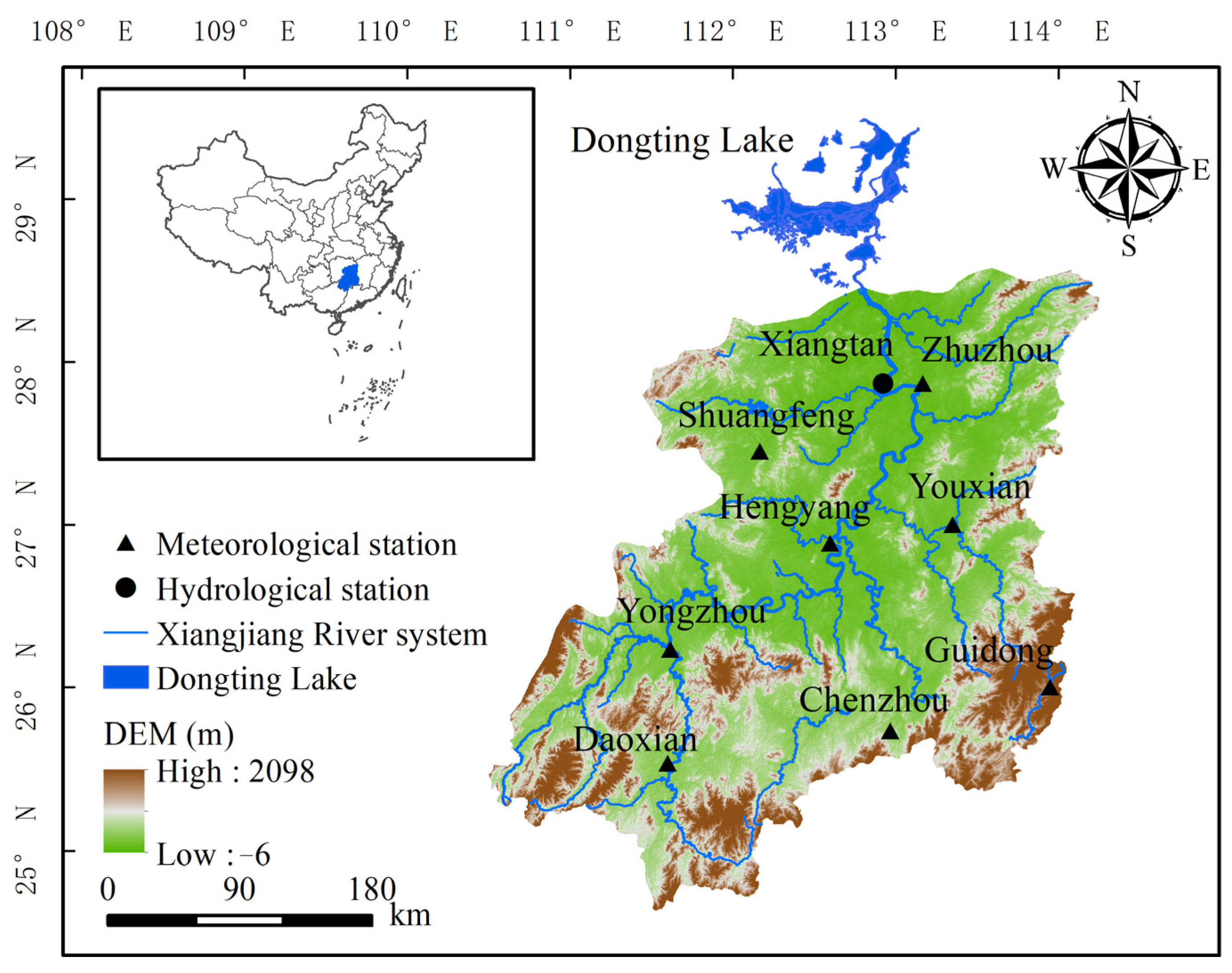
2.1. Study Area Overview

The XJR (110°50′–114°25′ E, 24°5′–28°25′ N) is located in the hilly region of southeast China and is the largest tributary of the Dongting Lake system, as well as a first-class tributary of the Yangtze River (Figure 1). The watershed has abundant precipitation and a dense network of rivers, with a total length of 856 km on the main stream and an asymmetrical feather pattern of tributaries on both sides of the river. The recharge source of flow is mainly rainfall, which is influenced by its spatial and temporal distribution, and, in its natural state, the flow in the XJR basin is very unevenly distributed within the year. As a result, a large number of reservoirs have been built on its main tributaries. But, this has also led to significant changes in the natural hydrological situation of the XJR, which has largely affected the habitat and biological abundance of the wetlands of the XJR basin and Dongting Lake.

2.2. Data Source and Processing

In this research, meteorological data from eight national meteorological stations in the XJR basin and flow data from the XJR basin’s hydrological control station (Xiangtan Station) were selected (Table 1 records the basic information of the relevant stations). In particular, weather station data (including wind speed, relative humidity, temperature, sunshine hours, and precipitation) are provided by the China Meteorological Data Service Center (http://data.cma.cn/, accessed on 16 March 2022). The flow data from the Xiangtan station is obtained from the Yangtze River Basin Hydrological Yearbook. The potential evapotranspiration was calculated for each meteorological station using the Penman–Monteith formula [27]. The Thiessen polygon principle was also used to calculate the precipitation and potential evapotranspiration for the whole basin [28]. In addition, most neural network models require normalized pre-processing of the dataset before simulation. In this paper, the original dataset is pre-processed using a normalization formula to ensure fast and stable convergence of the model, while the normalized output is subjected to a corresponding denormalization operation; the specific steps can be found in [29]. The land-use data used in the InVEST model (1990, 1995, 2000, 2005, 2010, 2015, and 2020) were derived from the Data Center for Resources and Environmental Sciences of the Chinese Academy of Sciences (http://www.resdc.cn, accessed on 16 March 2022).

3. Methodology

3.1. Hydrological Variability Determination

The Mann–Kendall trend test determines whether there is a significant trend change in the time-series data. In this study, the Mann–Kendall trend test was used to calculate three series of flow, precipitation, and potential evapotranspiration in the Xiangjiang River basin, and the specific principles can be found in [30]. When the statistic Z < 0 indicates that the series shows a decreasing trend, Z > 0 indicates that the series shows an increasing trend, and, when |Z| > 1.96, it indicates that the series trend passes the 95% significance test. Meanwhile, to analyse the variation of flow series more intuitively, we determined the mutation years of the flow series using the Sliding t-test and the Cumulative Anomaly test [31].

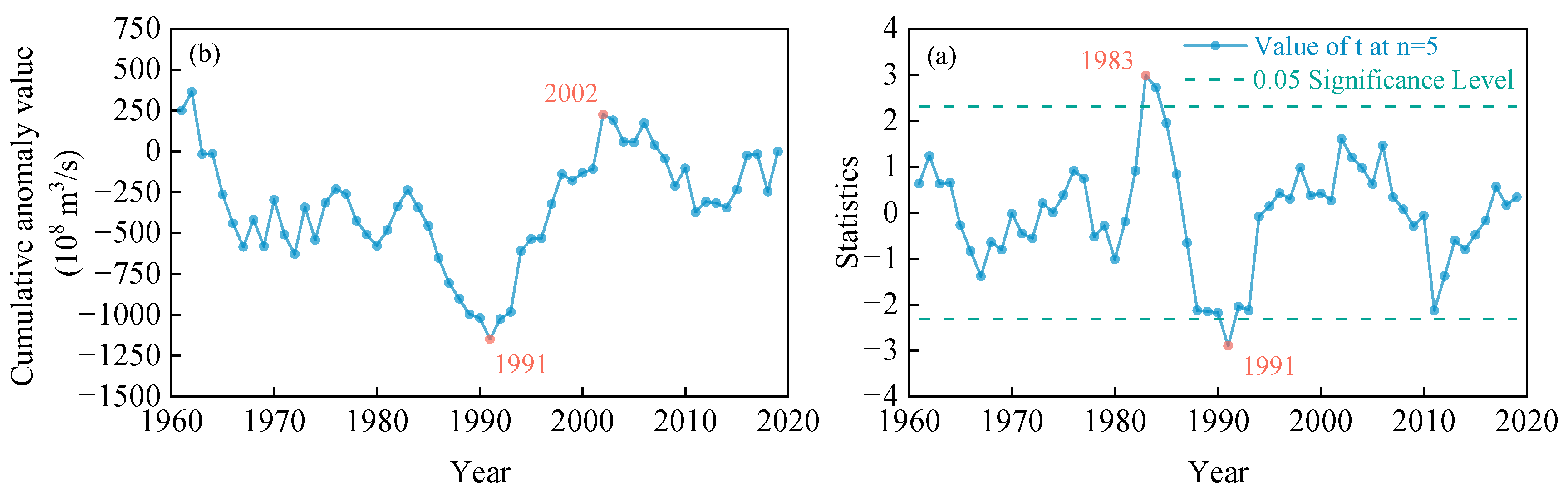
3.1.1. Sliding t-Test

Sliding t-test is widely used in the analysis of hydrological time-series mutability. The method tests for mutation points by examining whether the difference between the means of the two sample groups is significant. For the time-series (x), there are a total of n sample sizes, with a certain moment as the reference point. The samples of the sequence x1 and x2 before and after the base point are n1 and n2, respectively, with mean x 1 ¯ and x 2 ¯ (in m3/s) and variance s 1 2 and s 2 2 (in m6/s2). Then, the statistics are as follows:
t = x 1 ¯ x 2 ¯ s × 1 n 1 + 1 n 2
of which
s = n 1 s 1 2 + n 2 s 2 2 n 1 + n 2 2

3.1.2. Cumulative Anomaly Test

The principle of the Cumulative Anomaly test is to accumulate the difference between each data point and the mean of the series in order to determine the year of mutation. Due to its simple structure and easy implementation, this method has been widely used in the field of hydrology. For a flow series Q, the cumulative distance level xt at any moment t is expressed as follows:
x t = i = 1 t ( Q i Q ¯ )
where Qi is the value of the ith time-period of the flow series, Q ¯ is the mean value of the flow series, and the units of the parameters are m3/s.

3.2. The Most Ecologically Relevant Hydrological Indicators

3.2.1. The Indicators of Hydrologic Alteration

To better evaluate the hydrological situation of a basin, Richter et al. [32] developed 33 Indicators of Hydrologic Alteration (IHA) in terms of flow, time, frequency, delay, and rate of change. Based on the IHA indicator, Richter proposed a method to quantify the extent of change in the IHA indicator following hydrological disturbance, the Range of Variability Approach (RVA). It is calculated as follows:
D i = N 0 , i N f N f × 100 %
D 0 = ( 1 32 i = 1 32 D i 2 ) 0.5
where Di indicates the degree of change in the ith hydrological indicator (when Di is at 0–33%, it is considered a low degree of change; when Di is at 33–67%, it is considered a moderate degree of change; and when Di is at 67–100%, it is considered a high degree of change); N0,i indicates the number of years in which the ith hydrological indicator falls within the RVA target threshold after hydrological variation; Nf indicates the number of years that the IHA value is expected to be at the RVA target threshold after hydrological variation; and D0 is the degree of change in the combined hydrological indicators.

3.2.2. The Environmental Flow Components

Extreme flows, including high-flow events and low-flow events, are considered necessary to maintain the health of river ecosystems. The Environmental Flow Components (EFCs) are based on this and consist of five flow processes: low flows, extreme low flows, high-flow pulses, small floods, and large floods, with a total of 34 hydrological indicators [33]. The EFCs indicators were evaluated by conducting calculations before and after the disturbances and using coefficients of variation (C). The Ci mainly reflects the degree of variation of the ith indicator from the mean value and is calculated as follows:
C i = S m
where S is the standard deviation before and after hydrological variation, and m is the mean value before and after hydrological variation. The overall change in the coefficients of variation of the EFCs indicator is calculated using the principle of calculating the overall degree of change using the weighted average of the IHA indicators above (Equation (2)).

3.2.3. Principal Components Analysis

Principal Components Analysis (PCA) is a statistical method for multivariate analysis, the basic principle of which is to reduce the dimensionality of a large number of relevant variables into a few uncorrelated variables using orthogonal transformations, and to retain as much information as possible [34]. The principles for determining the number of principal components n are the following: (1) a cumulative contribution of 70–90% and (2) an eigenvalue ≥ 1. The Indicators of Hydrologic Alteration and Environmental Flow Components indicators were screened separately using PCA. And, finally, the most Ecologically Relevant Hydrological Indicators-the Indicators of Hydrologic Alteration (ERHIs-IHA) and the most Ecologically Relevant Hydrological Indicators-the Environmental Flow Components (ERHIs-EFCs) were obtained. They are used to evaluate hydrological situation and environmental flows separately.

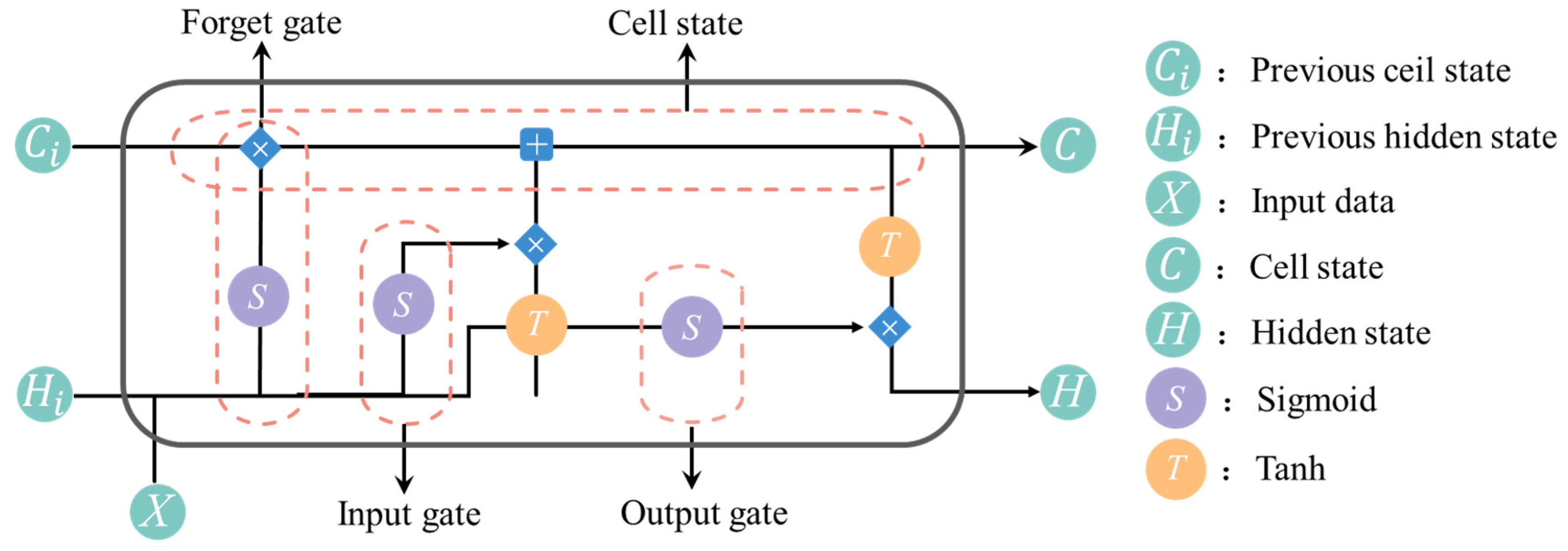
3.3. The Long Short-Term Memory Model

3.3.1. Model Structure

The LSTM model is a variant of the Artificial Neural Network (ANN) model, whose special design structure (cell state and “gate” structure) allows it to avoid the problem of long-term dependency in long-time sequence prediction. Figure 2 reflects a schematic representation of the operation and structure of the LSTM, the details of which can be found in [35]. The study refers to the basin meteorological flow model proposed by Gauch et al. [36]. In this research, natural flows were reconstructed using measured data (including precipitation, potential evapotranspiration, temperature, sunshine hours, wind speed, relative humidity, etc.) from meteorological stations in the basin as the input. The NSE, R2, and RMSE were used as evaluation indicators (Equations (4) and (5)).
N S E = 1 i = 1 n Q o b s , i Q s i m , i 2 i = 1 n Q o b s , i Q o b s ¯ 2 ; R M S E = i = 1 n ( Q o b s , i Q s i m , i ) 2 n
R 2 = Q o b s , i Q o b s ¯ i = 1 n Q s i m , i Q s i m ¯ 2 i = 1 n Q o b s , i Q o b s ¯ 2 i = 1 n Q s i m , i Q s i m ¯ 2

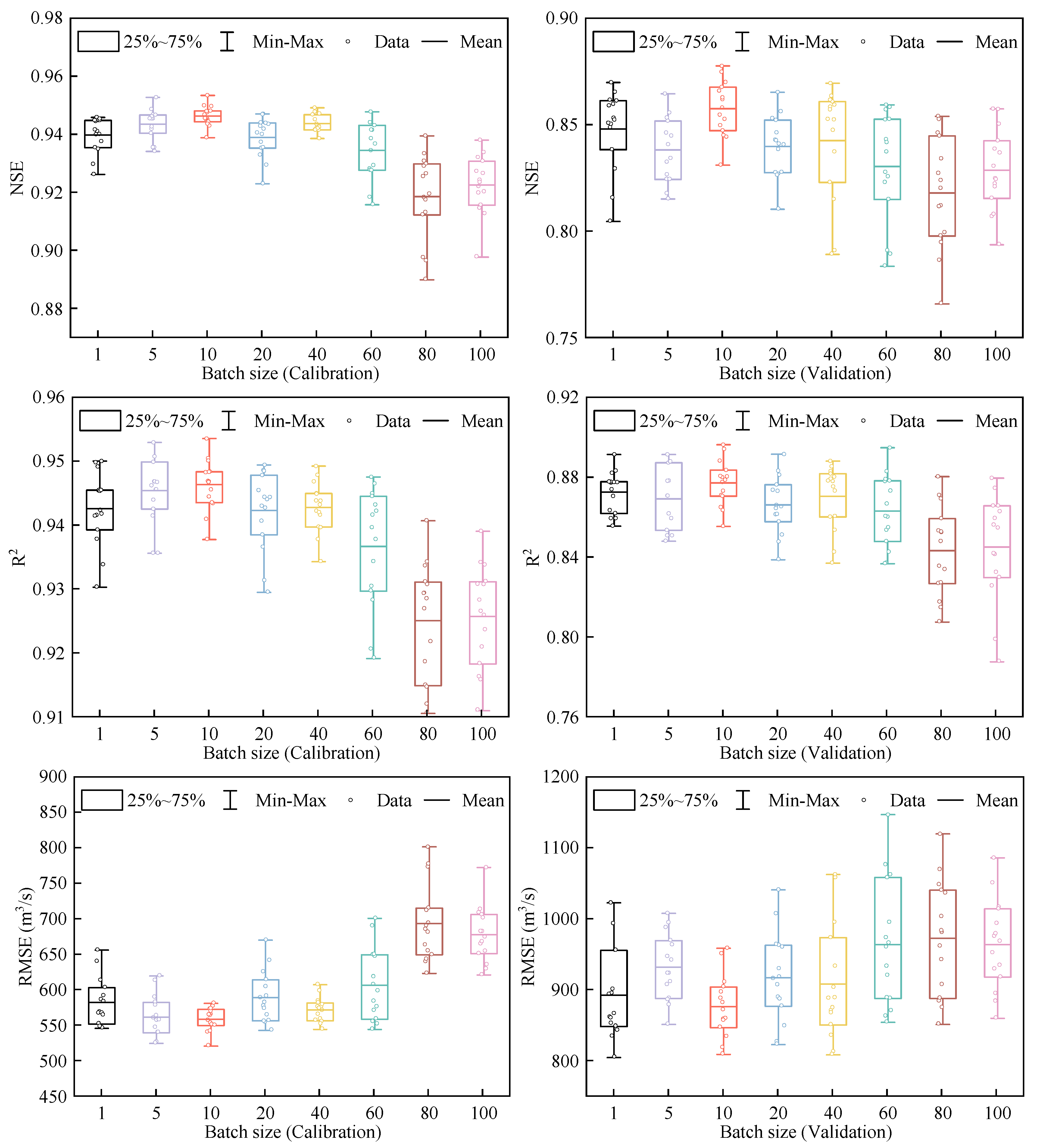
3.3.2. Model Parameters

To better train the LSTM model, the model parameters suitable for the watershed in question were determined. This research refers to the study of Yin et al. [37], which took the 1961–1969 sequence of the XJR basin as the base period and further divided it into a calibration period (1961–1966) and a validation period (1967–1969). The LSTM model contains many important hyperparameters, including hidden size, epoch, dropout rate, batch size, etc., that usually need to be optimised before the model can be learned. In this study, we first determined the hidden size in the hidden layer, and, through training, we found that the model worked best with 150 neurons. As for the epoch, this study first set a longer epoch (200 times), and, after several training sessions, the best fit was found to be after 150 times, thus setting the epoch to 150 times. And, to prevent overfitting problems during the simulation, a discard layer was set up in the study, with a discard probability of 0.4, which meant that there was a 60% probability that the hidden units in this layer would be retained. In addition, it has been shown that the batch size has an impact on the prediction accuracy of the model. Therefore, we set up eight groups of batch sizes (1 d, 5 d, 10 d, 20 d, 40 d, 60 d, 80 d, and 100 d) to train the XJR meteorological streamflow model 15 times, respectively, and used NSE, R2, and RMSE as the evaluation indicators. The model’s results for the calibration and validation periods are shown in Figure 3, and it can be observed that the simulation works best at a batch size of 10 d.
Ultimately, the main model parameters were set as shown in Table 2. The results of the meteorological streamflow model’s reconstructions for the XJR streamflow all follow these parameters. Figure 4 shows the overall effect of the streamflow reconstruction by the model. The observed and simulated streamflow series between 1961 and 2019 reached an R2 of 0.85 and an NSE of 0.84; in the natural period (1961–1990) and in the variation period (1991–2019), the R2 was 0.88 and 0.82, respectively, and the NSE was 0.86 and 0.82, respectively. These results indicate that the LSTM model performs well and can effectively capture the characteristics of streamflow variability.

3.3.3. Separation Framework

Based on the streamflow series simulated by the meteorological streamflow model, an “observation–simulation” comparative analysis was used to quantify the effects of human disturbances and climatic factors on hydrological changes [38]. First, the degree of change (D) for the ERHIs-IHA indicator and the change in the coefficients of variation (CV) for the ERHIs-EFCs indicator were calculated for the measured and simulated series, respectively. Assuming that human disturbance and climatic effects are independent of each other, the degrees of change (Dobs) of the observed flow’s hydrological situation and the change in the coefficients of variation (CVobs) of environmental flows are as follows:
D o b s = D h + D c
C V o b s = C V c + C V h
The simulated streamflow is streamflow under the influence of only climate change; thus, the degree of change (Dsim) of the simulated streamflow’s hydrological situation and the change in the coefficients of variation (CVsim) of the environmental flow are as follows:
D s i m = D c
C V s i m = C V c
The difference between the D values of the observed and simulated sequences and the difference between the observed and simulated CV values are as follows:
D h = D o b s D s i m
C V h = C V o b s C V s i m
The contribution of human disturbances and climatic factors to the hydrological situation and environmental flows, respectively, are the following:
η h = D h D c + D h × 100 % ;     η c = D c D c + D h × 100 %
η V h = C V h C V c + C V h × 100 % ;     η V c = C V c C V c + C V h × 100 %
In the above equations, Dobs and CVobs indicate the degree of variation in the observed ERHIs-IHA indicators and the change in the coefficient of variation of the ERHIs-EFCs indicators, respectively. Dsim and CVsim indicate the degree of variation in the simulated ERHIs-IHA indicators and the change in the coefficient of variation of the ERHIs-EFCs indicators, respectively. Dh and Dc indicate changes in ecohydrological situation due to human disturbance and climatic factors, respectively. CVh and CVc indicate changes in environmental flows due to human disturbance and climatic factors, respectively. ηh and ηc indicate the contribution of human disturbances and climatic factors to changes in hydrological situation, respectively. ηVh and ηVc indicate the contribution of human disturbances and climatic factors to changes in environmental flows, respectively.

3.4. The Integrated Valuation of Ecosystem Services and Tradeoffs Model

The “Habitat Quality” module of the Integrated Valuation of Ecosystem Services and Tradeoffs (InVEST) model was used to assess habitat quality in the XJR basin. This module uses land-use data to reflect the impact of human activity on the environment: the higher the intensity of human activity, the greater the threat to the habitat and the lower the quality of the habitat. Therefore, the relevant parameters (Table 3 and Table 4) were set with reference to relevant studies [39].

3.5. Grey Correlation Theory

Grey correlation analysis is a method of multi-factor statistical analysis that is mainly used to study the degree of correlation between series. The basic idea is to determine whether sequence curves are closely related according to their geometric similarity. The higher the geometric similarity between the sequence curves, the greater the correlation between the corresponding data sequences, thus achieving a quantitative description of the operation process and evolution of the system [40]. The method is based on uncertain information and can effectively measure the degree of association in order to grasp the main characteristics of things to use; it is widely used in the field of hydrology. This study used a grey correlation model to reveal the correlation between the hydrological changes (hydrological situation and environmental flows) and the habitat quality in the XJR basin.

3.6. Shannon Index

Hydrologic changes often impact aquatic organisms, and the Shannon Index (SI) is often used to reflect the evaluation of watershed biodiversity. Yang et al. (2008) [41] established the best-fit relationship between the IHA metrics and the Shannon Index, which has been widely used for evaluating rivers’ biodiversity. In this paper, due to the lack of data on the number of riverine biomes and species in the Xiangjiang River Basin, it is not possible to directly calculate the SI indicators; therefore, by using the relationship equation constructed by Formula (17) for SI and hydrological indicators, it is then possible to initially, roughly assess the biodiversity of the river.
S I = D min / Q min 7 + D min Q 3 + Q 5 + Q min 3 + 2 × Q max 3 + R r a t e
where Dmin is the Julian date of the annual minimum daily flow; Q3 and Q5 are the average monthly flows in March and May, respectively; Qmin3 and Qmin7 are the annual minimum 3-day flow and the annual minimum 7-day flow; Qmax3 is the annual maximum 3-day flow; and Rrate is the overflow rate.

4. Results

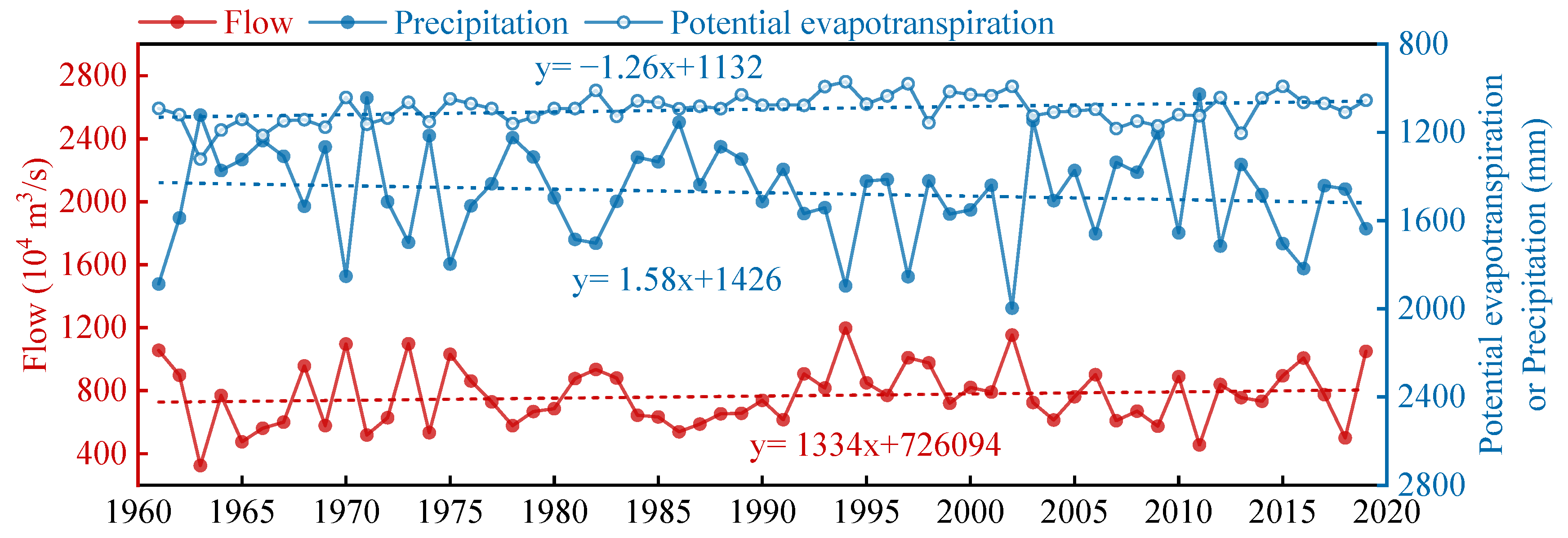
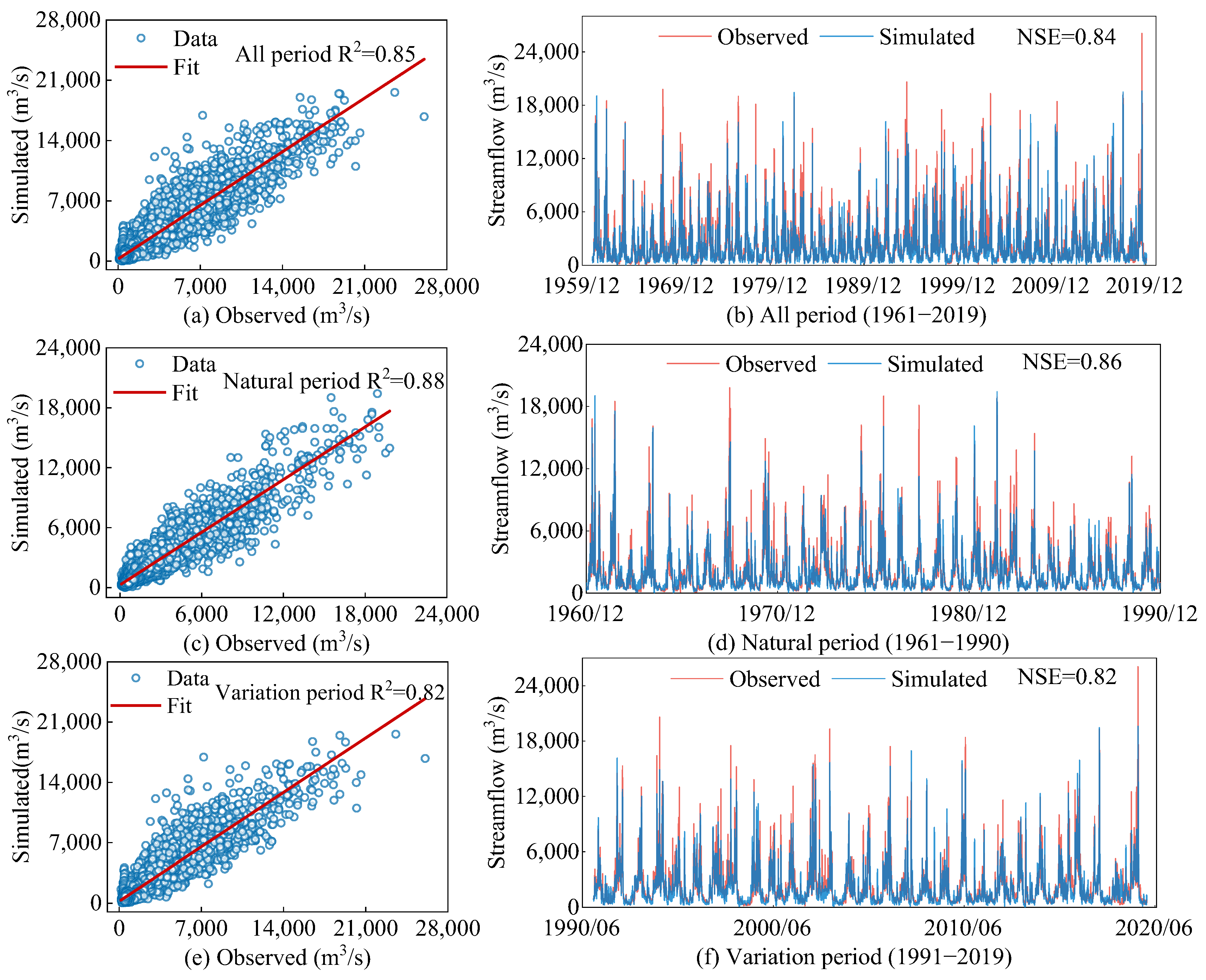
4.1. Trend and Mutation Analysis

The study conducted a Mann–Kendall trend test for annual flow, annual precipitation, and annual potential evapotranspiration in the XJR basin (Table 5). The statistics (Z) for the annual flow and precipitation were 1.11 and 1.23, respectively, both of which failed the 95% significance level test, also indicating that the annual flow and the annual precipitation in the XJR are on an upward, but not significant, trend. The annual flow’s and annual precipitation’s rate of rise were 1334 (m3/s)/Year and 1.58 mm/Year, respectively (Figure 5). In contrast, the annual potential evapotranspiration statistic (Z) was −2.41, which passed the 95% significance level test, indicating a significant decrease in the annual potential evapotranspiration in the XJR basin; its rate of decrease was −1.26 mm/Year. Based on the Sliding t-test and Cumulative Anomaly test used to analyse the mutation years of the XJR flow (Figure 6), the mutation point detected by both tests, together, was 1991. This research thus takes 1991 as the year of sudden hydrological change in the XJR and divides the flow sequence (1961–2019) into a natural period (1961–1990) and a variation period (1991–2019).

4.2. The Most Ecologically Relevant Hydrological Indicators

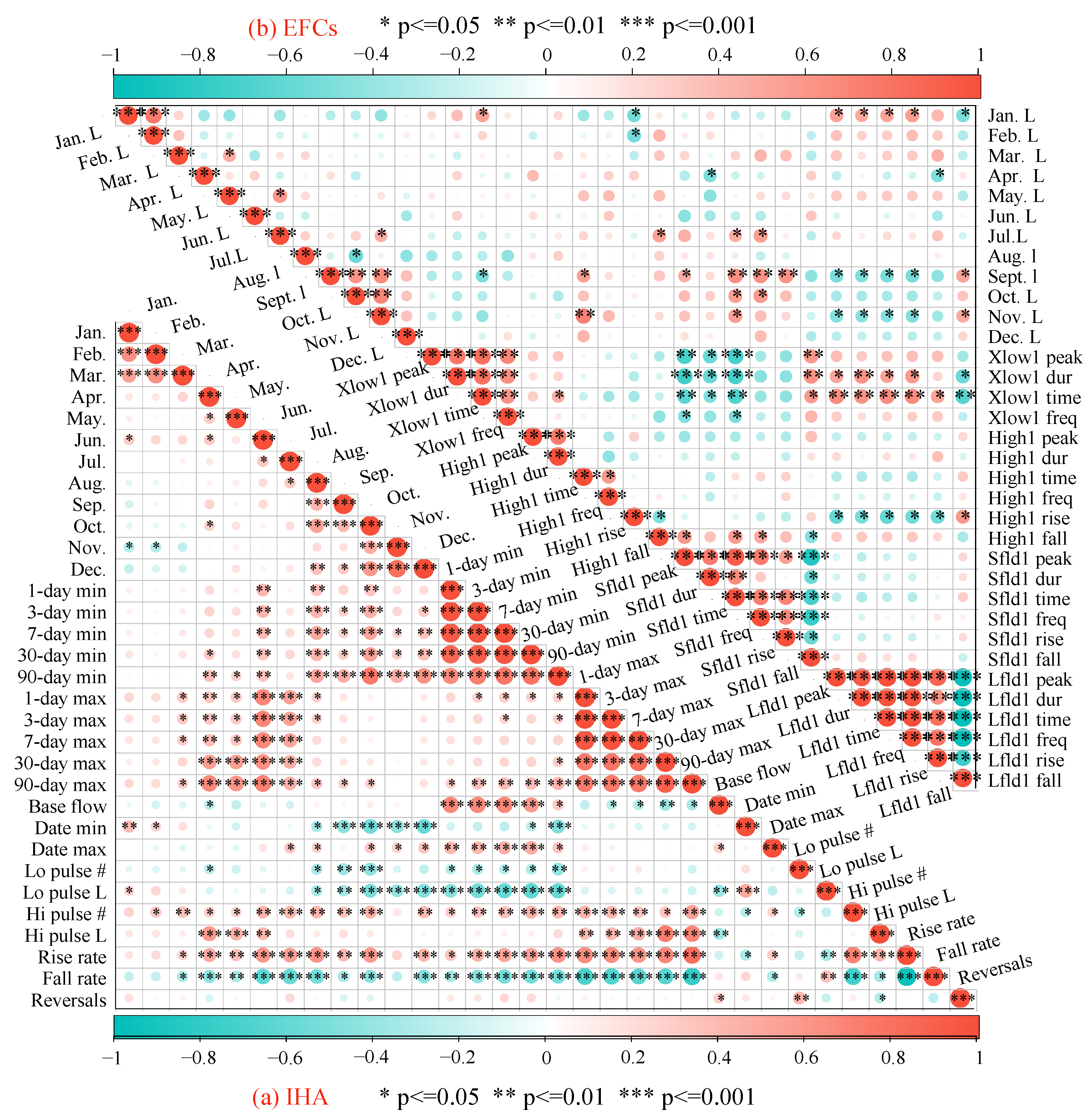
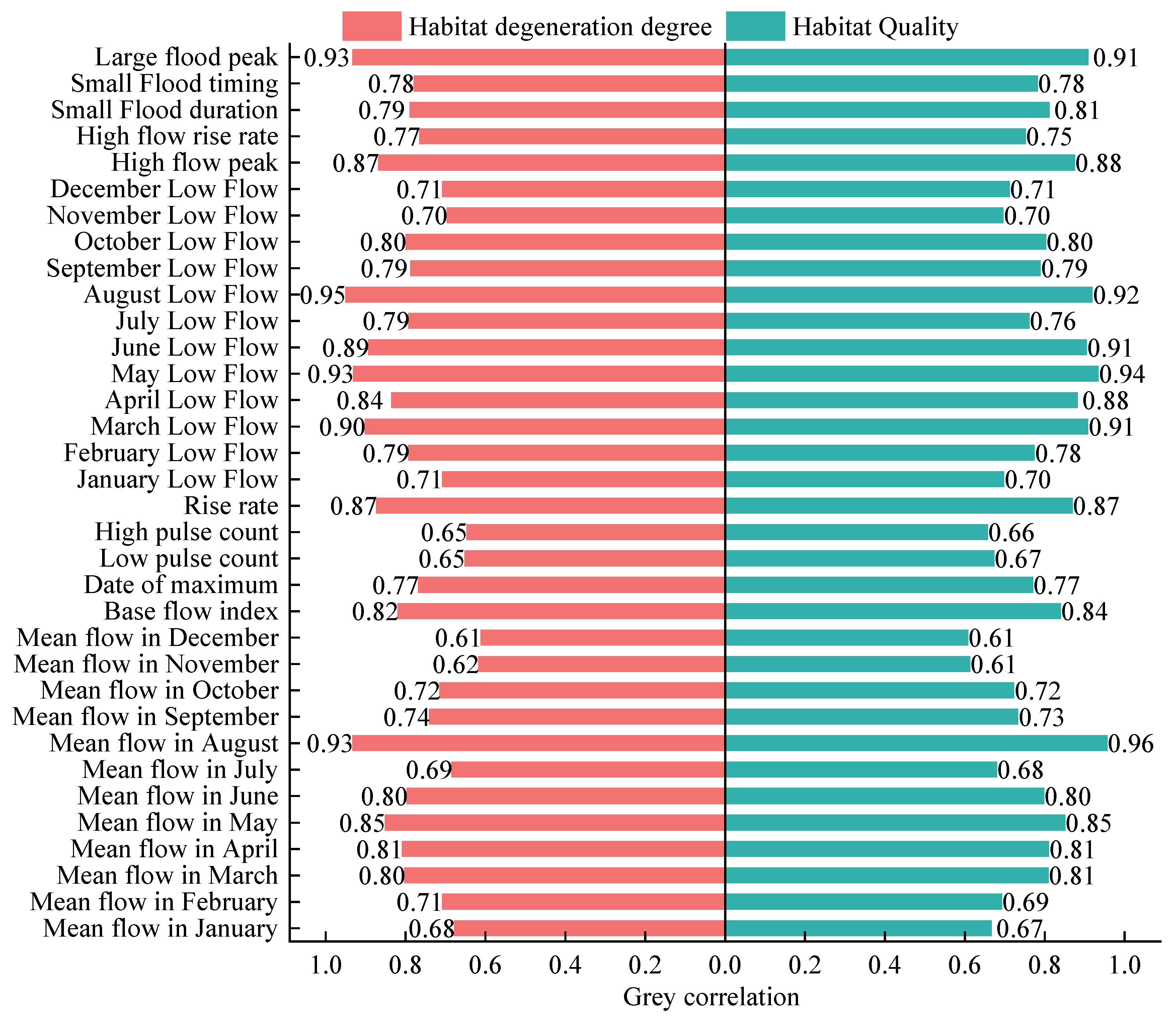
4.2.1. Correlation Analysis of Indicators and Selection of ERHIs

The correlation between the 32 IHAs and between the 34 EFCs was analysed based on the Pearson correlation coefficients. And, Figure 7 reflects the high sink residual and strong correlation between both indicators, like between the annual minimum flows (1, 3, 7, 30, and 90 day), between the time of occurrence and the number of major floods, etc. Thus, the ERHIs in this study were selected from the IHAs and the EFCs using PCA. Figure 8a,b show the eigenvalues and cumulative contributions of the IHA and the EFCs at Xiangtan Station, respectively. From Figure 8a, it can be observed that the eigenvalues of the first seven principal components of the IHA indicators for the XJR basin are all greater than one and have a cumulative contribution of about 80%. From Figure 8b, it can be found that the eigenvalues of the first nine principal components of the XJR basin’s EFCs indicators are all greater than one, and the cumulative contribution is about 80%. Based on the principle of principal component extraction, the PC1–PC7 in Figure 8a were selected as the main components of the required IHA indicators. And the PC1–PC9 in Figure 8b were selected as the main components of the required EFCs indicators in this study. In addition, a factor loading matrix of the principal components was calculated to further screen the ERHIs, with the criterion that the indicator with the highest or higher absolute value of the loading was used as the ERHIs. A month’s flow may be correlated to the previous month’s flow, but, as the 12-month average and low flows reflect the intra-year course of human and ecosystem water availability in a given month, we added these indicators to the ERHIs. The final screening of the ERHIs can be seen in Table 6.

4.2.2. Inter-Annual Variation in ERHIs Indicators

The inter-annual variability of the screened ERHIs indicators was studied based on the observed flow series (Figure 9). In terms of the temporal characteristics of the ERHIs-IHAs, only April, May, and October saw a decrease in the mean flow (rates of 20.86 (m3/s)/year, 11.30 (m3/s)/year, and 0.20 (m3/s)/year, respectively). The remaining monthly average flows showed an upward trend, with more pronounced increases in January, March, and July (rates of 11.07 (m3/s)/year, 12.90 (m3/s)/year, and 17.17 (m3/s)/year, respectively). The base flow index showed a slight increase (0.0015); the date of maximum had a delay; and the flow rate’s rise rate was increasing at a rate of 0.69 m3/s/d per year. In addition, the low pulse count and high pulse count showed an increasing trend. For the ERHIs-EFCs, the monthly low flows only showed a decreasing trend in October (at a rate of 1.63 (m3/s)/year), while remaining monthly low flows showed an increasing trend. The high flow’s rise rate was increasing at a rate of 1.41 m3/s/d per year. The small flood duration was extended and the small flood timing was delayed. In addition, the large flood peak increased significantly at a rate of 69.20 m3/s per year, but the high-flow peak decreased at a rate of 7.65 m3/s per year. These two indicator changes indicate that flows in the XJR basin have increased in many ways.

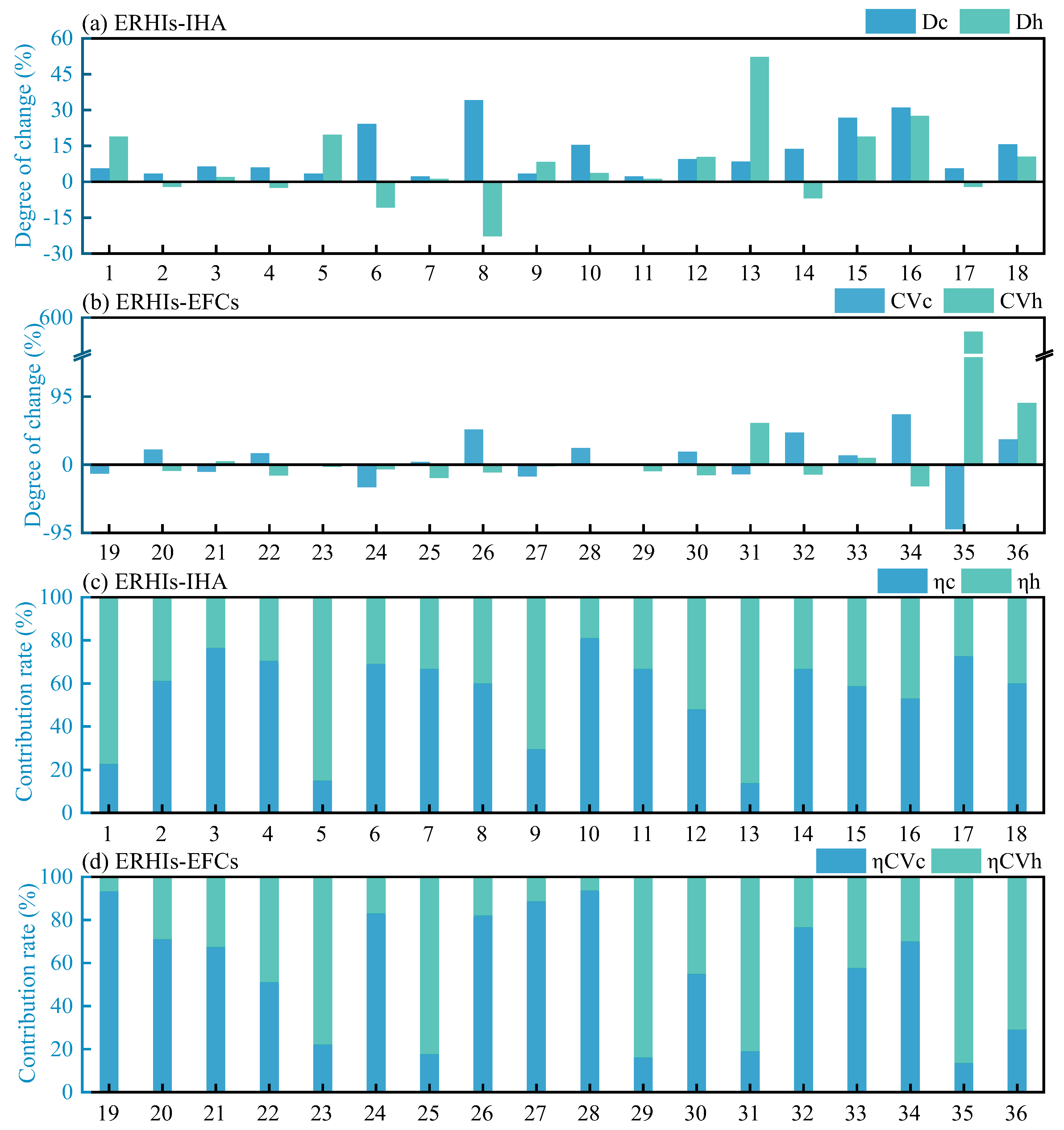
4.3. Ecohydrological Situation, Environmental Flow Evolution, and Quantitative Attribution

A meteorological streamflow model was used to reconstruct the natural flow of the XJR under the influence of climatic factors only and was combined with measured flows to calculate the ERHIs-IHA and the ERHIs-EFCs. Table 6 reflects the changes in the observed flow before and after hydrological variation while giving the degree of change (ERHIs-IHA) and the change in the coefficients of variation (ERHIs-EFCs) calculated based on the observed (obs) and simulated (sim) flow series. From this, it could be seen that the overall degree of change for the ERHIs-IHA and the overall change in the coefficients of variation for the ERHIs-EFCs obtained based on the measured flow were 26.21% and 121.23%, respectively. The overall degree of change for the ERHIs-IHA and the overall change in the coefficients of variation for the ERHIs-EFCs obtained based on the simulated flow were 15.71% and 35.07%, respectively. We attributed changes in the ERHIs in the XJR based on an “observation–simulation” comparison (Figure 10). Climatic factors contributed more to changes in the ecohydrological situation (60%) and human disturbance was the main driver of changes in the environmental flows (71%).
For the ERHIs-IHA, the base flow index, low pulse count, and high pulse count based on the measured flow all achieved a moderate change, while the three indicators based on the simulated flow showed a low change. Most of the simulated flow’s variability was reduced compared to the measured monthly average flow’s variability. In addition, the measured changes in the date of maximum and the rise rate were 6.90% and 3.45%, respectively, while the simulated flow’s changes increased to 13.79% and 5.55%, respectively. For the ERHIs-EFCs, the variability of monthly dry flows in May–September (except August) and November was lower in the modelled results than in the measured flow’s results. The measured variances for the high flow rise rate and the small flood timing were 31.12% and 40.15%, respectively, while the simulated flow’s variances were even higher (44.88% and 70.19%). From the attribution results, it can also be seen (Figure 10c) that human disturbances contribute more than 50% to the mean low in January, mean flow in May, mean flow in September, mean flow in December, and base flow index (77%, 85%, 71%, 52%, and 86%, respectively), and that climate factors have a greater impact on the remaining ERHIs-IHA (53–81%). For the ERHIs-EFCs (Figure 10d), human disturbance had a greater impact on the changes in the four indicators of May low flow, July low flow, November low flow, high-flow peak, and large flood peak than on climatic factors (78–87%), while, for the other ERHIs-EFCs indicators, the contribution of climate change was more pronounced (51–94%).

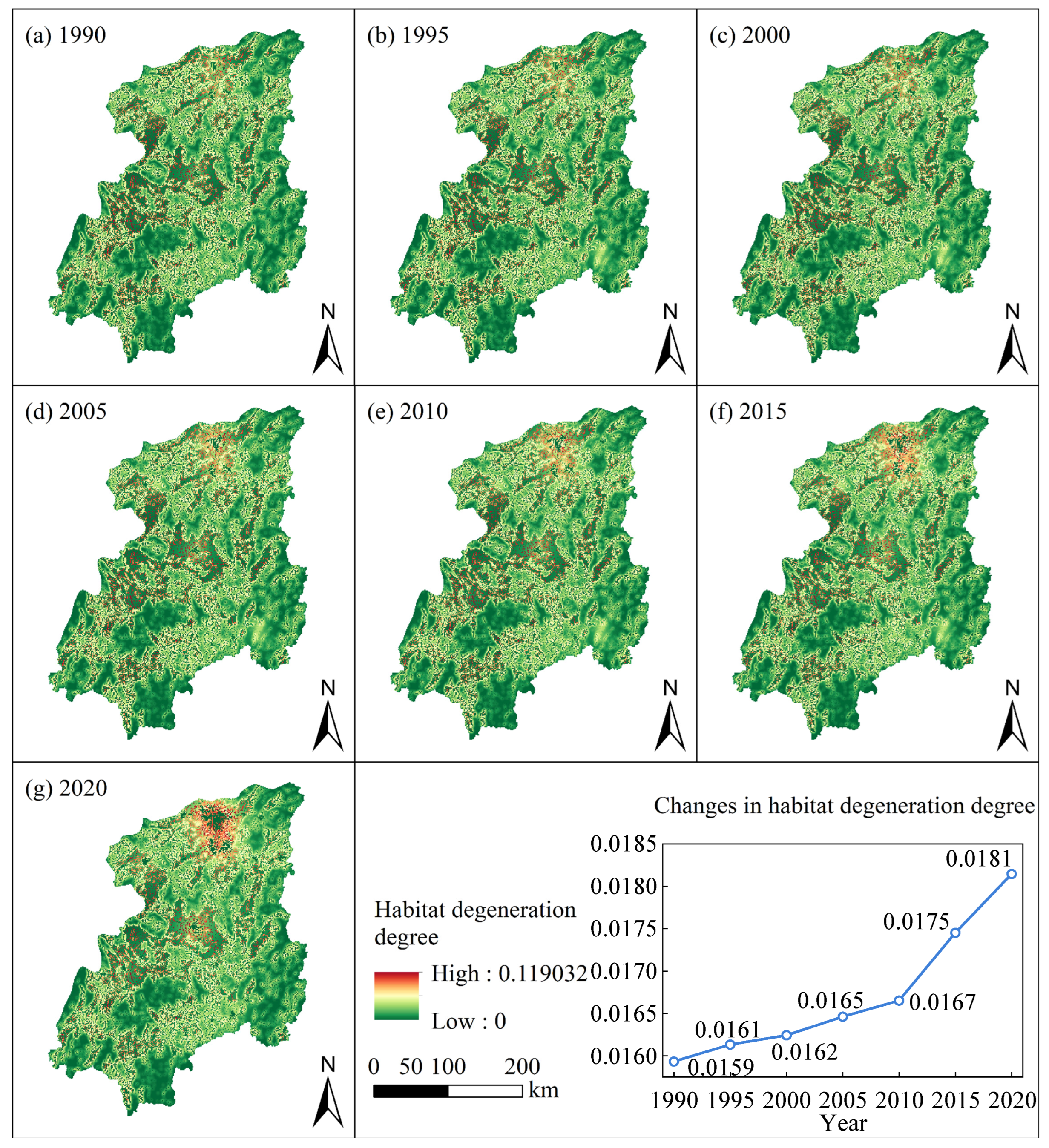
4.4. Habitat Quality Assessment and Its Response to Hydrological Change

The results of habitat degradation and habitat quality distribution in the XJR basin were obtained based on the InVEST model. Figure 11 reflects the spatial distribution of the habitat’s degeneration degree in the XJR basin between 1990 and 2020. The high-degradation areas were concentrated in the middle and lower reaches of the basin, and the high-degradation areas spread to the surrounding areas over time, especially in the cities of Changsha, Xiangtan, and Zhuzhou, during which the average degradation of the basin increased from 0.0159 to 0.0181 (an increase of 13.84%). The maximum degradation increased from 0.1137 to 0.1190 (an increase of 4.66%); the low values of degradation were concentrated in the mountainous areas of the upper part of the basin. The spatial distribution of habitat quality in the XJR basin from 1990 to 2020 (Figure 12) shows that the areas with low habitat quality are also located in the urban areas in the middle and lower reaches of the basin, especially in the axis around Changsha and between Xiangtan and Zhuzhou, and in the Hengyang area in the middle reaches of the basin, while the habitat quality is higher in the Luoxiao Mountains, the Baku Lian Jiu Mountains, the Yangming Mountains, and the Nanling Mountains. In terms of temporal changes, the habitat quality in the XJR basin was on a declining trend between 1990 and 2020, with the average level of habitat quality in the basin decreasing from 0.7698 to 0.7569 (a decrease of 1.68%) during this period. The habitat quality decreased by 0.0004 (0.05%), 0.0007 (0.09%), 0.0015 (0.20%), 0.0009 (0.12%), 0.0041 (0.54%), and 0.0053 (0.70%) in the six periods between 1990 and 2020, respectively, while the area of low habitat quality in the basin gradually expanded to the periphery.
A grey correlation model was constructed from the time-series of habitat degeneration degree, habitat quality, and ERHIs in the XJR basin to quantitatively reveal the impact of hydrological changes on habitat quality (Figure 13). The habitat quality index had a strong correlation with each of the ERHIs (all the correlations were greater than 0.6). Of these, the ERHIs-EFCs were more highly correlated with the habitat’s quality (habitat degeneration degree) than the ERHIs-IHA, overall. For both the habitat quality and habitat degeneration degree, the ERHIs with correlations greater than 0.90 were mean flow in August, March low flow, May low flow, August low flow, and large flood peak. It is also clear from this that habitat quality (habitat degeneration degree) responds more strongly to changes in environmental flows.

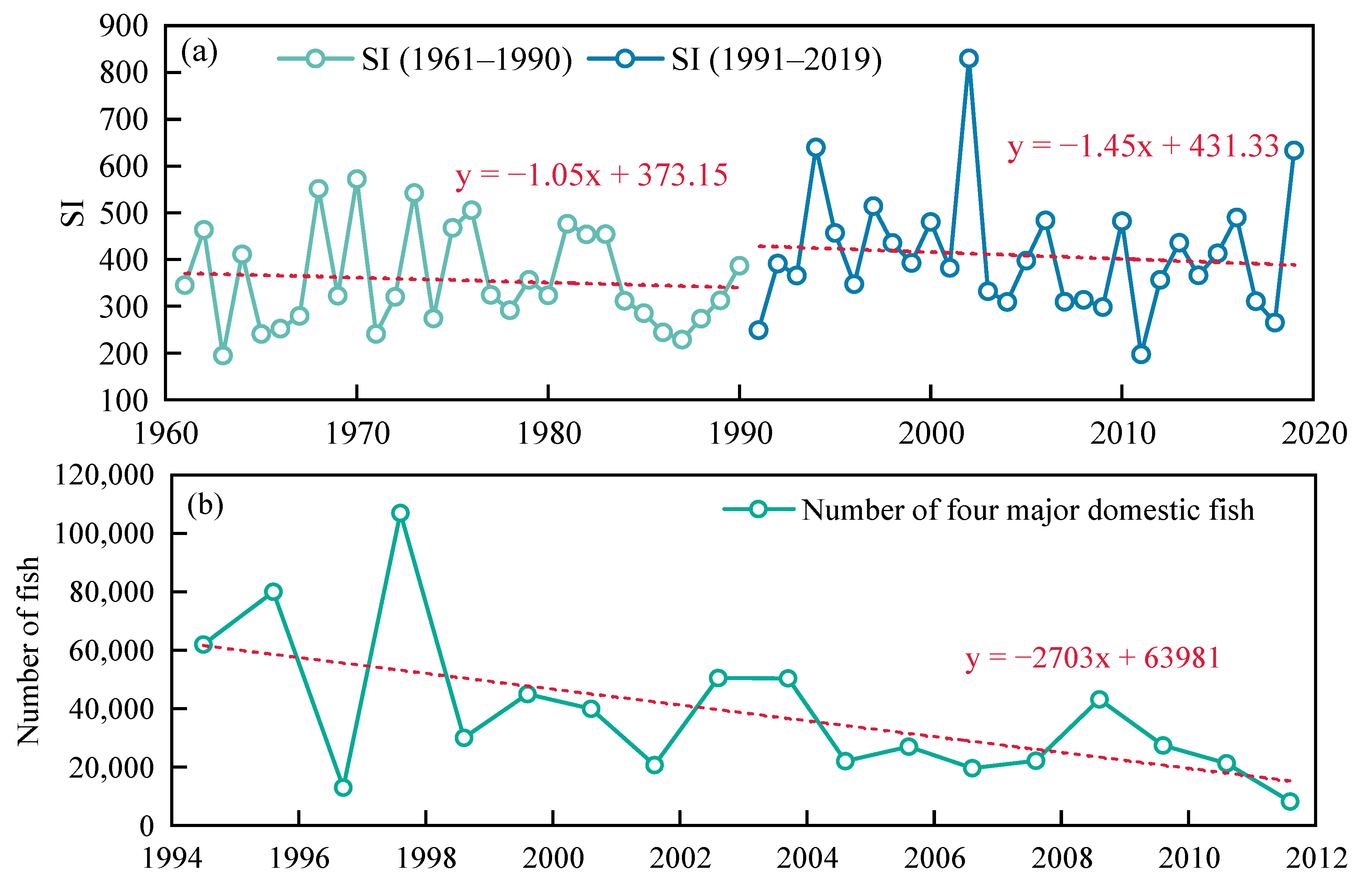
4.5. Riverine Biological Conditions

The study adopted widely used SI indicators to evaluate the river biodiversity of the XJR (Figure 14a) and collected the number of XJR’s four major domestic fish after hydrological variability (Figure 14b) [42,43]. It can be found that, before the hydrological mutation, the decline rate of the SI index in Xiangjiang River was −1.05/year; however, after the mutation, the decline rate of the SI index reached −1.45/year. At the same time, we found that the number of the four major domestic fish in the XJR basin also showed a decreasing trend after the hydrological variability, with a decreasing rate of 2703 fish/year. In addition, from the correlation between the catch of tetras and the ERHIs, we found that several ERHIs metrics showed a strong correlation (greater than 0.65) with them. These indicators were large flood peak, small flood duration, October low flow, June low flow, low pulse count, and mean flow in October.

5. Discussion

Rivers are among the most complex natural ecosystems, and fluctuations in flow in their natural state are considered critical for maintaining the health of watershed ecosystems [44]. However, research found that global environmental change (including climate and land-use change) has profoundly altered the flow patterns of most rivers worldwide. River ecosystems are sensitive to changes in flow [45]. Palmer and Ruhi [46] found that, when flow changes occur, they not only reduce primary productivity but also affect material cycling, ultimately leading to ecological degradation. The XJR, as the mother river of the Hunan Province as well as the largest river in the Dongting Lake system, not only feeds 60% of the provincial population but is also the habitat of many rare plants and animals [47]. This study found that the annual potential evapotranspiration in the XJR basin declined significantly, the precipitation and the flow were on an upward trend in terms of inter-annual variability, and the annual flow changed abruptly in 1991. Based on the measured daily flow of the XJR, the study used PCA to screen Indicators of Hydrologic Alteration and Environmental Flow Components, effectively avoiding information sink between indicators, and finally obtained 34 ERHIs.
It was found that the vast majority of the ERHIs-IHA showed an increasing trend after hydrological variation. After 1991, the average monthly flow increased more markedly in winter and decreased most markedly in spring (except March), which is inextricably linked to the human regulation of river water allocation. The XJR flows significantly less during the flood season, which represents the onset of flow homogenisation, with a reduced flow during the high-flow months and increased in flow during the low-flow months. Tonkin et al. [48] found that this phenomenon can lead to a reduction in organic matter in downstream floodplains, while potentially altering the adaptive range of vegetation habitats and reducing habitat quality. The degree of change in the base flow index, the low pulse count, and the high pulse count were 60.59%, 45.55%, and 58.62, respectively, all reaching a moderate change. And, the increase in the base flow index (from 0.17 to 0.22) had a negative impact on drifting eggs [49]. High and low pulses play an important role in maintaining the compatibility of organisms’ life cycles, and their variation can directly or indirectly affect the population dynamics and structure of aquatic communities in river and floodplain systems [50]. Khatun and Pal [51] found that dam construction in the Tangon River basin resulted in reduced flow velocities in the lower river and a significant reduction in suitable fish habitats. Only two of the ERHIs-EFCs showed a decreasing trend (October low flow and high flow peak), with the high flow peak variation reaching 44.41%, the main reason for this phenomenon being the storage of water in the middle and upper reaches of the reservoir complex during the flood season. After the mutation, most of the monthly low flows were replenished, which effectively restored a certain level of dissolved oxygen and water temperature in the river, which could then provide basic living conditions for organisms [52]. After 1991, the small flood duration was extended from 30.54 d to 38.76 d. The small flood timing was also delayed from late spring to early summer. And, in a study of flooding by Bailly et al. [53], they found that prolonged small flood events may be beneficial in preventing encroachment of riparian vegetation on the river and that their duration is important for the reproduction and survival of fish. These findings were corroborated by our results, where the decline in the SI indicator intensified after hydrological variability, with the rate of decline decreasing from −1.05/year to a rate that would be −1.45/year. Four major domestic fish also showed a downward trend in their abundance (2703 fish/year). In conclusion, the operation of the upper and middle reaches of the XJR reservoir complex changed the hydrological situation and environmental flow composition in the basin, and the spatial and temporal evolution of hydrological processes in their natural state was disrupted. These changes negatively impacted the XJR’s four major domestic fish. Therefore, this study developed a quantitative attribution study for both.
In the study, the human contribution to the change in mean flow in January was found to be 77%, but, for the change in January low flow, the human contribution was only 7%. This reasonably reflects the role of human activities aimed at recharging the dry season, as well as the fact that climatic elements are the primary cause of January low flow. This conclusion is supported by the findings of Guo et al. [54] that the role of human activities in the XJR flow is mainly reflected in the recharge of the downstream flow during the dry season and the release of water during the flood season. For changes in the other ERHIs, it is mostly climatic factors that contribute more. Most annual maximum floods in the XJR occur in April–July, when floods are primarily formed by cyclonic frontal storms, and their spatial and temporal variation characteristics are similar to those of heavy rainfall. Flood regulation efforts in the middle and upper reservoirs have led to a reduction in high flows. Best [55] also found that dam operation reduces high flows and affects fish diversity and floodplain area. The attribution results for the high-flow peak explain this phenomenon well (human interference contributing 81%). However, an increasing trend was observed for the large flood peak, which increased from 19,230 m3/s before hydrological variation to 21,310 m3/s after hydrological variation, with a variation of 490.30%. The increase in the frequency of extreme weather occurrences following the sudden change is the main reason for the dramatic increase in the magnitude of major floods in the XJR. Especially in July 2019, when a mega-flood exceeding the 1-in-50-year event occurred in the lower reaches of the XJR, from Hengshan to Xiangtan, including the 1-in-200-year event at Xiangtan station, with a peak flood flow of 26,060 m3/s, far exceeding the historical measured maximum flow (20,600 m3/s on 18 June 1994).
Human activities affect not only the hydrological changes in rivers, but also the quality of watershed habitats. The habitat quality in the XJR basin was on a declining trend between 1990 and 2020, but was overall at a high level (above 0.75). This is because the XJR basin is mainly composed of forest land (62.55–63.29% of the whole basin), with only (2.89–5.23%) of both building land and water bodies. As a result, areas of high value for habitat quality in the catchment dominate. However, the area of water bodies in the basin has increased from 1312 km2 to 1528 km2 (an expansion of 16.46%), and built-up land has expanded from 1411 km2 to 3400 km2 (an expansion of 140.96%), both of which have had a negative impact on the quality of habitats in the basin, where the expansion of water bodies also reflects the increased construction and operation of reservoirs in the basin. The construction and operation of reservoirs in the middle and upper reaches not only influences changes in river hydrology, but also continuously erodes habitats and causes the continuous fragmentation of habitats. In a study of Amazonian forests, Benchimol and Peres [56] found that man-made dams can reduce local habitat quality and adversely affect biodiversity. The expansion of construction land highlights the rapid urbanisation of the middle and lower reaches of the XJR, leading to the gradual expansion of the areas of lower habitat quality around the built-up areas of the city to the periphery, swallowing up the surrounding areas of higher habitat quality. Berta et al. [57], in their study of the Winike Watershed, found that urbanization poses a threat to and continues to degrade habitat quality. Urbanisation has been accompanied by population build-up, industrial and agricultural development, and a dramatic increase in water consumption in all sectors, putting enormous pressure on the local water-transfer sector, as well as compressing ecological water use and having a greater impact on local habitat quality. The correlation between habitat quality (habitat degeneration degree) and the ERHIs corroborates this finding, and the effect of extreme flow events on habitat quality is greater.
There are also some limitations and potential uncertainties in this study. The LSTM model on which the separation framework in the research is based is a black-box model, and its simulation results are a mapping of independent variables to dependent variables, which has some mechanistic resolution but is weak compared to traditional hydrological models [58]. Despite this, its excellent simulation performance and lightweight computation are still loved by many hydrological researchers. The results of Fan et al. (2020) [59] also demonstrate the reliability of the LSTM model in river flow simulations. Meanwhile, in the past two years, researchers have used LSTM models to construct meteorological flow models to reconstruct natural daily flows, and quantitative attribution studies have been conducted with relevant ecohydrological indicators [60]. This all indicates that the output of the model can be applied to hydrological analysis. In addition, LSTM models are subject to uncertainties, e.g., the model structure, parameter values, and input data can lead to model uncertainty and can affect the simulated flow; model uncertainties are inevitable and we have tried our best to optimize our model. For example, the XJR flow mainly originates from precipitation, so a wider range of influencing factors (including precipitation, temperature, wind speed, sunshine hours, etc.) are adopted in the paper to simulate the XJR flow in order to reduce the impact of model uncertainties on the output results. Also, we introduced relevant evaluation metrics (NSE, RMSE, and R2) to evaluate the simulation effectiveness of the model, and the results also indicate that the constructed meteorological flow model is useful in this basin and can be used for the analysis of river ecohydrology. In addition, the final results are basically consistent with the results of previous studies based on hydrological models [61], which indicates that, although there are some uncertainties and limitations in the models, they have little influence on the results of this article, and the conclusions of this article are scientific and reliable [62].
In summary, the XJR basin is undergoing major ecohydrological changes and the habitat’s quality is deteriorating, which poses a huge challenge to local water resources regulation and ecological conservation. The core of the problem is how to restore the natural flow regime of the river as far as possible while ensuring normal water use for human production and living. This study has analysed the hydrological situation and environmental flows, and the quantitative attribution results, habitat quality, and response to ERHIs can provide a scientific basis for managerial decisions. In addition, the LSTM model is more applicable because of its excellent simulation performance, smaller computational effort, and less data required; meanwhile, the data of the InVEST model are easily available. So, the comprehensive evaluation framework constructed in this study can be easily used to evaluate other watersheds, comprehensively analyse changes in watershed hydrology and habitat quality, and provide a scientific basis for the rational allocation of water resources and ecological restoration in the watershed.

6. Conclusions

This study presents a comprehensive assessment of the XJR basin in terms of four aspects: hydrological situation, environmental flows, drivers, and habitat quality. The annual precipitation and annual flow in the XJR basin showed a non-significant upward trend, but the annual potential evapotranspiration showed a significant downward trend. It was found that human disturbances and frequent climate extremes are inevitably altering the natural flow. Most of the ERHIs showed varying degrees of upward trend after hydrological variation (1991). The overall degree of change of the ERHIs-IHA and the overall change in the coefficients of variation of the ERHIs-EFCs obtained from the measured data reached 26.21% and 121.23%, respectively. And, it was found that the ecohydrological situation of the XJR basin is deteriorating, which has had adverse effects on river organisms. Quantitative attribution results indicated that climatic factors are the main factor influencing the ecohydrological evolution of the XJR, but the role of human disturbance cannot be ignored. The habitat quality in the basin decreased over the period 1990–2020, with high values mainly in mountainous areas and low values mostly in urban areas in the middle and lower reaches, gradually expanding to the periphery. The habitat quality (habitat degeneration degree) in the XJR basin has a strong correlation with each ERHIs and responds more strongly to changes in environmental flows.
The impact of human disturbance and climatic factors on watersheds is a complex issue, and the integrated evaluation framework in this paper may provide new insights for other researchers on watershed analysis. The results of the study show that the ecohydrological situation of the XJR has been significantly disturbed and that the quality of the watershed habitat has been damaged. In order to better maintain the natural hydrological evolution of the XJR and improve the quality of the river basin habitats, we propose the following recommendations. Policy makers need to enhance the basin water allocation capacity, which can be improved by constructing a basin-wide scientific water resource regulation and control system, at the same time accelerating the construction of a water-saving society and improving the efficiency of water resources’ utilization. The relevant water-related departments can also strengthen their joint efforts and properly simulate natural flow events through artificial regulation, especially for environmental flow events.

Author Contributions

Conceptualization, F.H.; data curation, F.H.; formal analysis, F.H.; methodology, F.H.; supervision, W.G., F.H. and H.W.; validation, F.H.; writing original draft, F.H.; writing, review, and editing, F.H. All authors have read and agreed to the published version of the manuscript.

Funding

This work was supported by the National Nature Science Foundation of China (Grant No. 51779094); the Wisdom Introduction Project of Henan Province (GH2019032); the 2023 Special Fundamental Research Project Plan for Higher Education Institutions in the Henan Province (23ZX012); and the North China University of Water Resources and Electric Power for the Master’s Innovation Capacity Enhancement Project (NCWUYC-2023025).

Data Availability Statement

Data will be made available on request.

Conflicts of Interest

The authors declare no conflict of interest.

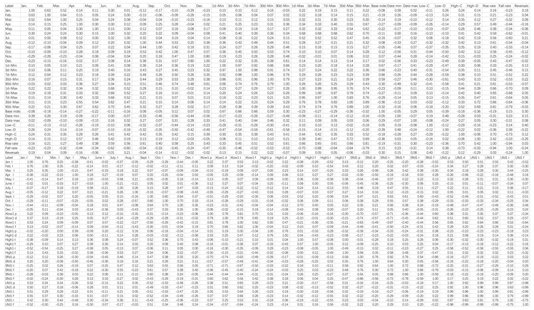
Appendix A. Correlation of Hydrological Parameters

Water 15 03626 i001

References

  1. Karr, J.R. Defining and measuring river health. Freshw. Biol. 1999, 41, 221–234. [Google Scholar] [CrossRef]
  2. Zhou, T. New physical science behind climate change: What does IPCC AR6 tell us? The Innovation 2021, 2, 100173. [Google Scholar] [CrossRef] [PubMed]
  3. Myhre, G.; Alterskjær, K.; Stjern, C.W.; Hodnebrog, Ø.; Marelle, L.; Samset, B.H.; Sillmann, J.; Schaller, N.; Fischer, E.; Schulz, M.; et al. Frequency of extreme precipitation increases extensively with event rareness under global warming. Sci. Rep. 2019, 9, 16063. [Google Scholar] [CrossRef] [PubMed]
  4. Grill, G.; Lehner, B.; Thieme, M.; Geenen, B.; Tickner, D.; Antonelli, F.; Babu, S.; Borrelli, P.; Cheng, L.; Crochetiere, H.; et al. Mapping the world’s free-flowing rivers. Nature 2019, 569, 215–221. [Google Scholar] [CrossRef]
  5. Zhao, H.; He, J.; Liu, D.; Han, Y.; Zhou, Z.; Niu, J. Incorporating ecological connectivity into ecological functional zoning: A case study in the middle reaches of Yangtze River urban agglomeration. Ecol. Inform. 2023, 75, 102098. [Google Scholar] [CrossRef]
  6. Richter, B.D.; Baumgartner, J.V.; Powell, J.; Braun, D.P. A method for assessing hydrologic alteration within ecosystems. Conserv. Biol. 1996, 10, 1163–1174. [Google Scholar] [CrossRef]
  7. Song, X.; Zhuang, Y.; Wang, X.; Li, E.; Zhang, Y.; Lu, X.; Yang, J.; Liu, X. Analysis of hydrologic regime changes caused by dams in China. J. Hydrol. Eng. 2020, 25, 05020003. [Google Scholar] [CrossRef]
  8. Gao, W.; Hu, K.; Gu, Q.; Ling, X.; Ruan, M.; Ren, R. Survey of Fish Resources in Hengyang and Changzhutan Sections of the Main Stream of Xiangjiang River and Measures for Conservation. Low Carbon World 2019, 9, 14–16. [Google Scholar]
  9. Richter, B.D.; Warner, A.T.; Meyer, J.L.; Lutz, K. A collaborative and adaptive process for developing environmental flow recommendations. River Res. Appl. 2006, 22, 297–318. [Google Scholar] [CrossRef]
  10. Gunawardana, S.K.; Shrestha, S.; Mohanasundaram, S.; Salin, K.S.; Piman, T. Multiple drivers of hydrological alteration in the transboundary Srepok River Basin of the Lower Mekong Region. J. Environ. Manag. 2021, 278, 111524. [Google Scholar] [CrossRef]
  11. Olden, J.D.; Poff, N.L. Redundancy and the choice of hydrologic indices for characterizing streamflow regimes. River Res. Appl. 2003, 19, 101–121. [Google Scholar] [CrossRef]
  12. Smakhtin, V.U.; Shilpakar, R.L.; Hughes, D.A. Hydrology-based assessment of environmental flows: An example from Nepal. Hydrol. Sci. J. 2006, 51, 207–222. [Google Scholar] [CrossRef]
  13. Cheng, J.; Xu, L.; Jiang, J. Optimal selection of the most ecologically relevant hydrologic indicators and its application for environmental flow calculation in Lake Dongting. J. Lake Sci. 2018, 30, 1235–1245. [Google Scholar]
  14. Jiang, S.; Zhou, L.; Ren, L.; Wang, M.; Xu, C.; Yuan, F.; Liu, Y.; Yang, X.; Ding, Y. Development of a comprehensive framework for quantifying the impacts of climate change and human activities on river hydrological health variation. J. Hydrol. 2021, 600, 126566. [Google Scholar] [CrossRef]
  15. Arsenault, R.; Martel, J.L.; Brunet, F.; Brissette, F.; Mai, J. Continuous streamflow prediction in ungauged basins: Long Short-Term Memory Neural Networks clearly outperform hydrological models. Hydrol. Earth Syst. Sci. Discuss. 2022, 2022, 1–29. [Google Scholar] [CrossRef]
  16. Hu, C.; Wu, Q.; Li, H.; Jiang, S.; Li, N.; Lou, Z. Deep learning with a long short-term memory networks approach for rainfall-runoff simulation. Water 2018, 10, 1543. [Google Scholar] [CrossRef]
  17. Bai, P.; Liu, X.; Xie, J. Simulating runoff under changing climatic conditions: A comparison of the long short-term memory network with two conceptual hydrologic models. J. Hydrol. 2021, 592, 125779. [Google Scholar] [CrossRef]
  18. Fan, H.; He, H.; Xu, L.; Zhang, M.; Jiang, J. Simulation and attribution analysis based on the long-short-term-memory network for detecting the dominant cause of runoff variation in the Lake Poyang Basin. J. Lake Sci. 2021, 33, 866–878. [Google Scholar]
  19. Cao, Y.; Xu, L.; Fan, H.; Mao, Z.; Cheng, J.; Wang, D.; Wu, Y. Impact of climate and human activities on the changes of ecological flow indicators in the Lake Poyang Basin since 1960s. J. Lake Sci. 2022, 34, 232–246. [Google Scholar]
  20. Sharma, A.; Baruah, A.; Mangukiya, N.; Hinge, G.; Bharali, B. Evaluation of Gangetic dolphin habitat suitability under hydroclimatic changes using a coupled hydrological-hydrodynamic approach. Ecol. Inform. 2022, 69, 101639. [Google Scholar] [CrossRef]
  21. Nagendra, H.; Lucas, R.; Honrado, J.P.; Jongman, R.H.; Tarantino, C.; Adamo, M.; Mairota, P. Remote sensing for conservation monitoring: Assessing protected areas, habitat extent, habitat condition, species diversity, and threats. Ecol. Indic. 2013, 33, 45–59. [Google Scholar] [CrossRef]
  22. Zhang, X.; Zhou, J.; Li, M. Analysis on spatial and temporal changes of regional habitat quality based on the spatial pattern reconstruction of land use. Acta Geogr. Sin. 2020, 75, 160–178. [Google Scholar]
  23. Zhang, H.; Li, S.; Liu, Y.; Xu, M. Assessment of the Habitat Quality of Offshore Area in Tongzhou Bay, China: Using Benthic Habitat Suitability and the InVEST Model. Water 2022, 14, 1574. [Google Scholar] [CrossRef]
  24. de Mello, K.; Taniwaki, R.H.; de Paula, F.R.; Valente, R.A.; Randhir, T.O.; Macedo, D.R.; Leal, C.G.; Rodrigues, C.B.; Hughes, R.M. Multiscale land use impacts on water quality: Assessment, planning, and future perspectives in Brazil. J. Environ. Manag. 2020, 270, 110879. [Google Scholar] [CrossRef]
  25. Zeng, C.; Wen, Y.; Liu, X.; Yu, J.; Jin, B.; Li, D. Impact of anthropogenic activities on changes of ichthyofauna in the middle and lower Xiang River. Aquac. Fish. 2022, 7, 693–702. [Google Scholar] [CrossRef]
  26. Wang, H.; Ma, Y.; Hong, F.; Yang, H.; Huang, L.; Jiao, X.; Guo, W. Evolution of Water–Sediment Situation and Attribution Analysis in the Upper Yangtze River, China. Water 2023, 15, 574. [Google Scholar] [CrossRef]
  27. Djaman, K.; O’Neill, M.; Diop, L.; Bodian, A.; Allen, S.; Koudahe, K.; Lombard, K. Evaluation of the Penman-Monteith and other 34 reference evapotranspiration equations under limited data in a semiarid dry climate. Theor. Appl. Climatol. 2019, 137, 729–743. [Google Scholar] [CrossRef]
  28. Faisal, N.; Gaffar, A. Development of Pakistan’s new area weighted rainfall using Thiessen polygon method. Pak. J. Meteorol. 2012, 9, 1–10. [Google Scholar]
  29. Hou, L.; Zhu, J.; Kwok, J.; Gao, F.; Qin, T.; Liu, T.Y. Normalization helps training of quantized lstm. Adv. Neural Inf. Process. Syst. 2019, 32, 1–11. [Google Scholar]
  30. Hamed, K.H.; Rao, A.R. A modified Mann-Kendall trend test for autocorrelated data. J. Hydrol. 1998, 204, 182–196. [Google Scholar] [CrossRef]
  31. Hu, J.; Ma, J.; Nie, C.; Xue, L.; Zhang, Y.; Ni, F.; Deng, Y.; Liu, J.; Zhou, D.; Li, L.; et al. Attribution Analysis of Runoff change in Min-tuo River Basin based on SWAT model simulations, china. Sci. Rep. 2020, 10, 2900. [Google Scholar] [CrossRef] [PubMed]
  32. Richter, B.; Baumgartner, J.; Wigington, R.; Braun, D. How much water does a river need? Freshw. Biol. 1997, 37, 231–249. [Google Scholar] [CrossRef]
  33. Wang, H.; Huang, L.; Guo, W.; Zhu, Y.; Yang, H.; Jiao, X.; Zhou, H. Evaluation of ecohydrological regime and its driving forces in the Dongting Lake, China. J. Hydrol. Reg. Stud. 2022, 41, 101067. [Google Scholar] [CrossRef]
  34. Olsen, R.L.; Chappell, R.W.; Loftis, J.C. Water quality sample collection, data treatment and results presentation for principal components analysis–literature review and Illinois River watershed case study. Water Res. 2012, 46, 3110–3122. [Google Scholar] [CrossRef]
  35. Kühnert, C.; Gonuguntla, N.M.; Krieg, H.; Nowak, D.; Thomas, J.A. Application of LSTM networks for water demand prediction in optimal pump control. Water 2021, 13, 644. [Google Scholar] [CrossRef]
  36. Gauch, M.; Kratzert, F.; Klotz, D.; Nearing, G.; Lin, J.; Hochreiter, S. Rainfall–runoff prediction at multiple timescales with a single Long Short-Term Memory network. Hydrol. Earth Syst. Sci. 2021, 25, 2045–2062. [Google Scholar] [CrossRef]
  37. Yin, H.; Wang, F.; Zhang, X.; Zhang, Y.; Chen, J.; Xia, R.; Jin, J. Rainfall-runoff modeling using long short-term memory based step-sequence framework. J. Hydrol. 2022, 610, 127901. [Google Scholar] [CrossRef]
  38. Ahn, K.H.; Merwade, V. Quantifying the relative impact of climate and human activities on streamflow. J. Hydrol. 2014, 515, 257–266. [Google Scholar] [CrossRef]
  39. Xu, H.; Dong, B.; Gao, X.; Xu, Z.; Ren, C.; Fang, L.; Wei, Z.; Liu, X.; Lu, Z. Habitat quality assessment of wintering migratory birds in Poyang Lake National Nature Reserve based on InVEST model. Environ. Sci. Pollut. Res. 2023, 30, 28847–28862. [Google Scholar] [CrossRef]
  40. Gao, C.L.; Li, S.C.; Wang, J.; Li, L.P.; Lin, P. The risk assessment of tunnels based on grey correlation and entropy weight method. Geotech. Geol. Eng. 2018, 36, 1621–1631. [Google Scholar] [CrossRef]
  41. Yang, Y.C.E.; Cai, X.; Herricks, E.E. Identification of hydrologic indicators related to fish diversity and abundance: A data mining approach for fish community analysis. Water Resour. Res. 2008, 44, 4. [Google Scholar] [CrossRef]
  42. Yang, H.; Shen, L.; He, Y.; Tian, H.; Gao, L.; Wu, J.; Mei, Z.; Wei, N.; Wang, L.; Zhu, T.; et al. Status of aquatic organisms resources and their environments in Yangtze river system (2017–2021). Aquac. Fish. 2023. [Google Scholar] [CrossRef]
  43. Jia, Y.; Wang, L.; Li, S.; Cao, J.; Yang, Z. Species-specific bioaccumulation and correlated health risk of arsenic compounds in freshwater fish from a typical mine-impacted river. Sci. Total Environ. 2018, 625, 600–607. [Google Scholar] [CrossRef] [PubMed]
  44. Sofi, M.S.; Bhat, S.U.; Rashid, I.; Kuniyal, J.C. The natural flow regime: A master variable for maintaining river ecosystem health. Ecohydrology 2020, 13, e2247. [Google Scholar] [CrossRef]
  45. Comte, L.; Olden, J.D.; Tedesco, P.A.; Ruhi, A.; Giam, X. Climate and land-use changes interact to drive long-term reorganization of riverine fish communities globally. Proc. Natl. Acad. Sci. USA 2021, 118, e2011639118. [Google Scholar] [CrossRef]
  46. Palmer, M.; Ruhi, A. Linkages between flow regime, biota, and ecosystem processes: Implications for river restoration. Science 2019, 365, eaaw2087. [Google Scholar] [CrossRef]
  47. Hu, G.; Mao, D.; Li, Z.; Xu, Y. Evolution Processes and Characteristics of Annual Runoff and Sediment in Xiangjiang River from 1951 to 2011. Bull. Soil Water Conserv. 2014, 34, 166–172. [Google Scholar]
  48. Tonkin, J.D.; Merritt, D.; Olden, J.D.; Reynolds, L.V.; Lytle, D.A. Flow regime alteration degrades ecological networks in riparian ecosystems. Nat. Ecol. Evol. 2018, 2, 86–93. [Google Scholar] [CrossRef]
  49. Richter, B.D.; Baumgartner, J.V.; Braun, D.P.; Powell, J. A spatial assessment of hydrologic alteration within a river network. Regul. Rivers Res. Manag. Int. J. Devoted River Res. Manag. 1998, 14, 329–340. [Google Scholar] [CrossRef]
  50. Petsch, D.K. Causes and consequences of biotic homogenization in freshwater ecosystems. Int. Rev. Hydrobiol. 2016, 101, 113–122. [Google Scholar] [CrossRef]
  51. Khatun, R.; Pal, S. Effects of hydrological modification on fish habitability in riparian flood plain river basin. Ecol. Inform. 2021, 65, 101398. [Google Scholar] [CrossRef]
  52. Bordalo, A.A.; Nilsumranchit, W.; Chalermwat, K. Water quality and uses of the Bangpakong River (Eastern Thailand). Water Res. 2001, 35, 3635–3642. [Google Scholar] [CrossRef]
  53. Bailly, D.; Agostinho, A.A.; Suzuki, H.I. Influence of the flood regime on the reproduction of fish species with different reproductive strategies in the Cuiabá River, Upper Pantanal, Brazil. River Res. Appl. 2008, 24, 1218–1229. [Google Scholar] [CrossRef]
  54. Guo, W.; Hong, F.; Yang, H.; Huang, L.; Ma, Y.; Zhou, H.; Wang, H. Quantitative evaluation of runoff variation and its driving forces based on multi-scale separation framework. J. Hydrol. Reg. Stud. 2022, 43, 101183. [Google Scholar] [CrossRef]
  55. Best, J. Anthropogenic stresses on the world’s big rivers. Nat. Geosci. 2019, 12, 7–21. [Google Scholar] [CrossRef]
  56. Benchimol, M.; Peres, C.A. Widespread forest vertebrate extinctions induced by a mega hydroelectric dam in lowland Amazonia. PLoS ONE 2015, 10, e0129818. [Google Scholar] [CrossRef]
  57. Berta Aneseyee, A.; Noszczyk, T.; Soromessa, T.; Elias, E. The InVEST habitat quality model associated with land use/cover changes: A qualitative case study of the Winike Watershed in the Omo-Gibe Basin, Southwest Ethiopia. Remote Sens. 2020, 12, 1103. [Google Scholar] [CrossRef]
  58. Lees, T.; Buechel, M.; Anderson, B.; Slater, L.; Reece, S.; Coxon, G.; Dadson, S.J. Benchmarking data-driven rainfall–runoff models in Great Britain: A comparison of long short-term memory (LSTM)-based models with four lumped conceptual models. Hydrol. Earth Syst. Sci. 2021, 25, 5517–5534. [Google Scholar] [CrossRef]
  59. Fan, H.; Jiang, M.; Xu, L.; Zhu, H.; Cheng, J.; Jiang, J. Comparison of long short term memory networks and the hydrological model in runoff simulation. Water 2020, 12, 175. [Google Scholar] [CrossRef]
  60. Anshuka, A.; Chandra, R.; Buzacott, A.J.; Sanderson, D.; van Ogtrop, F.F. Spatio temporal hydrological extreme forecasting framework using LSTM deep learning model. Stoch. Environ. Res. Risk Assess. 2022, 36, 3467–3485. [Google Scholar] [CrossRef]
  61. Guo, W.; Hong, F.; Ma, Y.; Huang, L.; Yang, H.; Hu, J.; Zhou, H.; Wang, H. Comprehensive evaluation of the ecohydrological response of watersheds under changing environments. Ecol. Inform. 2023, 74, 101985. [Google Scholar] [CrossRef]
  62. Valentukevičienė, M.; Bagdžiūnaitė-Litvinaitienė, L.; Chadyšas, V.; Litvinaitis, A. Evaluating the impacts of integrated pollution on water quality of the trans-boundary neris (viliya) river. Sustainability 2018, 10, 4239. [Google Scholar] [CrossRef]
Figure 1. Location of the Xiangjiang River basin and the distribution of meteorological and hydrological stations.
Water 15 03626 g001
Figure 2. Structure of the Long Short-Term Memory model.
Water 15 03626 g002
Figure 3. Model performance with different batch sizes (1, 5, 10, 20, 40, 60, 80, and 100).
Water 15 03626 g003
Figure 4. Comparison of observed and simulated flows in the Xiangjiang River basin. The left three panels (a,c,e) show the fitted plots of the measured and simulated flows. The three plots on the right (b,d,f) show the variations of the measured and simulated flow rates.
Water 15 03626 g004
Figure 5. Changes in the inter-annual flow, precipitation, and potential evapotranspiration in the Xiangjiang River basin.
Water 15 03626 g005
Figure 6. Mutation test for the Xiangjiang River flow (a) shows the results of the Sliding t-test, and (b) shows the results of the Cumulative Anomaly test.
Water 15 03626 g006
Figure 7. Correlation plots: (a) plot represents the correlation between the 32 IHA indicators and (b) represents the correlation between the 34 EFCs indicators; the specific values can be found in Appendix A. p represents the significant level.
Water 15 03626 g007
Figure 8. Changes in the characteristic values and cumulative contribution of the Xiangjiang River basin.
Water 15 03626 g008
Figure 9. Inter-annual variation in the selected ERHIs (the extent of variation in these ERHIs was greater than 33%).
Water 15 03626 g009
Figure 10. Impact of human disturbance and climatic factors on the ERHIs: (a,b) represent the degree of changes in the hydrological parameters (parameters 1–36, can refer to Table 6) driven by human activities and climate change; and (c,d) represent the contribution rates of human activities and climate change to changes in the hydrological parameters.
Water 15 03626 g010
Figure 11. Distribution of habitat degeneration degree in the Xiangjiang River basin, 1990–2020.
Water 15 03626 g011
Figure 12. Spatial distribution of habitat quality in the Xiangjiang River basin, 1990–2020.
Water 15 03626 g012
Figure 13. Grey correlation between ERHIs and habitat quality (habitat degeneration degree) in the Xiangjiang River.
Water 15 03626 g013
Figure 14. (a) Changes in the Shannon Index and (b) Situation of four major domestic fish in the Xiangjiang River.
Water 15 03626 g014
Table 1. Basic information on hydrological and meteorological stations.
StationStation TypeControl Area (km2)Altitude (m)Longitude (E)Latitude (N)
XiangtanHydrological station81,600.0063.80112.9327.87
Chenzhou 10,601.17368.80112.9725.73
Shuangfeng 11,905.68100.00112.1727.45
Yongzhou 12,826.50172.60111.6226.23
DaoxianMeteorological station16,456.87192.00111.6025.53
Zhuzhou 16,444.2074.60113.1727.87
Guidong 6170.81835.90113.9526.00
Hengyang 9593.82104.90112.6026.88
Youxian 10,166.43115.20113.3527.00
Note: The control area of the meteorological stations in the basin is calculated based on the Thiessen principle.
Table 2. Model’s parameter settings.
Type of ParametersParameter NameSetting
Hyper parametersDropout rate40
Initial learning rate0.02
Epoch150
Batch size10
Layers5
Dropout period40
Hidden size150
Common parametersTraining hardwareCPU
Gradient threshold1
Network solving algorithmadam
Table 3. Threat factors and their stress intensity.
Habitat Threat FactorsMaximum Impact Distance (km)WeightRecession Correlation
Agricultural land40.6Linear
Rural land50.6Exponential
Urban land101.0Exponential
Industrial mining121.0Exponential
Reservoir/Pond60.6Exponential
Table 4. Sensitivity of land-use type to habitat threat factors.
Land-Use TypeHabitat SuitabilitySensitivity
Agricultural LandRural LandUrban LandIndustrial MiningReservoir/Pond
Agricultural land0.30.00.60.80.80.6
Forest land1.00.60.40.60.70.5
Grass land1.00.80.50.40.60.6
Water body0.70.50.30.70.50.7
Built-up land0.00.00.00.00.00.4
Unused land0.40.30.10.10.30.4
Table 5. Results of the test for trends in flow, precipitation, and potential evapotranspiration in the XJR basin.
Study AreaFlowPrecipitationPotential Evapotranspiration
ZTrendZTrendZTrend
Xiangjiang River basin1.11Rise1.23Rise−2.41 *Decline
Note: * is passing the 95% significance level test.
Table 6. Changes before and after mutations in the ERHIs-IHA and ERHIs-EFCs in the Xiangjiang River basin.
ERHIs-IHA (label)Measured average valuesMeasured thresholdsDegree of
change (%)
1961–19901991–2019LowHighObsSim
Mean flow in January (1)8291298297136124.45.55
Mean flow in February (2)1357155968020341.253.45
Mean flow in March (3)2048252796431318.376.40
Mean flow in April (4)38553247226154493.455.96
Mean flow in May (5)431238672435618923.153.45
Mean flow in June (6)378843231940563613.324.14
Mean flow in July (7)21282866940137103.452.30
Mean flow in August (8)14512083759214311.3334.17
Mean flow in September (9)12191333231220711.723.44
Mean flow in October (10)984.51066460150918.9715.36
Mean flow in November (11)1113122343917883.4482.29
Mean flow in December (12)805.21099403137919.789.48
Base flow index (13)0.170.220.130.2160.598.37
Date of maximum (14)156.30182.90121.20191.406.9013.79
Low pulse count (15)5.205.033.257.1645.5526.72
High pulse count (16)6.308.244.308.3058.6231.03
Rise rate (17)363.50409.60251.00476.003.455.55
Overall degree of change (18)————————26.2115.71
ERHIs-IHA (label)Measured average valuesCoefficient of variationDegree of variation (%)
1961–19901991–2019Pre-1991Post-1991ObsSim
January Low Flow (19)84611040.470.4111.6712.58
February Low Flow (20)113611860.300.3312.4621.03
March Low Flow (21)141616410.280.275.159.95
April Low Flow (22)180718360.200.200.6615.76
May Low Flow (23)187019460.140.143.910.87
June Low Flow (24)167519420.220.1438.0331.59
July Low Flow (25)120615000.310.2614.613.968
August Low Flow (26)109613920.240.3438.1948.94
September Low Flow (27)105411520.390.3218.4516.35
October Low Flow (28)9249260.340.4221.4823.06
November Low Flow (29)100410260.450.4010.541.70
December Low Flow (30)8089060.430.443.21617.91
High-flow peak (31)492347110.170.2444.4113.53
High flow rise rate (32)7607810.290.3831.1244.88
Small Flood duration (33)31390.600.7422.6313.06
Small Flood timing (34)150181.60.090.1340.1570.19
Large flood peak (35)19,23021,3100.030.15490.3090.19
Overall variability (36)————————121.2335.07
Disclaimer/Publisher’s Note: The statements, opinions and data contained in all publications are solely those of the individual author(s) and contributor(s) and not of MDPI and/or the editor(s). MDPI and/or the editor(s) disclaim responsibility for any injury to people or property resulting from any ideas, methods, instructions or products referred to in the content.

