Article

Automatic SWMM Parameter Calibration Method Based on the Differential Evolution and Bayesian Optimization Algorithm

1
School of Civil and Hydraulic Engineering, Huazhong University of Science and Technology, Wuhan 430074, China
2
Sichuan Hydraulic Research Institute, Chengdu 610072, China
*
Author to whom correspondence should be addressed.
Water 2023, 15(20), 3582; https://doi.org/10.3390/w15203582
Submission received: 2 September 2023 / Revised: 6 October 2023 / Accepted: 10 October 2023 / Published: 13 October 2023

Abstract

:
In response to the low accuracy exhibited by the Storm Water Management Model (SWMM), we propose an enhanced Differential Evolution and Bayesian Optimization Algorithm (DE-BOA). This algorithm integrates the global search capability of the differential evolution algorithm with the local search capability of the Bayesian optimization algorithm, which enables a more comprehensive exploration of the vector solution space. A comparative analysis of various types of rainfall events is conducted. For model calibration and validation, a drainage subzone in Jinshazhou, Guangzhou City, is selected as the research subject. In total, 20 specific rainfall events are selected, and the DE-BOA algorithm outperforms the manual calibration, the differential evolution algorithm, and the Bayesian optimization algorithm regarding model calibration accuracy. Furthermore, the DE-BOA algorithm exhibits robust adaptability to rainfall events characterized by multiple peaks and higher precipitation levels, with the Nash–Sutcliffe efficiency coefficient values surpassing 0.90. This study’s findings could hold significant reference value for dynamically updating model parameters, thereby enhancing the model simulation performance and improving the accuracy of the urban intelligent water management platform.

1. Introduction

The simulation of dynamic rainfall runoff in urban areas using urban stormwater modeling serves as the cornerstone of research in urban rainwater management. Among these models, SWMM—one of the most extensively employed urban stormwater runoff models [1,2,3,4,5]—simulates and predicts urban rainwater runoff and drainage conditions [6]. As a structurally intricate distributed hydrological model, SWMM contains parameters that lack precise physical definitions in the process of model abstraction and simulation. These parameters, such as the impermeable manning coefficient, the depression storage in impermeable areas, and the minimum infiltration rate, are typically determined based on past experiences and may vary with different environmental factors [7,8,9,10]. Consequently, parameter calibration and validation are typically conducted during the urban stormwater runoff simulation process, to ensure the precision and applicability of the simulation results [11].
The calibration of SWMM parameters primarily involves two approaches: manual calibration and automatic calibration. Manual calibration, which is more straightforward, relies upon the expertise of experienced model users or hydraulic specialists to manually adjust the model parameters. Calibration is achieved through iterative simulations and parameter value adjustments [12]. This approach demands a high level of expertise, specialized knowledge, a high time consumption, and intense labor, which makes it unsuitable for large-scale parameter optimization.
Meanwhile, automatic calibration utilizes computer algorithms such as particle swarm optimization, simulated annealing, grid search, and random search to automatically optimize the model parameters. These algorithms can efficiently search through many parameter combinations within a short period, which enables the identification of optimal parameter combinations and consequently enhances the accuracy and robustness of the model. The question of how to maximize the accuracy of parameter calibration using optimization algorithms has garnered widespread attention, and several studies have proposed different improved algorithms to enhance calibration performance. For example, Jin et al. (2011) employed an enhanced adaptive genetic algorithm to optimize SWMM calibration problems. Wan and James (2012) introduced a sensitivity-based runoff model automatic calibration method. Gao et al. (2020) simultaneously considered parameter and input uncertainties and proposed a Bayesian-based automatic calibration framework. Perin et al. (2020) utilized the Parameter Estimation (PEST) software package to automatically calibrate model parameters by minimizing the deviation between model outputs and measured data. Shahed Behrouz et al. (2020) developed a new open-source software called OSTRICH-SWMM for single-objective and multi-objective automatic calibration [13,14,15,16,17]. Exploring precise and efficient methods for automatic parameter calibration improves the accuracy of simulation results and significantly reduces the modeling time to enhance the applicability of the SWMM model.
Among the many intelligent algorithms, many have been proposed as applicable solutions to problems in the field of water resources engineering. Armin Azad et al. (2019) investigated the application of a genetic algorithm (GA), ant colony optimization for the continuous domain (ACOR), particle swarm optimization (PSO), and differential evolution (DE) in order to improve the performance of ANFIS models in simulating monthly rainfall magnitudes and discussed how intelligent algorithms can avoid falling into local optima and improve the performance of ANFIS [18]. Saeed Farzin et al. (2021) proposed to hybridize the bat algorithm (BA) with the PSO algorithm and found that the hybrid algorithm (HBP) has a great potential for the optimization of nullahs design [19]. Mariacrocetta Sambito et al. (2021) applied the Bayesian approach to determine the optimal sensor distribution for solving pollution detection and localization problems in urban drainage systems [20].
Among these algorithms, the DE and Bayesian optimization algorithms (BOA) are widely used because of their powerful parameter searching ability. The DE algorithm was developed by Kenneth Price in an attempt to solve the Chebyshev polynomial problem given to him by Rainer Storn [21], and the BOA algorithm is based on the Bayesian formulation and has been developed over many generations. However, both the DE and the BOA have weaknesses that can be improved by hybrid algorithms.
Yukun Bai et al. (2022) proposed an adaptive mutation differential evolution Markov chain (AM-DEMC) algorithm, combining DE and BOA, for the groundwater contamination source identification (GCSI) problem [22]. Tyler Jon Smith et al. (2008) explored the role of Bayesian methods, specifically Markov chain Monte Carlo (MCMC) techniques combined with the DE algorithm, in the assessment of uncertainty and parameter estimation in hydrologic models [23].
Although some studies have applied intelligent algorithms to the automatic rate determination of SWMM, the rate determination performance has not been improved by considering the combination of the global and local search capabilities of the DE and BOA algorithms; therefore, the present study focuses on the Jinshazhou drainage subdistrict in Guangzhou City as the research area. Utilizing the open-source nature of SWMM, Python code is developed to modify and record the engineering input files (.inp) and result output files (.out) [24]. Regarding the precision of parameter calibration, the DE and BOA algorithms are improved in the following two aspects. Firstly, the global search capability of the DE algorithm is combined with the local search capability of the BOA algorithm to prevent parameters from being trapped in local optima during the calibration process, so that the SWMM model parameters are calibrated with high precision. Secondly, an adaptive weight allocation strategy is used; during the calibration process, the proportions of the DE algorithm and BOA algorithm are dynamically allocated by the equilibrium level between constraint conditions and objective function to enhance the efficiency and precision of model calibration. The advantages and disadvantages of using the hybrid algorithm for parameter rate determination are also summarized by comparing and analyzing the performance of the hybrid algorithm in the SWMM model under different rainfall events. This study aims to explore a new approach to improve the accuracy of parameters in urban stormwater runoff models, which enhances the predictive capability of intelligent urban stormwater runoff models.

2. Materials and Methods

2.1. Differential Evolution Algorithm

The Differential Evolution (DE) algorithm is a vector-based global optimization algorithm that explores the global optimum of the objective function through operations such as differentiation, mutation, and selection among candidate solution vectors [21,25,26]. The DE algorithm is a metaheuristic algorithm, which implies that it does not rely on strict mathematical proofs and derivations in solving optimization problems; instead, DE conducts searches based on heuristic rules and strategies. The fundamental concept of DE is similar to that of genetic algorithms, which involves continuously updating the population through mutation, crossover, and selection operations until the optimal solution is found.
(1)
Mutation. The DE algorithm employs the disparity between two individual vectors to induce mutation in the existing individuals, which subsequently utilize this mutation vector to generate new offspring individuals. Upon initializing the population, the individuals undergo mutation operations to form mutation vectors. The equation of the mutation process is as follows:
m i ( t ) =   x r 1 ( t ) + F × ( x r 2 ( t ) x r 3 ( t ) )
where x r 1 t   ,   x r 2 t ,   a n d   x r 3 ( t ) are three mutually unequal individuals randomly selected from the initial population, and F ( 0,1 ) is the mutation factor, which is used to control the variation rate of individuals.
(2)
Crossover. The DE algorithm employs a certain probability to select the mutated vector of the offspring, thereby generating experimental individuals to enhance the population diversity and promote structural differentiation.
u i , j ( t ) = { m i , j ( t ) , r a n d ( 0,1 ) C R   o r   j = r a n d ( j ) x i , j ( t ) , r a n d ( 0,1 ) > C R   a n d   j r a n d ( j )
where C R ( 0,1 ) is the crossover factor, and r a n d ( j ) is a randomly generated score vector that ensures that at least one variant individual provides at least a one-dimensional component after the crossover of the test individuals.
(3)
Selection. The DE algorithm employs a greedy selection strategy, where the individuals are selected based on the values of the sought-after fitness function; the optimal candidates are selected from both offspring and parent classes.
x i ( g + 1 ) = { u i ( t ) , f ( u i ( t ) ) f ( x i ( t ) ) x i ( t ) , f ( u i ( t ) ) > f ( x i ( t ) )
where f ( x ) is the value of the fitness function.

2.2. Bayesian Optimization Algorithm

The Bayesian Optimization algorithm (BOA), used to optimize black-box functions [27,28], has a primary advantage in its ability to find the global optimum with very few experimental iterations, thus making it particularly suitable for tasks that require many experiments, such as training SWMM models. The BOA algorithm achieves this capability by constructing a Gaussian process model to describe the probability distribution of the function to be optimized. Then, it balances exploration and exploitation by selecting the next experimental point and iteratively approaches the global optimum. The advantages of the BOA algorithm include considering previous parameter information, requiring fewer iterations, and its robustness.
The mathematical principles underlying the BOA algorithm are as follows:
P ( X Y ) = P ( Y X ) P ( X ) P ( Y )
where X and Y are random events; P ( X ) is the prior probability of event X , i.e., the probability of occurrence of X ; P ( Y X ) is the conditional probability of occurrence of event Y given the occurrence of event X ; P ( Y ) is the probability of occurrence of event Y ; and P ( X Y ) is the posterior probability of occurrence of event X given the occurrence of event Y , i.e., the conditional probability.
The algorithm can be divided into two core components: (1) modeling the objective function, which entails calculating the mean and variance of the function values at each point, typically achieved through Gaussian process regression; and (2) constructing an acquisition function that determines the next sampling point. Using Gaussian process regression and the acquisition function, the algorithm determines new search points based on historical search points to enhance the precision and efficiency of the BOA algorithm.
Modeling the objective function,
f ( x ) N ( μ ( x ) , σ 2 ( x ) )
where N is the Gaussian distribution, μ ( x ) is the mean, and σ 2 ( x ) is the variance.
Using Gaussian process regression, the posterior probability of the fitness function values for any individual can be calculated. Subsequently, an acquisition function is constructed based on this posterior probability, which can identify the maximum points of the function as the following search points. By repeating this process, the optimal solution can be attained.

2.3. Improvement of the DE-BOA Algorithm

The DE algorithm has been widely applied in the construction of SWMM models due to its adaptive adjustment of the search space and its ability to globally optimize complex nonlinear functions [29]. However, DE, which exhibits strong global search capabilities in the early stages, tends to slowly converge and possibly become trapped in local optima as it progresses. Meanwhile, the BOA algorithm effectively utilizes the information from the objective function to construct a Gaussian process regression model, which guides the selection of the following sampling point based on the acquisition function. This method enhances the efficiency and accuracy of parameter calibration and prevents the occurrence of local optima [20]. Nevertheless, for large-scale SWMM models, the construction of the Gaussian process model can become excessively complex, resulting in computational challenges and potentially rendering it infeasible.
To address these limitations, this paper proposes the following enhancements to the DE and BOA algorithms.
(1)
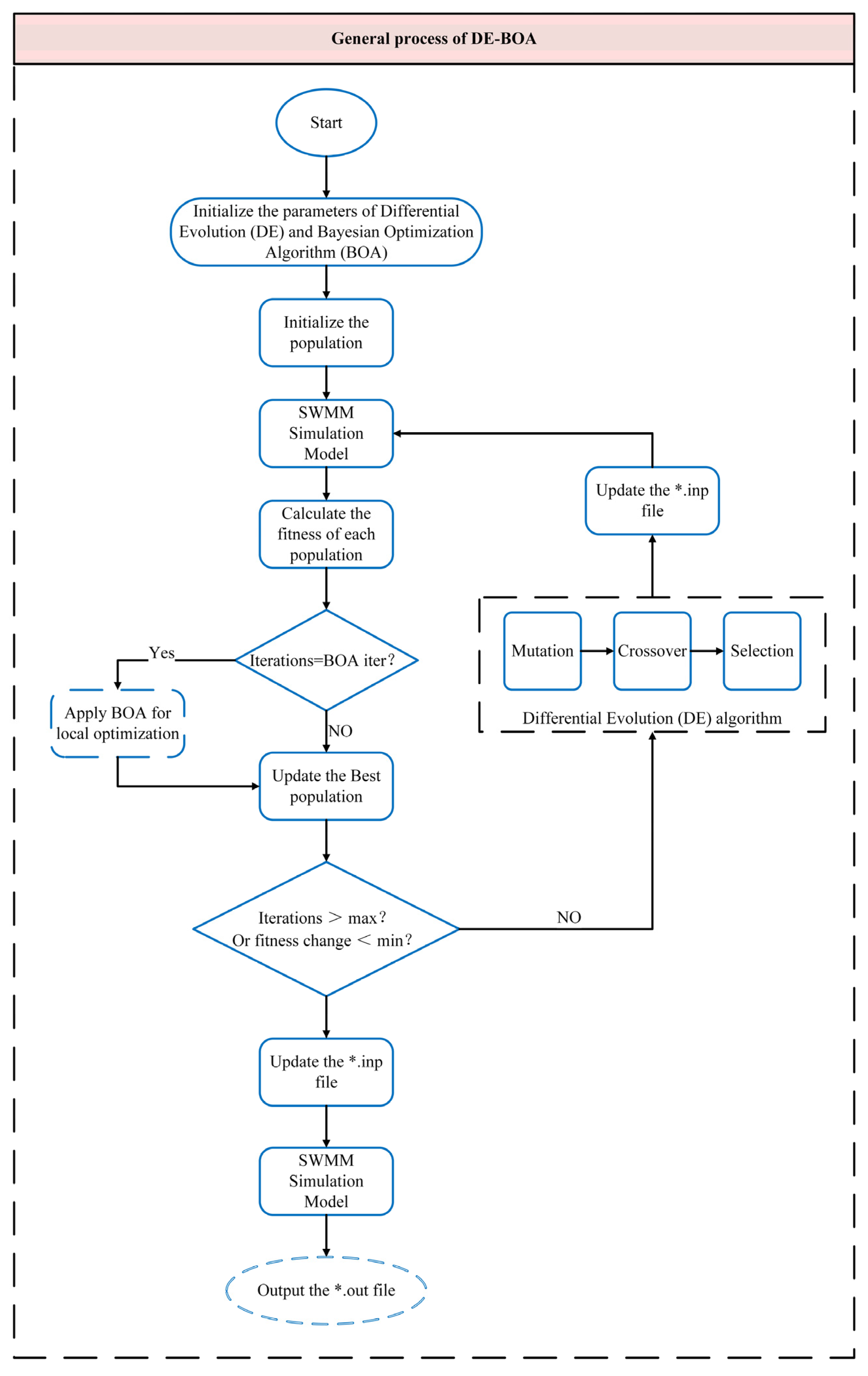
Building upon the foundation of the DE algorithm, we introduce the Gaussian process regression model from the BOA algorithm. This model captures the posterior distribution of the target function based on existing sample points. Using the collection function to guide the selection of the following sampling points, we combine the global search capability of the DE algorithm with the local search capability of the BOA algorithm. This hybrid optimization approach prevents the parameters from becoming trapped in local optima during the calibration process, so it achieves a high-precision parameter estimation for the SWMM model. Please refer to Figure 1 for the detailed algorithmic structure.
(2)
Using an adaptive weight allocation strategy, we tailor the distribution proportions of the DE algorithm and BOA algorithm, based on the balance between the constraints and the objective function of each specific SWMM model. During the initial stages of optimization, when the initial population exhibits good dispersion, we leverage the randomness of the initial population by assigning higher weights to the DE algorithm. By invoking the DE algorithm multiple times in the early phases, we enhance the exploration for the global optimum. However, as the optimization progresses, to avoid falling into local optima, we dynamically adjust the weights and increase the frequency of utilizing the BOA algorithm. Leveraging the characteristics of the BOA algorithm, which consider a more significant amount of historical data, we enhance the precision of SWMM model calibration and more thoroughly explore the global optimum. Please refer to Figure 2 for the detailed algorithmic flow.

2.4. Case Study

2.4.1. Overview of the Study Area

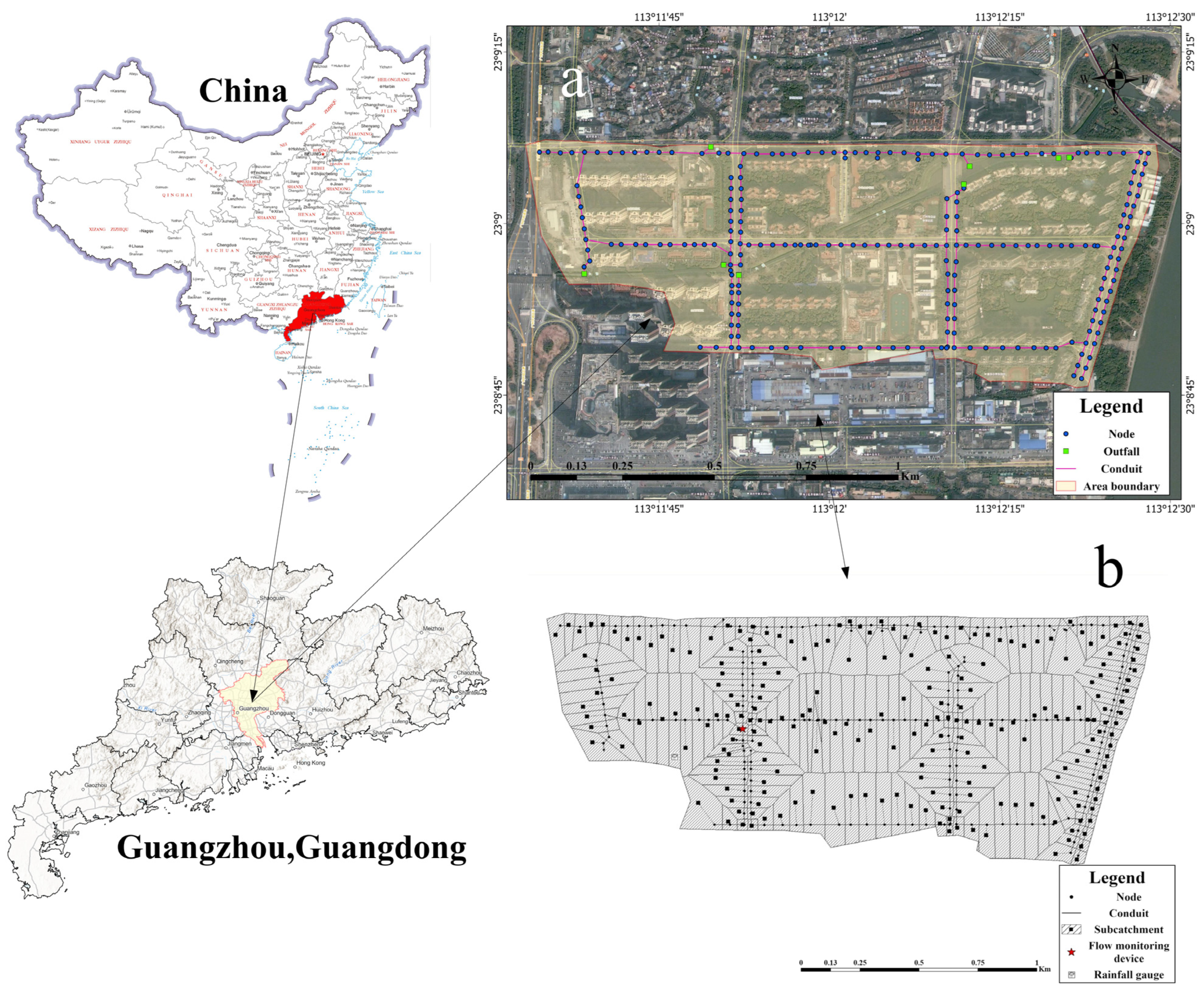
The present study selects an urban drainage sub-basin in Jinshazhou, Guangzhou, China, as the research case. The area of this sub-basin is 0.82 km2, and its location is illustrated in Figure 3a. Water systems, green spaces, and buildings intertwine in a mosaic-like distribution within the region, while primary and secondary roads crisscross, which creates a diverse urban land structure. Among them, impervious surfaces cover an area of 0.3 km2, which accounts for 36.6%, while pervious surfaces cover an area of 0.52 km2, which accounts for 63.4% (the land use types are depicted in Figure 4).
An urban stormwater runoff model was constructed based on the network data, land use types within the study area, and observed hydro-meteorological data. This SWMM model comprises 226 sub-catchments, 237 conduits, 226 nodes, and 8 outfalls, as depicted in Figure 3b. The rainfall and runoff data recorded by the rainfall gauge and flow monitoring device in Jinshazhou were utilized as the foundation for the precipitation and runoff analysis in this study.

2.4.2. Analysis of Rainfall Events

This study collected independent rainfall events from April to August 2022. To conduct statistical analysis on these events, a daily interval was used to distinguish between them. Since rainfall events with small total amounts and longer durations have minimal impact on the stormwater network facilities in the study area, as input conditions, the SWMM model for the study area only utilized rainfall events with total precipitation exceeding 10 mm within 24 h. Table 1 lists the rainfall events.
By conducting statistical analysis on 20 rainfall events, we classified the rainfall intensity levels of these events based on the classification standards issued by the China Meteorological Administration, i.e., rainfall between 10 and 24.9 mm in 24 h is regarded as moderate rainfall, rainfall between 25.0 and 49.9 mm in 24 h is regarded as heavy rainfall, and rainfall between 50.0 and 99.9 mm in 24 h is regarded as torrential rainfall. Among them, moderate, heavy, and torrential rain accounted for 25, 65, and 10% of the total rainfall events, respectively.
Using the classification criteria proposed by Yin et al. [30], which are suitable for Guangzhou City, we classified the rainfall characteristics of the 20 rainfall events based on seven types of heavy rainfall patterns. Table 2 presents the results. The analysis reveals that the selected independent rainfall events of this study encompass all commonly observed rainfall patterns in Guangzhou City, which are predominately single-peak heavy rainfall.

2.4.3. SWMM Model Parameters

In the SWMM model, parameters are typically classified into two types: those that can be directly measured through field surveys, and those that lack a precise physical definition, which makes them challenging to directly obtain. The latter type is usually estimated based on empirical ranges, which require the identification of sensitive parameters that significantly impact the model to improve the efficiency of calibration [31].
In this paper, the improved Morris screening method [31,32,33] is selected for sensitivity analysis, i.e., the idea of the control variable method is adopted to change the value of a parameter in a fixed step to affect the simulation results, under the condition of ensuring that the other parameters remain unchanged, and the average rate of change of the model results is taken as the sensitivity value of the parameter, which is calculated using the following formulas:
S = i = 1 n Y i + 1 Y i / Y 0 P i + 1 P i / 100 / n
where S is the sensitivity value; Y i is the output value of the ith run of the model; Y i + 1 is the output value of the i+1 th run of the model; Y 0 is the baseline output value of the model; P i is the percentage change in the parameter value of the ith model run relative to the calibrated parameter value; P i + 1 is the percentage change in the parameter value of the i+1 st model run relative to the calibrated parameter value; and n is the number of model runs.
When the value of S is less than 0.05, the parameter is insensitive. If the value of S is between 0.05 and 0.2, the parameter is moderately sensitive. If the value of S is between 0.2 and 1.0, the parameter is considered sensitive. A value of S greater than 1.0 indicates that the parameter is very sensitive. In this paper, the initial parameter value is changed in fixed steps of 10%, and the results of increasing its value by −25%, −15%, −5%, 5%, 15%, and 25% are obtained to calculate the sensitivity value of the parameter to total runoff, flood flow, and the peak present time, and the average value of S ¯ is taken as the main index for sensitivity analysis.
The results of the parameter sensitivity analysis are shown in Table 3, and the range of parameter values is derived from a combination of local engineering experience values and the SWMM User’s Manual.

2.4.4. SWMM Optimization Calculation

1.
Formulate the objective function
Given the significance of the peak flow values and peak occurrence time in urban flood disasters, this study is founded upon minimizing disparities in peak values and peak occurrence times. By integrating the Nash–Sutcliffe Efficiency (NSE), a multi-objective function is established to conduct a fitting analysis of the observed rainfall data and simulated results.
n u m 0 = i = 1 n I ( Q o , t Q p , t > P d t )
where n is the number of peaks, Q o , t is the observed flow at the ‘t’-th time step, Q p , t is the simulated flow at the ‘t’-th time step, and I is the indicator function. The indicator function takes the value of 1 when the absolute difference between Q o , t and Q p , t exceeds the tolerance for peak differences P d t , and 0 otherwise.
n u m 1 = i = 1 n I ( T o , t T p , t > T d t )
where T o , t is the peak occurrence time of the observed flow at the ‘t’-th time step, T p , t is the peak occurrence time of the simulated flow at the ‘t’-th time step, and I is the indicator function. The indicator function takes the value of 1 when the absolute difference between T o , t and T p , t exceeds the tolerance for peak differences T d t , and 0 otherwise.
N S E = 1 t = 1 T ( Q o , t Q p , t ) 2 t = 1 T ( Q o , t Q o , m ) 2  
where T is the length of the time series, Q o , m is the mean of the observed flow, and an NSE value closer to 1 indicates a more favorable calibration outcome of the model.
By combining Equations (7)–(9), we formulate a multi-objective function:
F = n u m 0 + n u m 1 × P + N S E
where P is a penalty factor to penalize the larger variance values that occur in the peak and peak present time.
2.
Simulation procedure
(1)
The SWMM model of the study area was simulated using the Horton infiltration model and the dynamic wave method. Four rainfall events (R3, R4, R7, and R13) were set aside for subsequent model validation, while the remaining 16 rainfall events were utilized as input conditions to calibrate the model parameters.
(2)
The population was initialized and the fundamental parameters of the DE-BOA algorithm were set, based on the experience of multiple iterations of trial and error in the previous sensitivity analysis: population size = 20; mutation factor = 0.8; crossover factor = 0.7; maximum iteration count = 100. Bayesian iteration factors were chosen as 5 and 2, respectively. Batch import and export of SWMM parameters was implemented using the Python language.
(3)
Three solutions were randomly selected from the initial population and trial individuals were generated using the mutation and crossover formulas. The Python language was utilized to invoke the SWMM calculation engine for simulation computation and to obtain simulated water depths at the monitoring locations.
(4)
The *.out file generated by the SWMM simulation was retrieved; the objective function values were calculated after simulation; a greedy selection strategy was employed; and the optimal value was selected as the calibrated parameter value. The *.inp file was modified to serve as the input file for the next round of SWMM simulation.
(5)
At the early stage of the algorithm, the BOA algorithm was applied every five generations based on the optimal value to locally optimize it. As the algorithm progressed, an adaptive strategy to increase the proportion of the BOA algorithm was used and the influence factor of the optimal historical value on the computation was adjusted. Multiple rounds of local optimization were performed based on the optimal value and a greedy selection strategy was applied to the results.
(6)
The calibrated *.inp file was generated as output.
3.
Evaluation criteria
R M S E = 1 T t = 1 T ( Q o , t Q p , t ) 2
where R M S E denotes the Root Mean Square Error, which is used to gauge the deviation between simulated flow and measured flow. A small value signifies a minor simulation error.
R 2 = t = 1 T Q p ,   t Q p ,   m Q o ,   t Q o ,   m 2 t = 1 T ( Q p ,   t Q p ,   m ) 2 t = 1 T ( Q o ,   t Q o ,   m ) 2
where R 2 is the coefficient of determination to assess the degree of fit and modeling capability of the algorithm. A higher value indicates a greater explanatory power of the independent variable on the dependent variable. Q p , t is the mean of the measured flow.
P E = Q p p Q o p Q o p
where P E is the peak relative error, which serves as a measure of the algorithm’s deviation in extreme situations. A smaller value signifies better simulation performance. Q p p and Q o p are the peak values of the simulated flow and measured flow, respectively.

3. Results and Discussion

3.1. Parameter Calibration Results

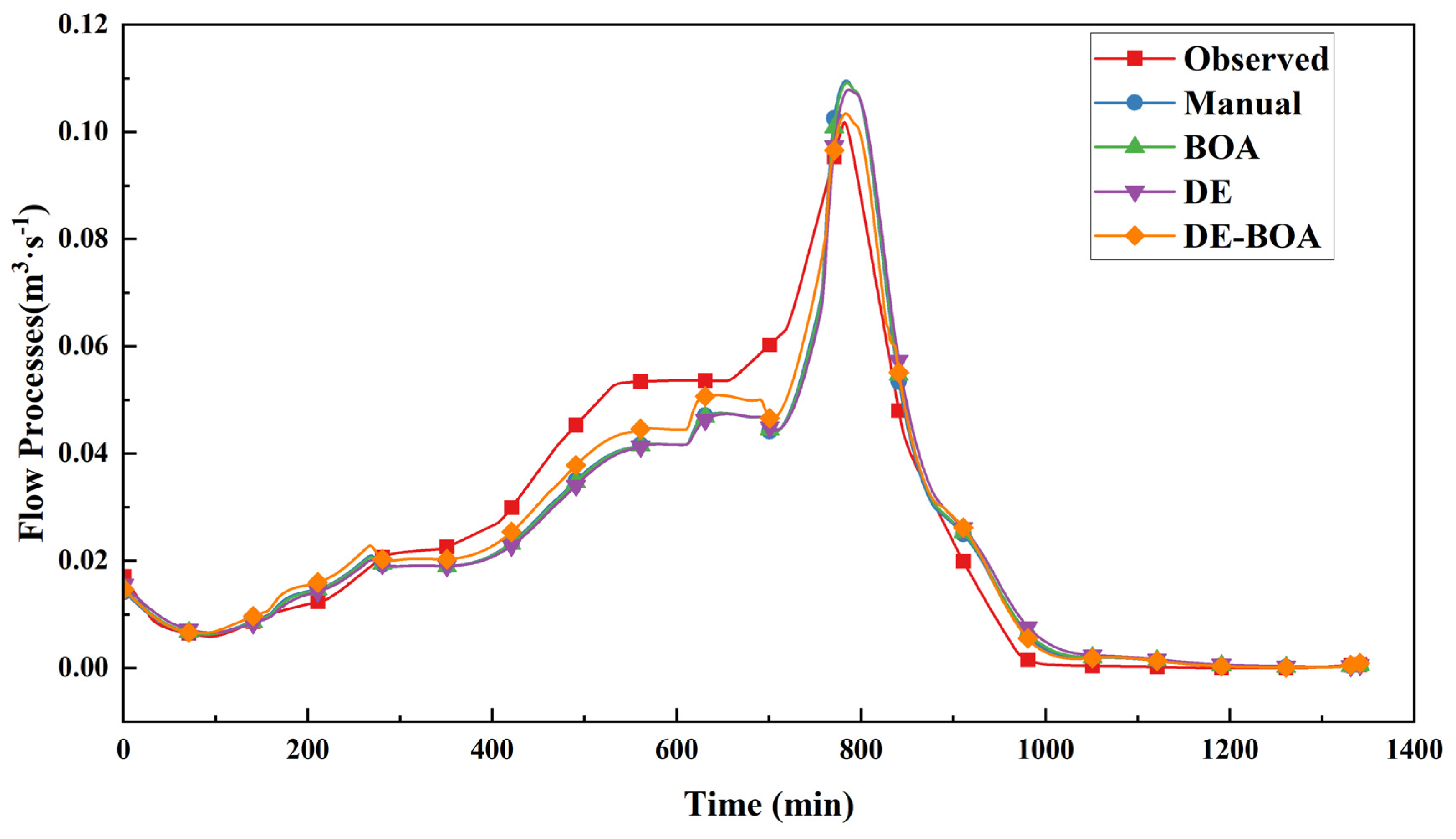
The model underwent parameter calibration using a selection of 16 rainfall events from Table 1. Taking R5 as an example, the calibrated flow process was compared to the observed flow process for the manual calibration, Bayesian optimization algorithm, differential evolution algorithm, and DE-BOA algorithm (Figure 5). With equal numbers of iterations, the objective function values were recorded to be 0.8846, 0.8704, 0.8795, and 0.9402. Compared to the other methods, the enhanced algorithm exhibited improvements of 6.29%, 8.02%, and 6.91%. Figure 5 shows that the DE-BOA algorithm outperformed the other approaches in flow prediction, since its peak flow and curve trends are more closely aligned with the observed flow.
Furthermore, different calibration methods were compared based on the evaluation metrics, as outlined in Table 4. The DE-BOA algorithm exhibits better RMSE, R2, and PE than the other methods to various degrees. The RMSE and R2 values indicate that, when calibrated using the DE-BOA algorithm, there is a good fit between observed and simulated flows. The PE value indicates that even in extreme circumstances, the DE-BOA algorithm maintains a commendable level of simulation performance.
The parameter rate setting speed of the algorithms is also one of the decisive factors affecting the application of intelligent algorithms. In this study, when comparing the speeds of DE, BOA, and DE-BOA algorithms to be the first to find the optimal objective function in 100 iterations (refer to Figure 6), the BOA algorithm achieved the optimal objective function value of 0.8704 in the 20th iteration, the DE algorithm achieved the optimal objective function value of 0.8795 in the 26th iteration, and the DE-BOA algorithm achieved the optimal objective function value of 0.9402 in the 13th iteration. This shows that the DE-BOA algorithm is not only faster but also more accurate in SWMM parameterization.
Based on the computed objective function values from the 16 rainfall instances, distinct weights were assigned. These weights were employed to calculate the calibrated model parameters (refer to Table 5). In comparison to the parameters obtained through manual calibration, the integrated approach demonstrated enhanced precision and substantial variations in specific parameter values. The primary underlying factor is that manual calibration typically relies on a trial-and-error method, which focuses on single-parameter adjustments. Hence, it fails to account for the intricate interplay among multiple parameters and is subjected to pronounced subjective inclinations. In contrast, the DE-BOA algorithm leverages its algorithmic traits to perform comprehensive global exploration and meticulous local refinement, thus enabling the search for optimal values within the vector solution space, which encompasses all calibrated parameters.

3.2. Model Verification

To assess the accuracy and credibility of the calibrated model, we input the four rainfall events selected for validation (refer to Table 6) into the SWMM model. These events (R3, R4, R7, and R13) include various rainfall intensities and types within the study area, which enables an exploration of the impact of different rainfall event types on the model’s simulation.
In Figure 7, the comparison between calibrated and measured flow processes of the four rainfall events reveals that all NSE values of the model exceed 0.85. This result signifies a remarkable concordance between simulated and observed flow processes, which satisfies the application requirements of the SWMM model. R4 and R13 exhibit the highest NSE values of 0.9317 and 0.9306, respectively, which can be attributed to their correlation with the rainfall dynamics. When multiple rainfall peaks and substantial precipitation occur, the predictive accuracy of the model more closely aligns with the actual observed values. Thus, the DE-BOA algorithm exhibits greater adaptability when handling rainfall data characterized by multiple peaks and a significant rainfall volume.

4. Conclusions

The present study proposed a calibration method for the SWMM model based on the DE-BOA algorithm. To demonstrate the feasibility and applicability of the DE-BOA algorithm, a case study was conducted in a drainage sub-catchment in Jinshazhou, Guangzhou. The rainfall events in the area were analyzed for their characteristics, and a multi-objective function was constructed to evaluate the algorithm’s performance. The comparison of the simulated flow process of the algorithm with the rest of the rate determination methods shows that the DE-BOA algorithm performs well on the evaluation metrics RMSE, R2, and PE, which reach 0.0052, 0.9644, and 0.0161, respectively, and the objective function value is improved by 6.29%, 8.02%, and 6.91% compared with the rest of the methods, and meanwhile, in terms of the rate setting rate and the rate setting process, the DE-BOA algorithm also shows obvious advantages. The algorithmic model enables the automatic parameter calibration of SWMM with high accuracy and at a faster rate, which effectively improves the modeling efficiency. This result provides valuable insights for the dynamic updating of model parameters and improves the performance and accuracy of modeling on intelligent water management platforms.
The calibration validation of the model demonstrates a significant improvement in the calibration effectiveness of the DE-BOA algorithm for rainfall events with multiple peaks and substantial precipitation. It must be admitted that this study has some limitations, because, due to the confidentiality of the geographic information data, we only obtained a limited number of sample data, which may affect the generalization of the results. Therefore, the question of how to further improve the algorithm rate accuracy, as well as the generalizability, will be considered in future research.

Author Contributions

Conceptualization, J.L. and J.G.; methodology, J.L. and J.G.; investigation, Y.L. and R.Z.; data curation, J.L.; writing—original draft preparation, J.G.; writing—review and editing, J.L. and X.L.; supervision, J.L. All authors have read and agreed to the published version of the manuscript.

Funding

This study was supported by the National Key R&D Program of China (2022YFC3002704) and the Natural Science Foundation of Hubei Province of China (2022CFB042).

Data Availability Statement

All data, models, and code that support the findings of this study are available from the corresponding author upon reasonable request.

Acknowledgments

We are grateful to the editors and anonymous reviewers for their thoughtful comments.

Conflicts of Interest

The authors declare no conflict of interest.

References

  1. Hossain, S.; Hewa, G.A.; Wella-Hewage, S. A Comparison of Continuous and Event-Based Rainfall–Runoff (RR) Modelling Using EPA-SWMM. Water 2019, 11, 611. [Google Scholar] [CrossRef]
  2. Tsihrintzis, V.A.; Hamid, R. Runoff Quality Prediction from Small Urban Catchments Using SWMM. Hydrol. Process. 1998, 12, 311–329. [Google Scholar] [CrossRef]
  3. Jang, S.; Cho, M.; Yoon, J.; Yoon, Y.; Kim, S.; Kim, G.; Kim, L.; Aksoy, H. Using SWMM as a Tool for Hydrologic Impact Assessment. Desalination 2007, 212, 344–356. [Google Scholar] [CrossRef]
  4. Yao, L.; Chen, L.; Wei, W. Assessing the Effectiveness of Imperviousness on Stormwater Runoff in Micro Urban Catchments by Model Simulation. Hydrol. Process. 2016, 30, 1836–1848. [Google Scholar] [CrossRef]
  5. Guan, M.; Sillanpää, N.; Koivusalo, H. Storm Runoff Response to Rainfall Pattern, Magnitude and Urbanization in a Developing Urban Catchment. Hydrol. Process. 2016, 30, 543–557. [Google Scholar] [CrossRef]
  6. Sun, N.; Hong, B.; Hall, M. Assessment of the SWMM Model Uncertainties within the Generalized Likelihood Uncertainty Estimation (GLUE) Framework for a High-Resolution Urban Sewershed. Hydrol. Process. 2014, 28, 3018–3034. [Google Scholar] [CrossRef]
  7. Zaghloul, N.A. Sensitivity Analysis of the SWMM Runoff-Transport Parameters and the Effects of Catchment Discretisation. Adv. Water Resour. 1983, 6, 214–223. [Google Scholar] [CrossRef]
  8. Barco, J.; Wong, K.M.; Stenstrom, M.K. Automatic Calibration of the U.S. EPA SWMM Model for a Large Urban Catchment. J. Hydraul. Eng. 2008, 134, 466–474. [Google Scholar] [CrossRef]
  9. Del Giudice, G.; Padulano, R. Sensitivity Analysis and Calibration of a Rainfall-Runoff Model with the Combined Use of EPA-SWMM and Genetic Algorithm. Acta Geophys. 2016, 64, 1755–1778. [Google Scholar] [CrossRef]
  10. Kim, S.W.; Kwon, S.H.; Jung, D. Development of a Multiobjective Automatic Parameter-Calibration Framework for Urban Drainage Systems. Sustainability 2022, 14, 8350. [Google Scholar] [CrossRef]
  11. Tscheikner-Gratl, F.; Zeisl, P.; Kinzel, C.; Leimgruber, J.; Ertl, T.; Rauch, W.; Kleidorfer, M. Lost in Calibration: Why People Still Do Not Calibrate Their Models, and Why They Still Should—A Case Study from Urban Drainage Modelling. Water Sci. Technol. 2016, 74, 2337–2348. [Google Scholar] [CrossRef]
  12. Gulbaz, S.; Kazezyilmaz-Alhan, C.M. Calibrated Hydrodynamic Model for Sazlidere Watershed in Istanbul and Investigation of Urbanization Effects. J. Hydrol. Eng. 2013, 18, 75–84. [Google Scholar] [CrossRef]
  13. Jin, X.; Jiang, Y.; Wu, W.; Jin, J. Automatic Calibration of SWMM Model with Adaptive Genetic Algorithm. In Proceedings of the 2011 International Symposium on Water Resource and Environmental Protection, Xi’an, China, 20–22 May 2011; Volume 2, pp. 891–895. [Google Scholar]
  14. Wan, B.; James, W. SWMM Calibration Using Genetic Algorithms. In Global Solutions for Urban Drainage; American Society of Civil Engineers: Reston, VA, USA, 2012; pp. 1–14. [Google Scholar] [CrossRef]
  15. Gao, X.; Yang, Z.; Han, D.; Huang, G.; Zhu, Q. A Framework for Automatic Calibration of SWMM Considering Input Uncertainty. Hydrol. Earth Syst. Sci. Discuss. 2020, 1–25. [Google Scholar] [CrossRef]
  16. Perin, R.; Trigatti, M.; Nicolini, M.; Campolo, M.; Goi, D. Automated Calibration of the EPA-SWMM Model for a Small Suburban Catchment Using PEST: A Case Study. Env. Monit Assess 2020, 192, 374. [Google Scholar] [CrossRef]
  17. Shahed Behrouz, M.; Zhu, Z.; Matott, L.S.; Rabideau, A.J. A New Tool for Automatic Calibration of the Storm Water Management Model (SWMM). J. Hydrol. 2020, 581, 124436. [Google Scholar] [CrossRef]
  18. Azad, A.; Manoochehri, M.; Kashi, H.; Farzin, S.; Karami, H.; Nourani, V.; Shiri, J. Comparative Evaluation of Intelligent Algorithms to Improve Adaptive Neuro-Fuzzy Inference System Performance in Precipitation Modelling. J. Hydrol. 2019, 571, 214–224. [Google Scholar] [CrossRef]
  19. Farzin, S.; Valikhan Anaraki, M. Optimal Construction of an Open Channel by Considering Different Conditions and Uncertainty: Application of Evolutionary Methods. Eng. Optim. 2021, 53, 1173–1191. [Google Scholar] [CrossRef]
  20. Sambito, M.; Freni, G. Strategies for Improving Optimal Positioning of Quality Sensors in Urban Drainage Systems for Non-Conservative Contaminants. Water 2021, 13, 934. [Google Scholar] [CrossRef]
  21. Storn, R.; Price, K. Differential Evolution: A Simple and Efficient Adaptive Scheme for Global Optimization Over Continuous Spaces. J. Glob. Optim. 1995, 23, 1–15. [Google Scholar]
  22. Bai, Y.; Lu, W.; Li, J.; Chang, Z.; Wang, H. Groundwater Contamination Source Identification Using Improved Differential Evolution Markov Chain Algorithm. Env. Sci Pollut Res 2022, 29, 19679–19692. [Google Scholar] [CrossRef]
  23. Smith, T.J.; Marshall, L.A. Bayesian Methods in Hydrologic Modeling: A Study of Recent Advancements in Markov Chain Monte Carlo Techniques. Water Resour. Res. 2008, 44, 1–9. [Google Scholar] [CrossRef]
  24. McDonnell, B.E.; Ratliff, K.; Tryby, M.E.; Wu, J.J.X.; Mullapudi, A. PySWMM: The Python Interface to Stormwater Management Model (SWMM). J. Open Source Softw. 2020, 5, 2292. [Google Scholar] [CrossRef]
  25. Zhang, X.; Srinivasan, R.; Zhao, K.; Liew, M.V. Evaluation of Global Optimization Algorithms for Parameter Calibration of a Computationally Intensive Hydrologic Model. Hydrol. Process. 2009, 23, 430–441. [Google Scholar] [CrossRef]
  26. Brest, J.; Greiner, S.; Boskovic, B.; Mernik, M.; Zumer, V. Self-Adapting Control Parameters in Differential Evolution: A Comparative Study on Numerical Benchmark Problems. IEEE Trans. Evol. Comput. 2006, 10, 646–657. [Google Scholar] [CrossRef]
  27. Shao, Z.; Xu, L.; Chai, H.; Yost, S.A.; Zheng, Z.; Wu, Z.; He, Q. A Bayesian-SWMM Coupled Stochastic Model Developed to Reconstruct the Complete Profile of an Unknown Discharging Incidence in Sewer Networks. J. Environ. Manag. 2021, 297, 113211. [Google Scholar] [CrossRef]
  28. Muleta, M.K.; McMillan, J.; Amenu, G.G.; Burian, S.J. Bayesian Approach for Uncertainty Analysis of an Urban Storm Water Model and Its Application to a Heavily Urbanized Watershed. J. Hydrol. Eng. 2013, 18, 1360–1371. [Google Scholar] [CrossRef]
  29. Yazdi, J.; Yoo, D.G.; Kim, J.H. Comparative Study of Multi-Objective Evolutionary Algorithms for Hydraulic Rehabilitation of Urban Drainage Networks. Urban Water J. 2017, 14, 483–492. [Google Scholar] [CrossRef]
  30. Yin, L.; Chen, X.; Chen, Z.; Shuai, W.; Zhang, M.; Liu, H. Study on Storm Pattern of Typical Rainfall Station in Guangzhou. J. Water Resour. Res. 2013, 2, 409. [Google Scholar] [CrossRef]
  31. Zhong, B.; Wang, Z.; Yang, H.; Xu, H.; Gao, M.; Liang, Q. Parameter Optimization of SWMM Model Using Integrated Morris and GLUE Methods. Water 2023, 15, 149. [Google Scholar] [CrossRef]
  32. Lenhart, T.; Eckhardt, K.; Fohrer, N.; Frede, H.-G. Comparison of Two Different Approaches of Sensitivity Analysis. Phys. Chem. Earth Parts A/B/C 2002, 27, 645–654. [Google Scholar] [CrossRef]
  33. Morris, M.D. Factorial Sampling Plans for Preliminary Computational Experiments. Technometrics 1991, 33, 161–174. [Google Scholar] [CrossRef]
Figure 1. Structure of the Differential Evolution and Bayesian Optimization Algorithm.
Water 15 03582 g001
Figure 2. Flowchart of the Differential Evolution and Bayesian Optimization Algorithm.
Water 15 03582 g002
Figure 3. Location and model structure of the study area: (a) geographical location of the study area; (b) SWMM pipe network mode.
Water 15 03582 g003
Figure 4. Land use types.
Water 15 03582 g004
Figure 5. Comparison of flow processes for different rate determination methods.
Water 15 03582 g005
Figure 6. Comparison of rate speeds for different rate determination methods.
Water 15 03582 g006
Figure 7. Verification of model calibration results.
Water 15 03582 g007
Table 1. The statistics of rainfall events in the study area.
IDStart TimeEnd TimeTotal Rainfall
(mm)
Rainfall Duration
(h)
Rainfall Scale
R130 April 2022 16:001 May 2022 0:0014.028 hModerate rain
R21 May 2022 4:101 May 2022 20:2036.0216.17 hHeavy rain
R37 May 2022 7:407 May 2022 18:2019.8710.67 hModerate rain
R410 May 2022 1:5011 May 2022 0:0048.4722.17 hHeavy rain
R511 May 2022 0:0012 May 2022 0:0081.2624 hRainstorm
R612 May 2022 10:3013 May 2022 20:2024.659.84 hModerate rain
R713 May 2022 0:0014 May 2022 0:0080.7524 hRainstorm
R821 May 2022 13:4022 May 2022 0:0026.9111.67 hHeavy rain
R96 June 2022 10:106 June 2022 22:5026.7312.67 hHeavy rain
R107 June 2022 9:307 June 2022 19:1043.709.67 hHeavy rain
R119 June 2022 7:2010 June 2022 12:3032.785.17 hHeavy rain
R1212 June 2022 8:0012 June 2022 18:3025.1810.5 hHeavy rain
R1313 June 2022 1:4013 June 2022 16:5035.0915.17 hHeavy rain
R1415 June 2022 8:2015 June 2022 20:5034.6412.5 hHeavy rain
R1517 June 2022 4:3017 June 2022 17:1032.3012.67 hHeavy rain
R1619 June 2022 1:2019 June 2022 14:2023.7813 hModerate rain
R172 July 2022 0:002 July 2022 22:4046.7322.67 hHeavy rain
R186 July 2022 11:406 July 2022 19:4030.948 hHeavy rain
R193 August 2022 15:103 August 2022 18:4023.003.5 hModerate rain
R2010 August 2022 8:0010 August 2022 16:3027.098.5 hHeavy rain
Table 2. Rainfall event rain type.
Rainfall PatternFrequency (Times)Proportion
Single peak ahead (type I)15%
Single peak back (type II)525%
Single peak centered (type III)525%
Uniform distribution (type IV)15%
Distribution before and after bimodal (type V)15%
Bimodal distribution (type VI)420%
Bimodal mid-post distribution (type VII)315%
Table 3. Parameters to be determined and value ranges.
Calibration ParametersParameter Meaning S ¯ Ranges
N-ImpervManning coefficient of impermeable area0.0695670.01~0.05
N-PervManning coefficient of permeable area0.0547670.05~0.4
S-Imperv/mmDepression volume in impermeable area0.0541330.2~10
S-Perv/mmDepression storage volume in permeable area0.08792~20
MinRate/(mm·h−1)Minimum infiltration rate0.0516331~20
MaxRate/(mm·h−1)Maximum infiltration rate0.05316720~100
Decay/h−1Permeation attenuation coefficient0.0727672~7
Table 4. Evaluation metrics for simulating results using different calibration methods.
MethodBOADEManualDE-BOA
RMSE0.00710.00750.00700.0052
R20.93000.92160.93390.9644
PE0.07270.06050.07680.0161
Table 5. SWMM calibration results.
ParametersInitial Empirical ValueRate Value
Manual
Calibration
DE-BOA
Calibration
N-Imperv0.0120.010.01
N-Perv0.20.40.3528
S-Imperv/mm0.450.20.2
S-Perv/mm22017.3671
MinRate/(mm·h−1)12.71811.0311
MaxRate/(mm·h−1)2009049.8109
Decay/h−1432.9728
Table 6. Rainfall events of the validation set.
IDTotal Rainfall
(mm)
Rainfall Duration
(h)
Rainfall ScaleRainfall Pattern
R319.8710.67 hModerate rainIV
R448.4722.17 hHeavy rainVII
R780.7524 hRainstormII
R1335.0915.17 hHeavy rainV
Disclaimer/Publisher’s Note: The statements, opinions and data contained in all publications are solely those of the individual author(s) and contributor(s) and not of MDPI and/or the editor(s). MDPI and/or the editor(s) disclaim responsibility for any injury to people or property resulting from any ideas, methods, instructions or products referred to in the content.