The Driving Effects of the Total Water Use Evolution in China from 1965 to 2019

Abstract

To understand the influence mechanism of the total water use evolution in a certain region more deeply, it is necessary to accurately identify the driving effects of the total water use evolution, and quantitatively analyze the influence of the driving effects on the total water use evolution. In this research, we studied the driving effects of the total water use evolution in China from the perspective of multi-year long time-series in the whole country for the first time. Through the logarithmic mean Divisia index (LMDI) decomposition method, we constructed an LMDI decomposition model for the regional total water use evolution, and decomposed the total water use evolution in China and its five stages from 1965 to 2019 into the water use intensity effect (WUIE), sector proportion effect (SPE), per capita total economy effect (PCTEE), and total population effect (TPE). We also considered the driving effects of the total water use evolution when the population or economic proportion changed in the six major districts in China for the first time. Based on the LMDI decomposition method, we separately added the district population proportion variable and the district economic proportion variable to contrast a logarithmic mean Disivia index-population (LMDI-P) decomposition model and a logarithmic mean Divisia index-economic (LMDI-E) decomposition model for the regional total water use evolution. Compared with the LMDI decomposition model, the district population proportion effect (DPPE) and the district economic proportion effect (DEPE) were separately added. We calculated the value and proportion of the driving effects of the total water use evolution in China and analyzed their influence mechanisms. Our findings provide better decision-making reference for water resource planning and management in China. The results show the following: (1) According to the overall situation from 1965 to 2019, the prohibitive role played by the PCTEE (total 22,263.79 × 10⁸ m³) and the TPE (total 2945.38 × 10⁸ m³) with respect to the total water use increasing in China offset the inhibitive role played by the WUIE (total −16,094.31 × 10⁸ m³) and the SPE (total −5930.02 × 10⁸ m³) with respect to the total water use increasing in China; (2) According to the overall situation from 1965 to 2019, both the DPPE and DEPE had heterogeneity in the total water use evolution in the six major districts in China. The DPPE played a prohibitive role in the three population inflow districts (Southeast China, Central South China, and Northwest China) with respect to the total water use increasing (total 291.09 × 10⁸ m³), and an inhibitive role in the other three population outflow districts (North China, Central South China, and Southwest China) with respect to the total water use increasing (total −207.78 × 10⁸ m³). The DEPE played a prohibitive role in the three economically developed districts (North China, Southeast China, and Central South China) with respect to the total water use increasing (total 428.26 × 10⁸ m³), and an inhibitive role in the other three economically underdeveloped districts (Northeast China, Southwest China, and Northwest China) with respect to the total water use increasing (total −477.74 × 10⁸ m³).

1. Introduction

In recent years, water scarcity has become a major bottleneck constraining sustainable socio-economic development due to the uncontrolled exploitation of water resourses by human beings and changes in the climate [1,2]. In response to this problem, many countries have begun to pay attention to the prediction of future water demand, which is used to guide water resource planning and management to meet the challenges of sustainable water resource utilization [3,4]. In the past, it was traditionally recognized that population growth, economic growth, improved living standards, and the resulting changes in lifestyles tended to increase water demand and that total water use would continue to grow with socio-economic development [5,6]. However, since the 1980s, the total water use in many developed countries and districts worldwide has tended to be stable or even in decline, which has increased scholars’ attention and exploration regarding the rule of total water use growth [7,8].

China is one of the most water-scarce countries in the world, and water resource shortages will seriously hinder the sustainable development of the country [9]. In order to solve the problem of water resource shortages and improve water resource utilization efficiency, the Chinese government has adopted a series of water-saving policies and measures, including investing in water conservancy facilities and implementing water-saving technology reforms in different sectors [10]. The total water use in China increased from 2836.58 × 10⁸ m³ in 1965 to 6183.53 × 10⁸ m³ in 2013, then decreased to 6021.42 × 10⁸ m³ in 2019, representing a total increase of 3184.84 × 10⁸ m³, and a process of rapid rise to slow decline. Therefore, it can be seen that China’s water-saving policy has achieved some positive results [11].

Many scholars at home and abroad have studied the influence of economic growth on total water use evolution [12,13]. Some scholars have introduced relevant methods in the field of resource and environmental research to address the problem, such as “the environmental Kuznets curve” and “decoupling theory”, but the total water use evolution is the result of a combination of many factors, not just economic growth [14,15]. Therefore, to understand the influence mechanisms of the total water use evolution in a certain region more deeply, it is necessary to accurately identify the driving effects of the total water use evolution, and quantitatively analyze the influence of the driving effects on the total water use evolution. This also has practical significance for effectively coping with water resource shortages in China [16].

Scholars at home and abroad have also studied the driving effects of the total water use evolution [17]. In recent years, the index decomposition analysis method has been widely applied to the problem of the total water use evolution driving effect decomposition [18]. On this basis, Ang et al. proposed the Divisia index decomposition method and constructed the logarithmic mean Divisia index (LMDI) decomposition model, which is considered to be the optimal decomposition model [19,20,21]. There are many existing studies on the regional total water use evolution driving effect investigated through the LMDI decomposition model. Yang and Chen summarized the driving factors of water use change in Guangdong as population, wealth, structure, and technology [22]. Du et al. found that agricultural water use efficiency and population had a positive effect on water use change in Ningxia, while water resource stress, structure, and endowment had a negative effect on water use change in Ningxia [23]. However, there were few studies on the total water use evolution driving effect in China from the perspective of multi-year long time-series in the whole country, and this could not comprehensively explain the influence mechanism of the total water use evolution in China. There were also few studies considering the driving effects of the total water use evolution in China when the population or economic proportion changed in the six major districts in China, and this could not comprehensively reflect the actual water demand in these districts.

The main contributions of this paper are as follows: (1) We studied the driving effects of the total water use evolution in China from the perspective of multi-year long time-series in the whole country for the first time; this could comprehensively explain the influence mechanism of the total water use evolution in China and provide a complete research example for scholars studying related fields in other countries. Through the LMDI decomposition method, we constructed an LMDI decomposition model for the regional total water use evolution, and decomposed the total water use evolution in China and its five stages from 1965 to 2019 into the water use intensity effect (WUIE), sector proportion effect (SPE), per capita total economy effect (PCTEE), and total population effect (TPE). We calculated the value and proportion of the driving effects of the total water use evolution in China and analyzed their influence mechanisms. Our findings provide better decision-making reference for water resource planning and management in China; (2) We also considered the driving effects of the total water use evolution when the population or economic proportion changed in the six major districts in China for the first time, this could comprehensively reflect the actual water demand in these districts. Based on the LMDI decomposition method, we separately added the district population proportion variable and the district economic proportion variable to contrast a logarithmic mean Disivia index-population (LMDI-P) decomposition model and a logarithmic mean Divisia index-economic (LMDI-E) decomposition model for the regional total water use evolution. Compared with the LMDI decomposition model, the district population proportion effect (DPPE) and the district economic proportion effect (DEPE) were separately added. We calculated the value and proportion of the two driving effects of the total water use evolution in the six major districts in China, and analyzed their influence mechanisms.

The rest of this paper is organized as follows: In Section 2, we introduce the materials and methods, including data sources and study methods (the LMDI decomposition model, the LMDI-P decomposition model, and the LMDI-E decomposition model). In Section 3, we describe the results, including the driving effects of the total water use evolution in China from 1965 to 2019 and its five stages, the driving effects of the total water use evolution in the six major districts in China from 1965 to 2019 considering the district population proportion variable, and the driving effects of the total water use evolution in the six major districts in China from 1965 to 2019 considering the district economic proportion variable. In Section 4, we discuss the results, including analysis of the driving effects of the total water use evolution in China from 1965 to 2019 and its five stages, and analysis of the DPPE and DEPE of the total water use evolution in the six major districts in China from 1965 to 2019. In Section 5, we outline the conclusions and prospects.

2. Materials and Methods

2.1. Data Sources

The data used in this research included the total water use (including the agricultural, industrial, and other sector water use), the total population, and the gross domestic (regional) product (including the agricultural, industrial, and other sector added value) of China and its 31 provincial administrative districts (data missing for Hong Kong, Macao, and Taiwan) from 1965 to 2019. The total water use data from 1965 to 1996 were obtained from the National Long-term Water Use Dataset of China [24], and from 1997 to 2019 were obtained from the China Water Resources Bulletin [25]. Both the total population and the gross domestic (regional) product data from 1965 to 2008 were obtained from the China Compendium of Statistics 1949–2008 [26], and from 2009 to 2019 were obtained from the China Statistical Yearbook [27]. To eliminate the effect of price factors, the gross domestic (regional) product from 1965 to 2019 was uniformly converted into the comparable price for the year 1978 (1978 = 100). To better discuss the results, the data were segmented temporally and partitioned spatially [28] (Figure 1).

2.2. Study Methods

2.2.1. The LMDI Decomposition Model

The LMDI decomposition model is used to study the driving effects of the total water use evolution in a region at a certain period. The calculation formula is as follows:

$$W={\displaystyle \sum _{j=1}^n{W}_j}={\displaystyle \sum _{j=1}^n\frac{W_j}{V_j}\times \frac{V_j}{G}\times \frac{G}{P}\times P}={\displaystyle \sum _{j=1}^{n}In{t}_j}\times P_{V_j}\times P{C}_{GDP}\times P$$

(1)

Here, $W$ denotes the total water use in a region at a certain time, $W_j$ denotes the $j$th sector water use in a region at a certain time, $V_j$ denotes the $j$th sector added value in a region at a certain time, $G$ denotes the gross domestic product in a region at a certain time, $P$ denotes the total population in a region at a certain time, $In{t}_j$ = $\frac{W_j}{V_j}$ denotes the $j$th sector water use intensity in a region at a certain time, $P_{V_j}$ = $\frac{V_j}{G}$ denotes the proportion of the $j$th sector added value to the gross domestic product in a region at a certain time, and $P{C}_{GDP}$ = $\frac{G}{P}$ denotes the per capita gross domestic product in a region at a certain time.

We assume that at a certain period (from time $t_1$ to time $t_2$), the following formulae exist:

$$\Delta W=\Delta W_{In{t}_j}+\Delta W_{P_{V_j}}+\Delta W_{P{C}_{GDP}}+\Delta W_P$$

(2)

$$\Delta W_{In{t}_j}={\displaystyle \sum _{j=1}^n\frac{W_j{}^{t_2}-W_j{}^{t_1}}{\ln W_j{}^{t_2}-\ln W_j{}^{t_1}}}\ln \frac{In{t}_j{}^{t_2}}{In{t}_j{}^{t_1}}$$

(3)

$$\Delta W_{P_{V_j}}={\displaystyle \sum _{j=1}^n\frac{W_j{}^{t_2}-W_j{}^{t_1}}{\ln W_j{}^{t_2}-\ln W_j{}^{t_1}}}\ln \frac{P_{V_j}{}^{t_2}}{P_{V_j}{}^{t_1}}$$

(4)

$$\Delta W_{P{C}_{GDP}}=\frac{W^{t_2}-W^{t_1}}{\ln W^{t_2}-\ln W^{t_1}}\ln \frac{P{C}_{GDP}{}^{t_2}}{P{C}_{GDP}{}^{t_1}}$$

(5)

$$\Delta W_P=\frac{W^{t_2}-W^{t_1}}{\ln W^{t_2}-\ln W^{t_1}}\ln \frac{P^{t_2}}{P^{t_1}}$$

(6)

Here, $\Delta W$ denotes the total water use variation (TWUV) in a region at a certain period; $\Delta W_{In{t}_j}$, $\Delta W_{P_{V_j}}$, $\Delta W_{P{C}_{GDP}}$, and $\Delta W_P$ separately denote the water use intensity effect (WUIE), sector proportion effect (SPE), per capita total economy effect (PCTEE), and total population effect (TPE), separately reflecting the influence of water use intensity, sector proportion, per capita total economy, and total population on the total water use evolution in a region at a certain period.

In this research, $t_1$, $t_2$∈{1965, 1966,…, 2019} ($t_2$ > $t_1$); $W$ denotes the total water use in China each year from 1965 to 2019; $W_j$ ($j$ = 1, 2, 3) separately denotes the agricultural, industrial, and other sector (including living and ecology) water use in China each year from 1965 to 2019; $V_j$ ($j$ = 1, 2, 3) separately denotes the agricultural, industrial, and other sector added value in China each year from 1965 to 2019; $G$ denotes the gross domestic product in China each year from 1965 to 2019; $P$ denotes the total population in China each year from 1965 to 2019; $In{t}_j$($j$ = 1, 2, 3) separately denotes the agricultural, industrial, and other sector water use intensity in China each year from 1965 to 2019; $P_{V_j}$ ($j$ =1, 2, 3) separately denotes the proportion of the agricultural, industrial, and other sector added value to the gross domestic product in China each year from 1965 to 2019; $P{C}_{GDP}$ denotes the per capita gross domestic product in China each year from 1965 to 2019; $\Delta W$ denotes the TWUV in China each annum (stage) from 1965 to 2019; $\Delta W_{In{t}_j}$ ($j$ = 1, 2, 3) separately denotes the agricultural water use intensity effect (AWUIE), industrial water use intensity effect (IWUIE), and other sector water use intensity effect (OWUIE) in China each annum (stage) from 1965 to 2019; $\Delta W_{P_{V_j}}$ ($j$ = 1, 2, 3) separately denotes the agricultural sector proportion effect (ASPE), industrial sector proportion effect (ISPE), and other sector proportion effect (OSPE) in China each annum (stage) from 1965 to 2019; $\Delta W_{P{C}_{GDP}}$ denotes the PCTEE in China each annum (stage) from 1965 to 2019; $\Delta W_P$ denotes the TPE in China each annum (stage) from 1965 to 2019.

2.2.2. The LMDI-P Decomposition Model

If a region consists of i districts, based on Formula (1), we can add the district population proportion variable $P_{P_i}$ to create the LMDI-P decomposition model. The calculation formula is as follows:

$$W_i={\displaystyle \sum _{i=1}^m{\displaystyle \sum _{j=1}^n{W}_{ij}}}={\displaystyle \sum _{i=1}^m{\displaystyle \sum _{j=1}^n\frac{W_{ij}}{V_{ij}}}}\times \frac{V_{ij}}{G_i}\times \frac{G_i}{P_i}\times \frac{P_i}{P}\times P={\displaystyle \sum _{i=1}^m{\displaystyle \sum _{j=1}^{n}In{t}_{ij}\times P_{V_{ij}}\times P{C}_{GRP}{}_{{}_i}\times P_{P_i}\times P}}$$

(7)

Here, $P_{P_i}$ = $\frac{P_i}{P}$ denotes the total population proportion of the $i$th district of a region to the region at a certain time.

We assume that at a certain period (from time $t_1$ to time $t_2$), the following formula exists:

$$\Delta W_i=\Delta W_{In{t}_{ij}}+\Delta W_{P_{V_{ij}}}+\Delta W_{P{C}_{GR{P}_i}}+\Delta W_{P_{P_i}}+\Delta W_{P_i}$$

(8)

$$\Delta W_{In{t}_{ij}}={\displaystyle \sum _{i=1}^m{\displaystyle \sum _{j=1}^n\frac{W_{ij}{}^{t_2}-W_{ij}{}^{t_1}}{\ln W_{ij}{}^{t_2}-\ln W_{ij}{}^{t_1}}\ln \frac{In{t}_{ij}{}^{t_2}}{In{t}_{ij}{}^{t_1}}}}$$

(9)

$$\Delta W_{P_{V_{ij}}}={\displaystyle \sum _{i=1}^m{\displaystyle \sum _{j=1}^n\frac{W_{ij}{}^{t_2}-W_{ij}{}^{t_1}}{\ln W_{ij}{}^{t_2}-\ln W_{ij}{}^{t_1}}}}\ln \frac{P_{V_{ij}}{}^{t_2}}{P_{V_{{}_{ij}}}{}^{t_1}}$$

(10)

$$\Delta W_{P{C}_{GR{P}_i}}={\displaystyle \sum _{i=1}^m\frac{W_i{}^{t_2}-W_i{}^{t_1}}{\ln W_i{}^{t_2}-\ln W_i{}^{t_1}}}\ln \frac{P{C}_{GR{P}_i}{}^{t_2}}{P{C}_{GR{P}_i}{}^{t_1}}$$

(11)

$$\Delta W_{P_{P_i}}={\displaystyle \sum _{i=1}^m\frac{W_i{}^{t_2}-W_i{}^{t_1}}{\ln W_i{}^{t_2}-\ln W_i{}^{t_1}}}\ln \frac{P_{P_i}{}^{t_2}}{P_{P_i}{}^{t_1}}$$

(12)

$$\Delta W_{P_i}={\displaystyle \sum _{i=1}^m\frac{W_i{}^{t_2}-W_i{}^{t_1}}{\ln W_i{}^{t_2}-\ln W_i{}^{t_1}}}\ln \frac{P^{t_2}}{P^{t_1}}$$

(13)

Here, $\Delta W_{p_{p_i}}$ denotes the district population proportion effect (DPPE), reflecting the influence of the district population proportion on the total water use evolution in the $i$th district of a region at a certain period.

In this research, $P_{P_i}$ (i = 1, 2,…, 31) and $P_{P_i}$ (i = 1, 2,…, 6) separately denote the total population proportion of the $i$th provincial administrative district and the $i$th major district in China to the whole of China each year from 1965 to 2019; $\Delta W_{p_{p_i}}$ (i = 1, 2,…, 31) and $\Delta W_{p_{p_i}}$ (i = 1, 2,…, 6) separately denote the DPPE in the $i$th provincial administrative district and the $i$th major district in China from 1965 to 2019.

2.2.3. The LMDI-E Decomposition Model

If a region consists of i districts, based on Formula (1), we can add the district economic proportion variable $P_{GRP}{}_{{}_i}$ to create the LMDI-E decomposition model. The calculation formula is as follows:

$$W_i={\displaystyle \sum _{i=1}^m{\displaystyle \sum _{j=1}^n{W}_{ij}}}={\displaystyle \sum _{i=1}^m{\displaystyle \sum _{j=1}^n\frac{W_{ij}}{V_{ij}}}}\times \frac{V_{ij}}{G_i}\times \frac{G_i}{G}\times \frac{G}{P}\times P={\displaystyle \sum _{i=1}^m{\displaystyle \sum _{j=1}^{n}In{t}_{ij}\times P_{V_{ij}}\times P_{GRP}{}_{{}_i}\times P{C}_{GDP}\times P}}$$

(14)

Here, $P_{GRP}{}_{{}_i}$ = $\frac{G_i}{G}$ denotes the gross regional product proportion of the $i$th district of a region to the region at a certain time.

We assume that at a certain period (from time $t_1$ to time $t_2$), the following formula exists:

$$\Delta W_i=\Delta W_{In{t}_{ij}}+\Delta W_{P_{V_{ij}}}+\Delta W_{P_{GR{P}_i}}+\Delta W_{P{C}_{GD{P}_i}}+\Delta W_{P_i}$$

(15)

$$\Delta W_{P_{GR{P}_i}}={\displaystyle \sum _{i=1}^m\frac{W_i{}^{t_2}-W_i{}^{t_1}}{\ln W_i{}^{t_2}-\ln W_i{}^{t_1}}}\ln \frac{P_{GR{P}_i}{}^{t_2}}{P_{GR{P}_i}{}^{t_1}}$$

(16)

$$\Delta W_{P{C}_{GD{P}_i}}={\displaystyle \sum _{i=1}^m\frac{W_i{}^{t_2}-W_i{}^{t_1}}{\ln W_i{}^{t_2}-\ln W_i{}^{t_1}}}\ln \frac{P{C}_{GRP}{}^{t_2}}{P{C}_{GRP}{}^{t_1}}$$

(17)

Here, $\Delta W_{P_{GR{P}_i}}$ denotes the district economic proportion effect (DEPE), reflecting the influence of the district economic proportion on the total water use evolution in the $i$th district of a region at a certain period.

In this research, $P_{GR{P}_i}$ (i = 1, 2,…, 31) and $P_{GR{P}_i}$ (i = 1, 2,…, 6) separately denote the gross regional product proportion of the $i$th provincial administrative district and the $i$th major district in China to the whole of China each year from 1965 to 2019; $\Delta W_{P_{GR{P}_i}}$ (i = 1, 2,…, 31) and $\Delta W_{P_{GR{P}_i}}$ (i = 1, 2,…, 6) separately denote the DEPE in the $i$th provincial administrative district and the $i$th major district in China from 1965 to 2019.

3. Results

3.1. The Driving Effects of the Total Water Use Evolution in China from 1965 to 2019 and Its Five Stages

The driving effects of the total water use evolution in China each annum from 1965 to 2019 were calculated using the LMDI decomposition model (

Table 1. The driving effects of the total water use evolution in China each annum from 1965 to 2019.

Annum	TWUV	WUIE				SPE				PCTEE	TPE
			AWUIE	IWUIE	OWUIE		ASPE	ISPE	OSPE
1965–1966	115.11	−130.78	−109.33	−24.54	3.09	−34.00	−37.80	13.96	−10.16	201.02	78.87
1966–1967	111.63	127.26	49.43	63.40	14.43	136.90	160.76	−31.54	7.68	−225.31	72.78
1967–1968	114.29	190.14	132.07	37.74	20.33	42.62	51.53	−10.24	1.33	−205.74	87.26
1968–1969	109.41	−55.39	38.55	−77.76	−16.18	−251.09	−297.89	52.82	−6.02	329.12	86.77
1969–1970	110.62	−275.56	−177.76	−68.91	−28.89	−149.76	−168.46	37.05	−18.35	441.14	94.79
1970–1971	115.67	−75.86	−6.36	−56.93	−12.57	−97.00	−110.01	14.45	−1.44	196.63	91.90
1971–1972	120.08	44.56	36.41	7.83	0.32	−37.84	−44.29	1.97	4.48	32.63	80.74
1972–1973	112.00	−136.13	−103.07	−17.09	−15.97	5.75	7.28	0.85	−2.38	157.30	85.08
1973–1974	111.82	22.69	−1.14	18.12	5.71	28.37	30.49	−7.10	4.98	−8.82	69.57
1974–1975	111.35	−84.38	−25.99	−34.30	−24.09	−152.15	−170.08	24.11	−6.18	281.25	66.65
1975–1976	104.40	92.38	95.91	3.71	−7.24	−27.97	−33.53	−1.90	7.46	−16.04	56.03
1976–1977	105.76	−63.38	−20.40	−41.41	−1.57	−205.98	−231.05	22.67	2.40	320.15	54.96
1977–1978	104.37	−270.52	−216.83	−42.74	−10.95	−154.91	−168.97	24.11	−10.05	472.95	56.85
1978–1979	100.94	−461.97	−442.06	−11.52	−8.39	214.05	242.68	−19.97	−8.66	291.47	57.38
1979–1980	92.06	−157.76	−98.53	−8.91	−50.32	−123.88	−146.34	3.74	18.72	321.19	52.50
1980–1981	85.94	−348.39	−337.39	1.36	−12.36	173.47	194.98	−36.60	15.09	198.71	62.15
1981–1982	90.04	−454.50	−402.77	−24.33	−27.40	119.93	135.89	−27.33	11.37	352.34	72.26
1982–1983	91.94	−383.07	−296.73	−45.42	−40.92	−10.36	−13.83	−9.29	12.76	423.21	62.16
1983–1984	86.00	−488.96	−336.39	−83.39	−69.18	−106.41	−124.42	4.99	13.02	619.10	62.28
1984–1985	69.59	−264.28	−136.26	−72.73	−55.29	−279.15	−321.85	19.25	23.45	543.86	69.15
1985–1986	59.43	−207.06	−141.75	−29.10	−36.21	−85.80	−97.34	−16.71	28.25	275.76	76.52
1986–1987	57.10	−345.85	−241.53	−59.61	−44.71	−123.93	−135.68	−3.11	14.86	444.39	82.49
1987–1988	51.07	−354.80	−235.56	−42.58	−76.66	−150.35	−172.28	−4.98	26.91	477.23	78.99
1988–1989	48.53	−32.62	0.90	1.28	−34.80	−127.87	−140.25	−6.28	18.66	132.66	76.37
1989–1990	48.84	−404.56	−387.52	−19.86	2.82	177.42	208.68	−42.62	11.36	202.23	73.76
1990–1991	47.60	−87.54	27.36	−42.99	−71.91	−331.77	−368.61	4.09	32.75	399.73	67.18
1991–1992	50.94	−325.47	−134.65	−121.31	−69.51	−381.11	−429.48	38.16	10.21	696.92	60.60
1992–1993	63.58	−401.98	−282.53	−85.89	−33.56	−334.49	−381.48	52.02	−5.03	739.58	60.46
1993–1994	62.07	−700.91	−558.44	−116.93	−25.54	47.82	55.29	−9.75	2.28	655.25	59.92
1994–1995	60.58	−605.61	−471.00	−56.81	−77.80	10.16	18.23	−21.77	13.70	598.86	57.16
1995–1996	59.08	−487.03	−378.28	−68.00	−40.75	−61.98	−62.96	−14.01	14.99	551.04	57.06
1996–1997	57.58	−301.58	22.46	−169.06	−154.98	−221.94	−239.89	−2.39	20.34	525.43	55.67
1997–1998	−130.60	−453.12	−310.72	−92.08	−50.32	−191.20	−201.60	−7.83	18.23	463.45	50.27
1998–1999	155.53	−35.89	77.43	−63.15	−50.17	−289.82	−307.75	−3.84	21.77	436.12	45.11
1999–2000	−93.29	−292.02	−99.47	−135.35	−57.20	−322.60	−345.94	7.48	15.86	479.31	42.02
2000–2001	69.84	−251.88	−112.07	−95.15	−44.66	−190.56	−198.04	−7.77	15.25	473.84	38.45
2001–2002	−70.11	−428.00	−252.84	−120.03	−55.13	−215.67	−228.68	2.18	10.83	537.86	35.69
2002–2003	−176.89	−534.68	−415.19	−145.20	25.71	−271.58	−305.25	45.04	−11.37	596.89	32.47
2003–2004	227.39	−508.00	−328.11	−132.32	−47.57	37.07	30.00	29.38	−22.31	666.41	31.91
2004–2005	85.17	−368.35	−185.90	−133.41	−49.04	−236.25	−261.87	34.65	−9.03	656.84	32.93
2005–2006	162.01	−233.14	−12.42	−140.14	−80.58	−340.02	−369.20	29.59	−0.41	705.01	30.16
2006–2007	23.79	−697.40	−490.74	−124.63	−82.03	−60.14	−63.80	0.13	3.53	751.33	30.00
2007–2008	91.16	−542.60	−315.79	−181.06	−45.75	−15.82	−21.48	18.89	−13.23	619.78	29.79
2008–2009	55.21	−353.48	−99.92	−111.69	−141.87	−244.30	−246.61	−47.78	50.09	624.08	28.90
2009–2010	57.05	−536.15	−329.87	−148.70	−57.58	−143.82	−160.09	30.77	−14.50	708.31	28.72
2010–2011	85.10	−513.60	−278.45	−152.41	−82.74	−73.61	−79.00	5.26	0.13	643.26	29.06
2011–2012	23.61	−554.14	−202.04	−188.94	−163.16	−17.92	−10.74	−30.48	23.30	565.36	30.30
2012–2013	52.62	−478.36	−316.41	−74.80	−87.15	−23.18	−16.81	−24.60	18.23	523.86	30.30
2013–2014	−88.66	−338.38	−132.52	−105.49	−100.37	−235.92	−228.42	−53.85	46.35	453.69	31.95
2014–2015	8.54	−393.15	−274.32	−49.95	−68.88	−55.80	−31.87	−72.64	48.71	427.24	30.24
2015–2016	−63.08	−378.09	−254.43	−69.38	−54.28	−111.79	−97.51	−50.48	36.20	391.17	35.63
2016–2017	3.21	−39.20	120.69	−97.77	−62.12	−377.00	−383.81	−22.93	29.74	387.28	32.12
2017–2018	−28.01	−290.78	−187.86	−72.94	−29.98	−136.58	−132.39	−26.54	22.35	376.41	22.94
2018–2019	5.90	−444.99	−343.74	−57.31	−43.94	79.74	104.91	−62.82	37.65	351.05	20.11
Average	58.98	−298.04	−183.03	−70.01	−45.00	−109.82	−117.53	−2.95	10.67	412.29	54.54

). The TWUV was positive in 47 annuluses, i.e., 1965–1966, etc., negative in the other 7 annuluses, i.e., 1997–1998, etc., the average value was 58.98 × 10⁸ m³, the maximum value was 227.39 × 10⁸ m³ (2003–2004), and the minimum value was −176.89 × 10⁸ m³ (2002–2003). The WUIE was positive in 5 annuluses, i.e., 1966–1967, etc., negative in the other 49 annuluses, i.e., 1965–1966, etc., the average value was −298.04 × 10⁸ m³, the maximum value was 190.14 × 10⁸ m³ (1967–1968), and the minimum value was −700.91 × 10⁸ m³ (1993–1994). The AWUIE was positive in 10 annuluses, i.e., 1966–1967, etc., negative in the other 44 annuluses, i.e., 1965–1966, etc., the average value was −183.03 × 10⁸ m³, the maximum value was 132.07 × 10⁸ m³ (1967–1968), and the minimum value was −558.44 × 10⁸ m³ (1993–1994). The IWUIE was positive in 7 annuluses, i.e., 1966–1967, etc., negative in the other 47 annuluses, i.e., 1965–1966, etc., the average value was −70.01 × 10⁸ m³, the maximum value was 63.40 × 10⁸ m³ (1966–1967), and the minimum value was −188.94 × 10⁸ m³ (2011–2012). The OWUIE was positive in 7 annuluses, i.e., 1965–1966, etc., negative in the other 47 annuluses, i.e., 1968–1969, etc., the average value was −45.00 × 10⁸ m³, the maximum value was 25.71 × 10⁸ m³ (2002–2003), and the minimum value was −163.16 × 10⁸ m³ (2011–2012). The SPE was positive in 12 annuluses, i.e., 1966–1967, etc., negative in the other 42 annuluses, i.e., 1965–1966, etc., the average value was −109.82 × 10⁸ m³, the maximum value was 214.05 × 10⁸ m³ (1978–1979), and the minimum value was −381.11 × 10⁸ m³ (1991–1992). The ASPE was positive in 12 annuluses, i.e., 1966–1967, etc., negative in the other 42 annuluses, i.e., 1965–1966, etc., the average value was −117.53 × 10⁸ m³, the maximum value was 242.68 × 10⁸ m³ (1978–1979), and the minimum value was −429.48 × 10⁸ m³ (1991–1992). The ISPE was positive in 25 annuluses, i.e., 1965–1966, etc., negative in the other 29 annuluses, i.e., 1966–1967, etc., the average value was −2.95 × 10⁸ m³, the maximum value was 52.82 × 10⁸ m³ (1968–1969), and the minimum value was −72.64 × 10⁸ m³ (2014–2015). The OSPE was positive in 39 annuluses, i.e., 1966–1967, etc., negative in the other 15 annuluses, i.e., 1965–1966, etc., the average value was 10.67 × 10⁸ m³, the maximum value was 50.09 × 10⁸ m³ (2008–2009), and the minimum value was −22.31 × 10⁸ m³ (2003–2004). The PCTEE was positive in 50 annuluses, i.e., 1965–1966, etc., negative in the other 4 annuluses, i.e., 1966–1967, etc., the average value was 412.29 × 10⁸ m³, the maximum value was 751.33 × 10⁸ m³ (2006–2007), and the minimum value was −225.31 × 10⁸ m³ (1966–1967). The TPE was positive in all 54 annuluses, i.e., 1965–1966, etc., the average value was 54.54 × 10⁸ m³, the maximum value was 94.79 × 10⁸ m³ (1969–1970), and the minimum value was 20.11 × 10⁸ m³ (2018–2019).

The driving effects’ proportions of the total water use evolution in China each annum from 1965 to 2019 were calculated (Figure 2). Comparing horizontally, the WUIE took the maximum proportion in eight annuluses, i.e., 1975–1976, 1978–1979, 1980–1981, 1981–1982, 1989–1990, 1993–1994, 1994–1995, and 2018–2019. (The AWUIE took the maximum proportion in five annuluses, i.e., 1975–1976, 1978–1979, 1980–1981, 1981–1982, and 1989–1990). The SPE took the maximum proportion in four annuluses, i.e., 1968–1969, 1988–1989, 1990–1991, and 2016–2017. (The ASPE took the maximum proportion in the annum 1988–1989). The TPE took the maximum proportion in two annuluses, i.e., 1971–1972 and 1973–1974. The PCTEE took the maximum proportion in the remaining 40 annuluses, i.e., 1965–1966, etc. Comparing longitudinally, the WUIE took the maximum proportion in 1975–1976 (48.17%), and the minimum proportion in 1988–1989 (8.99%). The AWUIE took the maximum proportion in 1975–1976 (43.24%), and the minimum proportion in 1988–1989 (0.22%). The IWUIE took the maximum proportion in 2011–2012 (15.56%), and the minimum proportion in 1980–1981 (0.16%). The OWUIE took the maximum proportion in 2011–2012 (13.44%), and the minimum proportion in 1971−1972 (0.15%). The SPE took the maximum proportion in 1988−1989 (40.17%), and the minimum proportion in 1972−1973 (2.70%). The ASPE took the maximum proportion in 1990−1991 (36.33%), and the minimum proportion in 2011−2012 (0.88%). The ISPE took the maximum proportion in 2014−2015 (7.24%), and the minimum proportion in 2006−2007 (0.01%). The OSPE took the maximum proportion in 2014−2015 (4.85%), and the minimum proportion in 2010–2011 (0.01%). The PCTEE took the maximum proportion in 2003–2004 (51.74%), and the minimum proportion in 1973–1974 (6.04%). The TPE took the maximum proportion in 1973–1974 (47.67%), and the minimum proportion in 2006–2007 (1.94%).

The driving effects of the total water use evolution in China from 1965 to 2019 and its five stages were calculated using the LMDI decomposition model (

Table 2. The driving effects of the total water use evolution in China from 1965 to 2019 and its five stages.

Stage	TWUV	WUIE				SPE				PCTEE	TPE
			AWUIE	IWUIE	OWUIE		ASPE	ISPE	OSPE
1965–2019	3184.84	−16,094.31	−9883.87	−3780.58	−2429.86	−5930.02	−6346.63	−159.54	576.15	22,263.79	2945.38
1965–1980	1639.48	−1234.70	−849.10	−253.31	−132.29	−806.89	−915.68	124.98	−16.19	2588.94	1092.13
1980–1997	1089.91	−6194.21	−4290.08	−1035.37	−868.76	−1686.36	−1875.00	−76.33	264.97	7836.30	1134.18
1997–2003	−245.54	−1995.59	−1112.86	−650.96	−231.77	−1481.43	−1587.26	35.26	70.57	2987.47	244.01
2003–2013	863.10	−4785.22	−2559.65	−1388.10	−837.47	−1117.99	−1199.60	45.81	35.80	6464.24	302.07
2013–2019	−162.11	−1884.59	−1072.18	−452.84	−359.57	−837.35	−769.09	−289.26	221.00	2386.84	172.99

). The TWUV was positive in three stages, i.e., 1965–1980, 1980–1997, and 2003–2013, negative in the other two stages, i.e., 1997–2003 and 2013–2019, the value from 1965 to 2019 was 3184.84 × 10⁸ m³, the maximum value was 1639.48 × 10⁸ m³ (1965–1980), and the minimum value was −245.54 × 10⁸ m³ (1997–2003). The WUIE was negative in all five stages, the value from 1965 to 2019 was −16,094.31 × 10⁸ m³, the maximum value was −1234.70 × 10⁸ m³ (1965–1980), and the minimum value was −6194.21 × 10⁸ m³ (1980–1997). The AWUIE was negative in all five stages, the value from 1965 to 2019 was −9883.87 × 10⁸ m³, the maximum value was −849.10 × 10⁸ m³ (1965–1980), and the minimum value was −4290.08 × 10⁸ m³ (1980–1997). The IWUIE was negative in all five stages, the value from 1965 to 2019 was −3780.58 × 10⁸ m³, the maximum value was −253.31 × 10⁸ m³ (1965–1980), and the minimum value was −1388.10 × 10⁸ m³ (2003–2013). The OWUIE was negative in all five stages, the value from 1965 to 2019 was −2429.86 × 10⁸ m³, the maximum value was −132.29 × 10⁸ m³ (1965–1980), and the minimum value was −868.76 × 10⁸ m³ (1980–1997). The SPE was negative in all five stages, the value from 1965 to 2019 was −5930.02 × 10⁸ m³, the maximum value was −806.89 × 10⁸ m³ (1965–1980), and the minimum value was −1686.36 × 10⁸ m³ (1980–1997). The ASPE was negative in all five stages, the value from 1965 to 2019 was −6346.63 × 10⁸ m³, the maximum value was −915.68×10⁸ m³ (1965–1980), and the minimum value was −1875.00 × 10⁸ m³ (1980–1997). The ISPE was positive in three stages, i.e., 1965–1980, 1997–2003, and 2003–2013, negative in the other two stages, i.e., 1980–1997 and 2013–2019, the value from 1965 to 2019 was −159.54 × 10⁸ m³, the maximum value was 124.98 × 10⁸ m³ (1965–1980), and the minimum value was −289.26 × 10⁸ m³ (2013–2019). The OSPE was positive in four stages, i.e., 1980–1997, 1997–2003, 2003–2013, and 2013–2019, negative in the stage 1997–2003, the value from 1965 to 2019 was 576.15 × 10⁸ m³, the maximum value was 264.97 × 10⁸ m³ (1980–1997), and the minimum value was −16.19 × 10⁸ m³ (1965–1980). The PCTEE was positive in all five stages, the value from 1965 to 2019 was 22,263.79 × 10⁸ m³, the maximum value was 7836.30 × 10⁸ m³ (1980–1997), and the minimum value was 2386.84 × 10⁸ m³ (2013–2019). The TPE was positive in all five stages, the value from 1965 to 2019 was 2945.38 × 10⁸ m³, the maximum value was 1134.18 × 10⁸ m³ (1980–1997), and the minimum value was 172.99 × 10⁸ m³ (2013–2019).

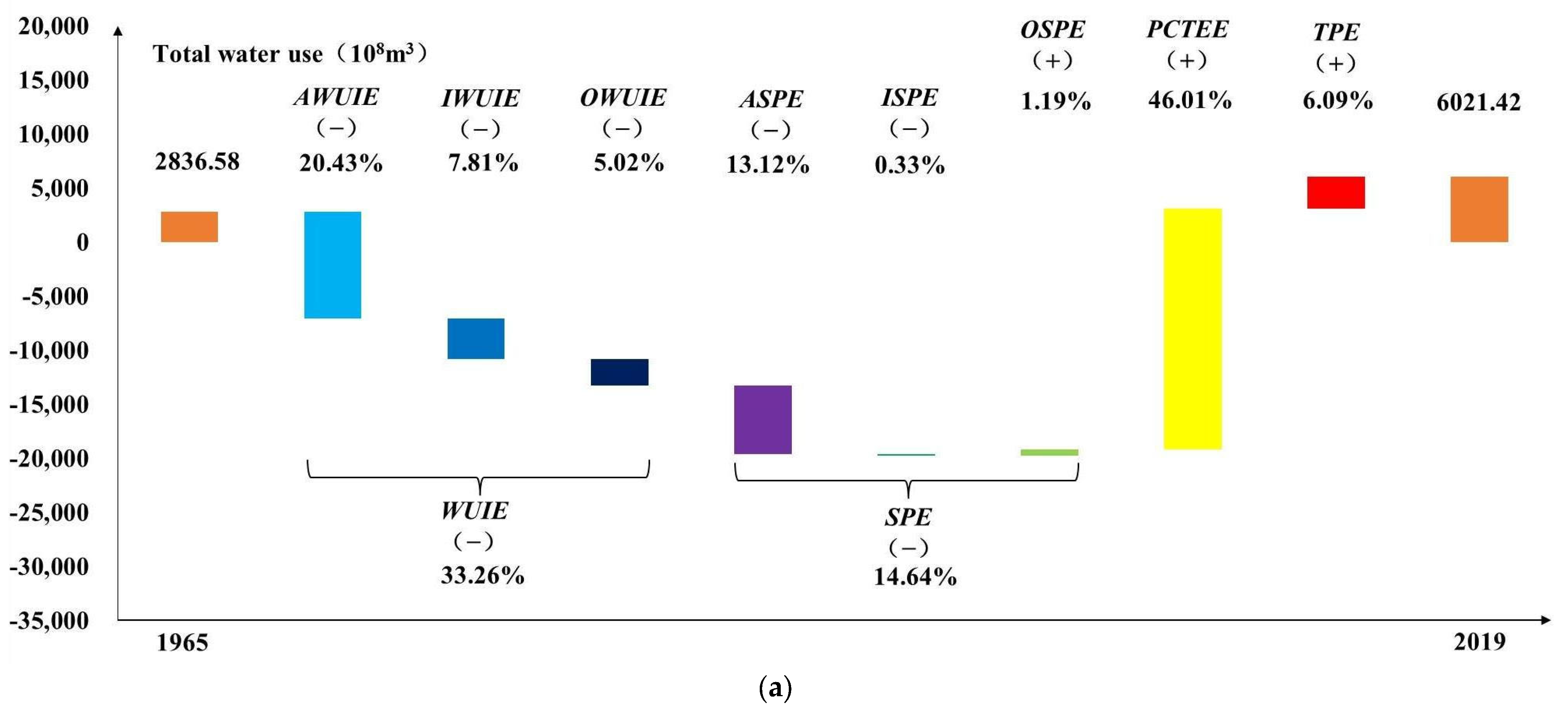
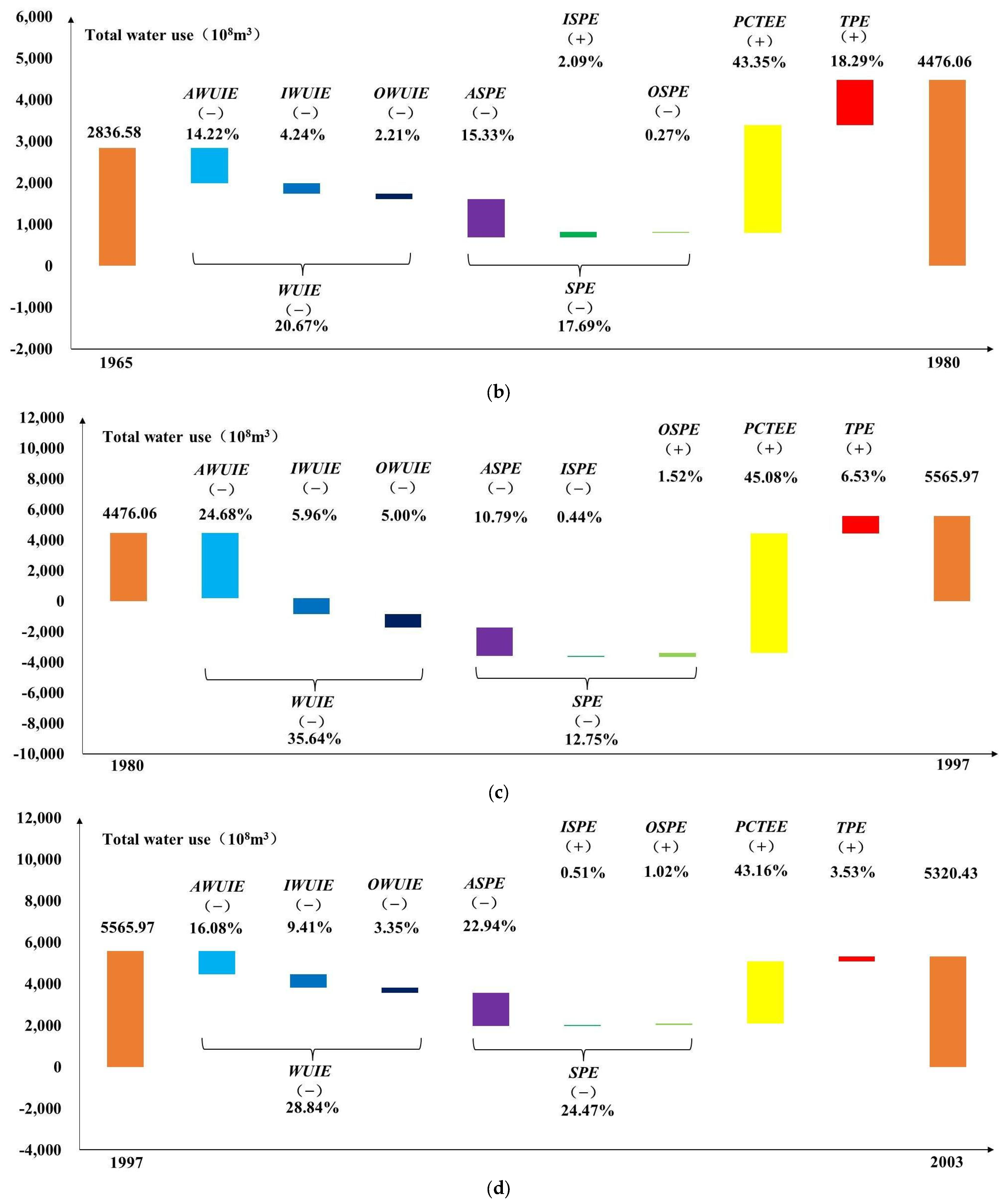
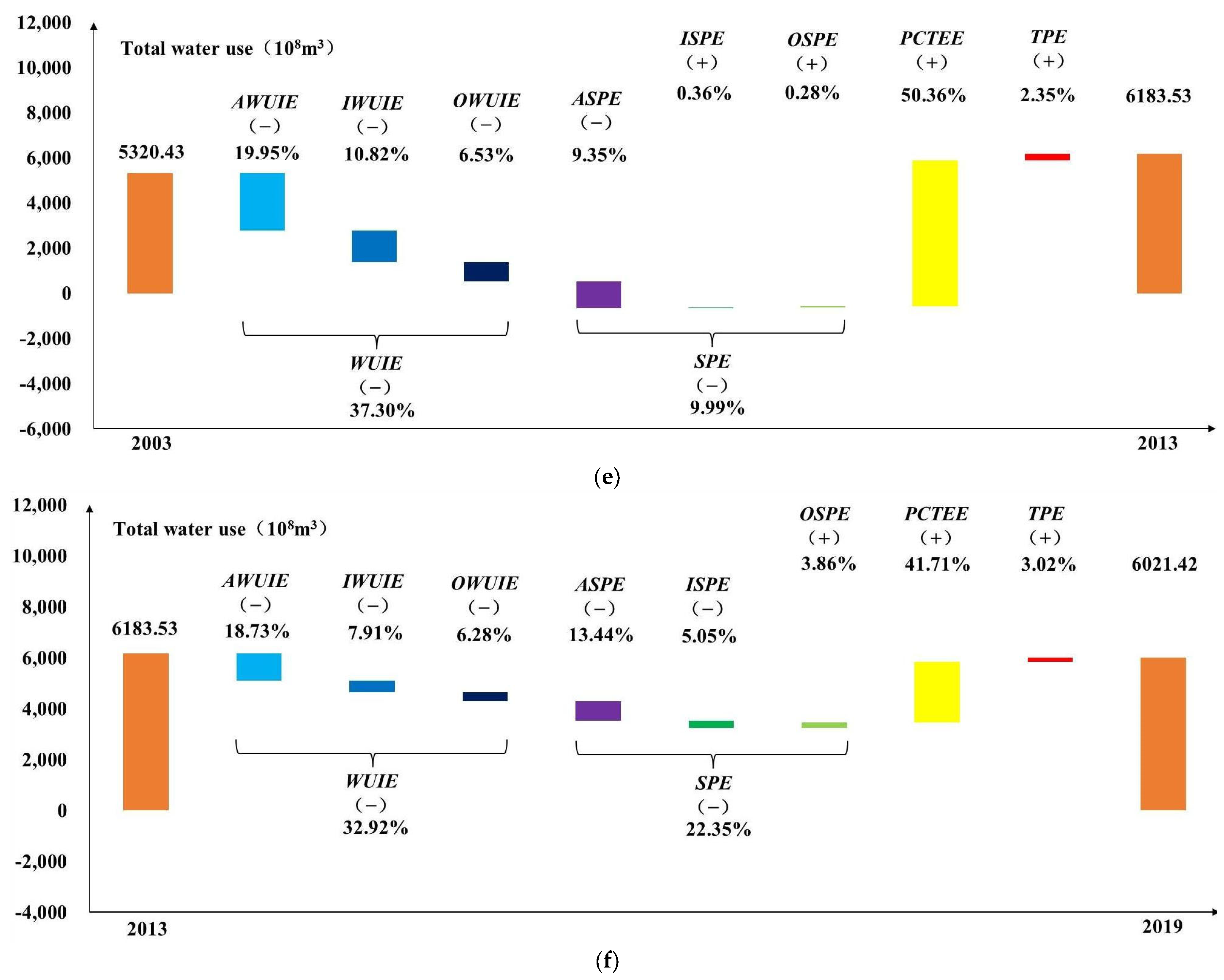
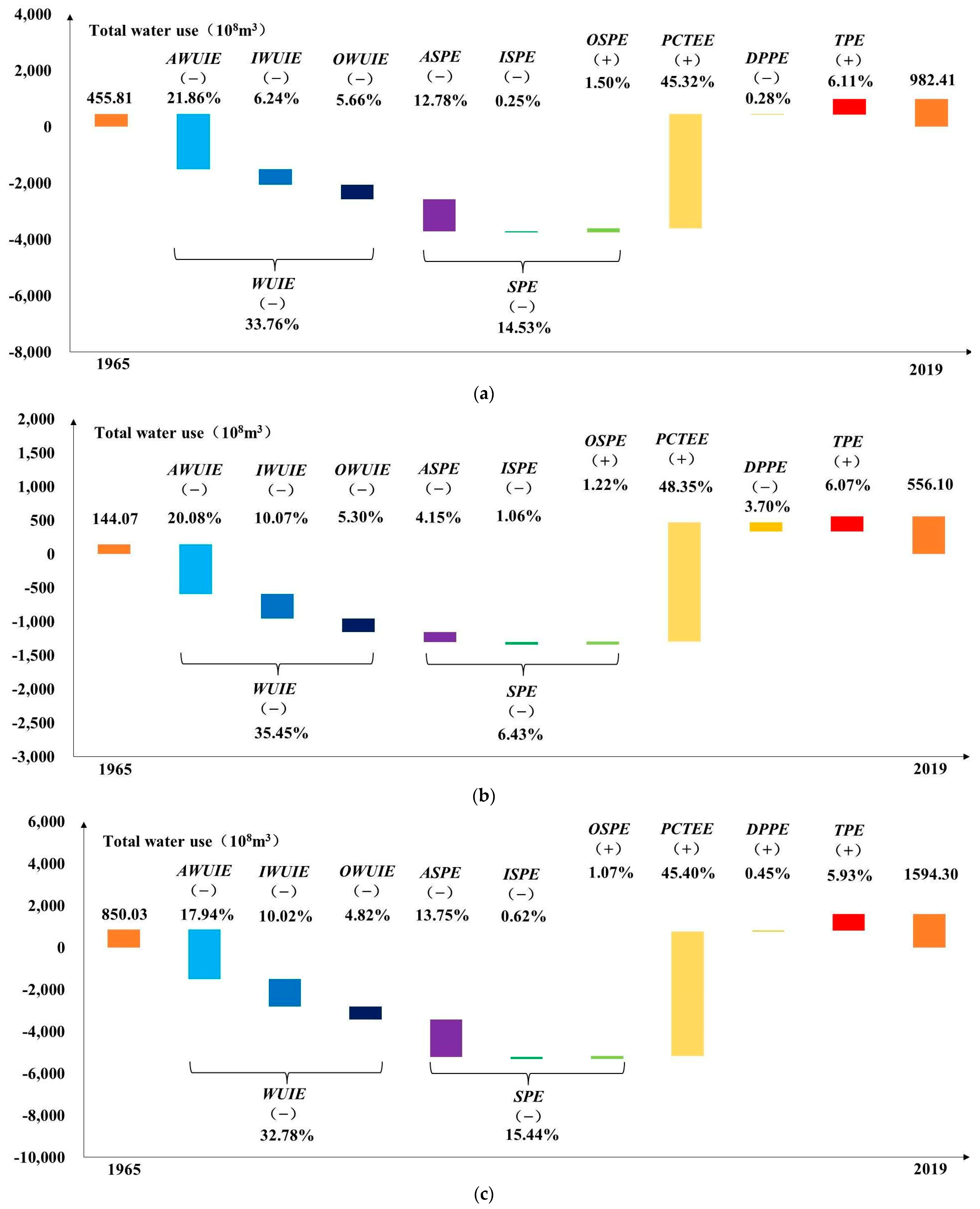
The driving effects’ proportions of the total water use evolution in China from 1965 to 2019 and its five stages were calculated (Figure 3). Comparing horizontally, the PCTEE took the maximum proportion from 1965 to 2019 and its five stages. Comparing longitudinally, the WUIE took a 33.26% proportion from 1965 to 2019, the maximum proportion in 1980–1997 (35.64%), and the minimum proportion in 1965–1980 (20.67%). The AWUIE took a 20.43% proportion from 1965 to 2019, the maximum proportion in 1980–1997 (24.68%), and the minimum proportion in 1965–1980 (14.22%). The IWUIE took a 7.81% proportion from 1965 to 2019, the maximum proportion in 2003–2013 (10.82%), and the minimum proportion in 1965–1980 (4.24%). The OWUIE took a 5.02% proportion from 1965 to 2019, the maximum proportion in 2003–2013 (6.53%), and the minimum proportion in 1965–1980 (2.21%). The SPE took a 14.64% proportion from 1965 to 2019, the maximum proportion in 1997–2003 (24.47%), and the minimum proportion in 2003–2013 (9.99%). The ASPE took a 13.12% proportion from 1965 to 2019, the maximum proportion in 1997–2003 (22.94%), and the minimum proportion in 2003–2013 (9.35%). The ISPE took a 0.33% proportion from 1965 to 2019, the maximum proportion in 2013–2019 (5.05%), and the minimum proportion in 2003–2013 (0.36%). The OSPE took a 1.19% proportion from 1965 to 2019, the maximum proportion in 2013–2019 (3.86%), and the minimum proportion in 1965–1980 (0.27%). The PCTEE took a 46.01% proportion from 1965 to 2019, the maximum proportion in 2003–2013 (50.36%), and the minimum proportion in 2013–2019 (41.71%). The TPE took a 6.09% proportion from 1965 to 2019, the maximum proportion in 1965–1980 (18.29%), and the minimum proportion in 2003–2013 (2.35%).

3.2. The Driving Effects of the Total Water Use Evolution in the Six Major Districts in China from 1965 to 2019 Considering the District Population Proportion Variable

The driving effects of the total water use evolution in the 31 provincial administrative districts in China from 1965 to 2019 considering the district population proportion variable were calculated using the LMDI-P decomposition model (

Table 3. The driving effects of the total water use evolution in the 31 provincial administrative districts in China from 1965 to 2019 considering the district population proportion variable.

District	TWUV	WUIE				SPE				PCTEE	DPPE	TPE
			AWUIE	IWUIE	OWUIE		ASPE	ISPE	OSPE
Beijing	8.10	−140.66	−62.89	−47.78	−29.99	−54.00	−52.99	−12.21	11.20	161.69	13.38	27.69
Tianjin	8.02	−94.72	−50.14	−23.80	−20.78	−23.15	−25.92	−3.44	6.21	106.71	2.26	16.92
Hebei	83.25	−690.38	−494.38	−118.41	−77.59	−224.20	−251.66	5.04	22.42	885.32	−10.85	123.36
Shanxi	35.30	−174.10	−84.88	−55.86	−33.36	−62.40	−69.89	−1.71	9.20	235.75	−3.24	39.29
Inner Mongolia	89.94	−481.81	−384.15	−43.82	−53.84	−174.15	−186.15	−0.62	12.62	676.24	−12.58	82.24
Shandong	138.59	−790.07	−491.75	−139.65	−158.67	−282.78	−324.12	1.91	39.43	1096.87	−20.00	134.57
Henan	163.43	−680.31	−402.60	−146.69	−131.02	−208.54	−244.45	3.49	32.42	936.63	−8.88	124.53
Liaoning	63.75	−465.09	−287.92	−103.05	−74.12	−71.99	−76.94	−13.72	18.67	549.54	−31.06	82.35
Jilin	85.95	−260.97	−134.17	−73.39	−53.41	−73.65	−80.69	−5.61	12.65	402.77	−30.46	48.26
Heilongjiang	262.34	−640.66	−396.13	−178.74	−65.79	65.97	77.20	−24.80	13.57	843.85	−98.07	91.25
Shanghai	25.72	−336.23	−55.03	−227.11	−54.09	−112.79	−64.46	−64.84	16.51	382.99	30.81	60.94
Jiangsu	349.08	−1553.80	−848.61	−509.42	−195.77	−636.54	−659.44	−12.06	34.96	2287.03	−19.61	272.00
Zhejiang	68.10	−621.71	−299.51	−200.46	−121.74	−280.39	−311.19	4.10	26.70	844.14	23.69	102.37
Anhui	137.70	−664.22	−422.32	−150.70	−91.20	−269.47	−302.42	8.22	24.73	956.41	−24.25	139.23
Fujian	21.06	−726.64	−468.02	−185.73	−72.89	−201.42	−227.60	14.88	11.30	812.97	32.74	103.41
Jiangxi	142.58	−469.48	−262.47	−114.66	−92.35	−228.64	−259.45	10.54	20.27	746.50	−1.39	95.59
Hubei	192.45	−710.89	−323.41	−279.75	−107.73	−226.61	−269.32	13.06	29.65	1039.65	−36.14	126.44
Hunan	115.51	−984.44	−661.35	−174.33	−148.76	−338.13	−377.00	3.73	35.14	1289.42	−44.10	192.76
Guangdong	167.59	−1366.90	−678.26	−439.40	−249.24	−523.44	−573.59	4.86	45.29	1624.95	218.45	214.53
Guangxi	181.33	−759.23	−511.00	−125.49	−122.74	−202.41	−230.39	5.25	22.73	1014.45	−0.45	128.97
Hainan	1.63	−194.21	−151.27	−15.18	−27.76	−39.54	−46.21	0.34	6.33	188.14	15.56	31.68
Chongqing	53.08	−217.28	−40.98	−116.98	−59.32	−21.11	−37.16	1.56	14.49	270.58	−9.42	30.31
Sichuan	154.28	−646.28	−323.77	−179.63	−142.88	−176.78	−223.61	8.14	38.69	904.26	−43.16	116.24
Guizhou	84.48	−195.32	−69.74	−69.25	−56.33	−45.07	−62.00	1.72	15.21	293.81	−1.84	32.90
Yunnan	79.43	−398.72	−276.81	−66.26	−55.65	−124.82	−139.24	−1.44	15.86	515.34	12.04	75.59
Tibet	26.52	−27.04	−16.76	−2.42	−7.86	−44.15	−46.40	0.73	1.52	80.81	8.23	8.67
Shaanxi	60.59	−214.52	−127.43	−38.12	−48.97	−80.02	−91.97	1.28	10.67	318.89	−4.17	40.41
Gansu	47.24	−394.26	−317.64	−49.19	−27.43	−81.78	−83.63	−5.60	7.45	462.37	−7.48	68.39
Qinghai	8.77	−75.04	−53.18	−12.42	−9.44	−30.52	−33.41	1.37	1.52	93.32	5.90	15.11
Ningxia	32.45	−171.61	−151.46	−15.41	−4.74	−119.37	−121.35	0.51	1.47	254.71	29.76	38.96
Xinjiang	296.58	−1211.59	−1178.17	−25.31	−8.11	−606.45	−614.28	−1.31	9.14	1604.28	231.70	278.64
Average	102.74	−527.68	−323.43	−126.72	−77.53	−177.37	−193.86	−1.83	18.32	705.82	7.01	94.95

). The TWUV was positive in all 31 provincial administrative districts in China, the average value was 102.74 × 10⁸ m³, the maximum value was 349.08 × 10⁸ m³ (Jiangsu), and the minimum value was 1.63 × 10⁸ m³ (Hainan). The WUIE was negative in all 31 provincial administrative districts in China, the average value was −527.68 × 10⁸ m³, the maximum value was −27.04 × 108 m3 (Tibet), and the minimum value was −1553.80 × 10⁸ m³ (Jiangsu). The AWUIE was negative value in all 31 provincial administrative districts in China, the average value was −323.43 × 10⁸ m³, the maximum value was −16.76 × 10⁸ m³ (Tibet), and the minimum value was −1178.17 × 10⁸ m³ (Xinjiang). The IWUIE was negative value in all 31 provincial administrative districts in China, the average value was −126.72 × 10⁸ m³, the maximum value was −2.42 × 10⁸ m³ (Tibet), and the minimum value was −509.42 × 10⁸ m³ (Jiangsu). The OWUIE was negative value in all 31 provincial administrative districts in China, the average value was −77.53 × 10⁸ m³, the maximum value was −4.74 × 10⁸ m³ (Ningxia), and the minimum value was −249.24 × 10⁸ m³ (Guangdong). The SPE was positive in Heilongjiang, negative in the other 30 provincial administrative districts in China, i.e., Beijing, etc., the average value was −177.37 × 10⁸ m³, the maximum value was 65.97 × 10⁸ m³ (Heilongjiang), and the minimum value was −636.54 × 10⁸ m³ (Jiangsu). The ASPE was positive in Heilongjiang and negative in the other 30 provincial administrative districts in China, i.e., Beijing, etc., the average value was −193.86×10⁸ m³, the maximum value was 77.20 × 10⁸ m³ (Heilongjiang), and the minimum value was −659.44 × 10⁸ m³ (Jiangsu). The ISPE was positive in 19 provincial administrative districts in China, i.e., Hebei, etc., negative in 12 provincial administrative districts in China, i.e., Beijing, etc., the average value was −1.83 × 10⁸ m³, the maximum value was 14.88 × 10⁸ m³ (Fujian), and the minimum value was −64.84 × 10⁸ m³ (Shanghai). The OSPE was positive in all 31 provincial administrative districts in China, the average value was 18.32 × 10⁸ m³, the maximum value was 45.29 × 10⁸ m³ (Guangdong), and the minimum value was 1.47 × 10⁸ m³ (Ningxia). The PCTEE was positive in all 31 provincial administrative districts in China, the average value was 705.82 × 10⁸ m³, the maximum value was 2287.03 × 10⁸ m³ (Jiangsu), and the minimum value was 80.81 × 10⁸ m³ (Tibet). The DPPE was positive in 12 provincial administrative districts in China, i.e., Beijing, etc., negative in the other 19 provincial administrative districts in China, i.e., Hebei, etc., the average value was 7.01 × 10⁸ m³, the maximum value was 231.70 × 10⁸ m³ (Xinjiang), and the minimum value was −98.07 × 10⁸ m³ (Heilongjiang). The TPE was positive in all 31 provincial administrative districts in China, the average value was 94.95 × 10⁸ m³, the maximum value was 278.64 × 10⁸ m³ (Xinjiang), and the minimum value was 8.67 × 10⁸ m³ (Tibet).

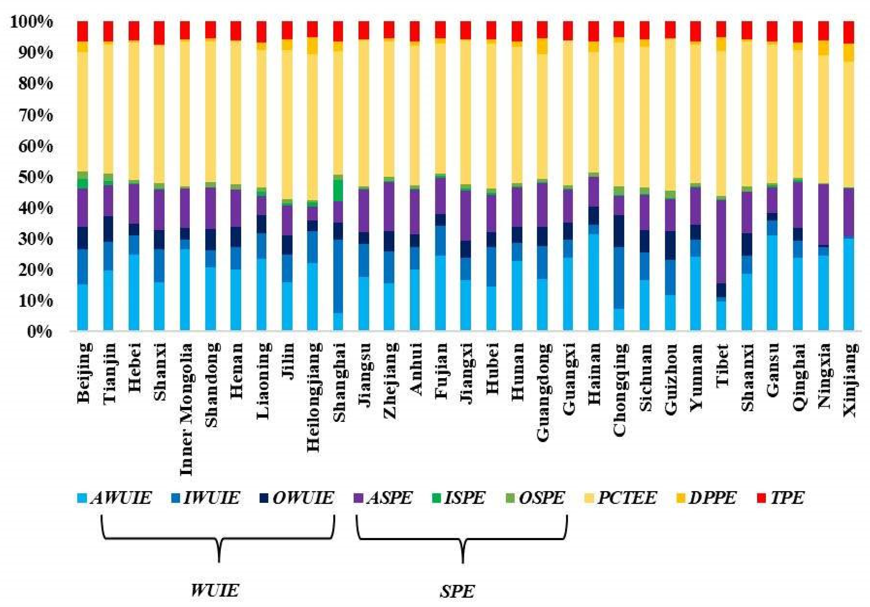
The driving effects’ proportions of the total water use evolution in the 31 provincial administrative districts in China from 1965 to 2019 considering the district population proportion variable were calculated (Figure 4). Comparing horizontally, the DPCEE took the maximum proportion in all 31 provincial administrative districts in China. Comparing longitudinally, the WUIE took the maximum proportion in Hainan (40.25%), and the minimum proportion in Tibet (15.59%). The AWUIE took the maximum proportion in Hainan (31.35%), and the minimum proportion in Shanghai (5.75%). The IWUIE took the maximum proportion in Shanghai (23.74%), and the minimum proportion in Xinjiang (0.64%). The OWUIE took the maximum proportion in Chongqing (10.21%), and the minimum proportion in Xinjiang (0.21%). The SPE took the maximum proportion in Tibet (28.06%), and the minimum proportion in Heilongjiang (6.46%). The ASPE took the maximum proportion in Tibet (26.76%), and the minimum proportion in Heilongjiang (4.31%). The ISPE took the maximum proportion in Shanghai (6.78%), and the minimum proportion in Xinjiang (0.03%). The OSPE took the maximum proportion in Beijing (2.67%), and the minimum proportion in Xinjiang (0.23%). The PCTEE took the maximum proportion in Guizhou (48.74%), and the minimum proportion in Beijing (38.51%). The DPPE took the maximum proportion in Xinjiang (5.86%), and the minimum proportion in Guangxi (0.02%). The TPE took the maximum proportion in Shanxi (7.37%), and the minimum proportion in Tibet (5.00%).

The driving effects of the total water use evolution in the six major districts in China from 1965 to 2019 considering the district population proportion variable were calculated using the LMDI-P decomposition model (

Table 4. The driving effects of the total water use evolution in the six major districts in China from 1965 to 2019 considering the district population proportion variable.

District	TWUV	WUIE				SPE				PCTEE	DPPE	TPE
			AWUIE	IWUIE	OWUIE		ASPE	ISPE	OSPE
North China	526.60	−3030.42	−1961.87	−560.30	−508.25	−1034.48	−1147.14	−22.02	134.68	4067.76	−25.06	548.80
Northeast China	412.03	−1296.95	−734.60	−368.34	−194.01	−146.09	−151.93	−38.88	44.72	1768.14	−135.11	222.04
Southeast China	744.27	−4277.75	−2340.98	−1307.46	−629.31	−1735.93	−1794.51	−80.55	139.13	5925.46	58.56	773.93
Central South China	658.53	−3990.18	−2287.61	−1032.65	−669.92	−1466.03	−1627.70	21.68	139.99	5261.54	158.47	694.73
Southwest China	397.79	−1489.08	−727.57	−436.82	−324.69	−420.12	−518.50	13.98	84.40	2090.70	−47.61	263.90
Northwest China	445.62	−2102.13	−1856.05	−144.90	−101.18	−982.40	−1010.20	−0.78	28.58	3014.47	74.06	441.62

). The TWUV was positive in all six major districts in China from 1965 to 2019, the maximum value was 744.27 × 10⁸ m³ (Southeast China), and the minimum value was 397.79 × 10⁸ m³ (Southwest China). The WUIE was negative in all six major districts in China from 1965 to 2019, the maximum value was −1296.95 × 10⁸ m³ (Northeast China), and the minimum value was −4277.75 × 10⁸ m³ (Southeast China). The AWUIE was negative in all six major districts in China from 1965 to 2019, the maximum value was −727.57 × 10⁸ m³ (Southwest China), and the minimum value was −2340.98 × 10⁸ m³ (Southeast China). The IWUIE was negative in all six major districts in China from 1965 to 2019, the maximum value was −144.90 × 10⁸ m³ (Northwest China), and the minimum value was −1307.46 × 10⁸ m³ (Southeast China). The OWUIE was negative in all six major districts in China from 1965 to 2019, the maximum value was −101.18 × 10⁸ m³ (Northwest China), and the minimum value was −669.92 × 10⁸ m³ (Central South China). The SPE was negative in all six major districts in China from 1965 to 2019, the maximum value was −146.09 × 10⁸ m³ (Northeast China), and the minimum value was −1735.93 × 10⁸ m³ (Southeast China). The ASPE was negative in all six major districts in China from 1965 to 2019, the maximum value was −151.93 × 10⁸ m³ (Northeast China), and the minimum value was −1794.51 × 10⁸ m³ (Southeast China). The ISPE was positive in two major districts in China, i.e., Central South China and Southwest China, negative in the other four major districts in China i.e., North China, Northeast China, Southeast China, and Northwest China from 1965 to 2019, the maximum value was 21.68 × 10⁸ m³ (Central South China), and the minimum value was −80.55 × 10⁸ m³ (Southeast China). The OSPE was positive in all six major districts in China from 1965 to 2019, the maximum value was 139.99 × 10⁸ m³ (Central South China), and the minimum value was 28.58 × 10⁸ m³ (Northwest China). The PCTEE was positive in all six major districts in China from 1965 to 2019, the maximum value was 5925.46 × 10⁸ m³ (Southeast China), and the minimum value was 1768.14 × 10⁸ m³ (Northeast China). The DPPE was positive in three major districts in China i.e., Southeast China, Central South China, and Northwest China, negative in the other three major districts in China i.e., North China, Northeast China, and Southwest China from 1965 to 2019, the maximum value was 158.47 × 10⁸ m³ (Central South China), and the minimum value was −135.11 × 10⁸ m³ (Northeast China). The TPE was positive in all six major districts in China from 1965 to 2019, the maximum value was 773.93 × 10⁸ m³ (Southeast China), and the minimum value was 222.04 × 10⁸ m³ (Northeast China).

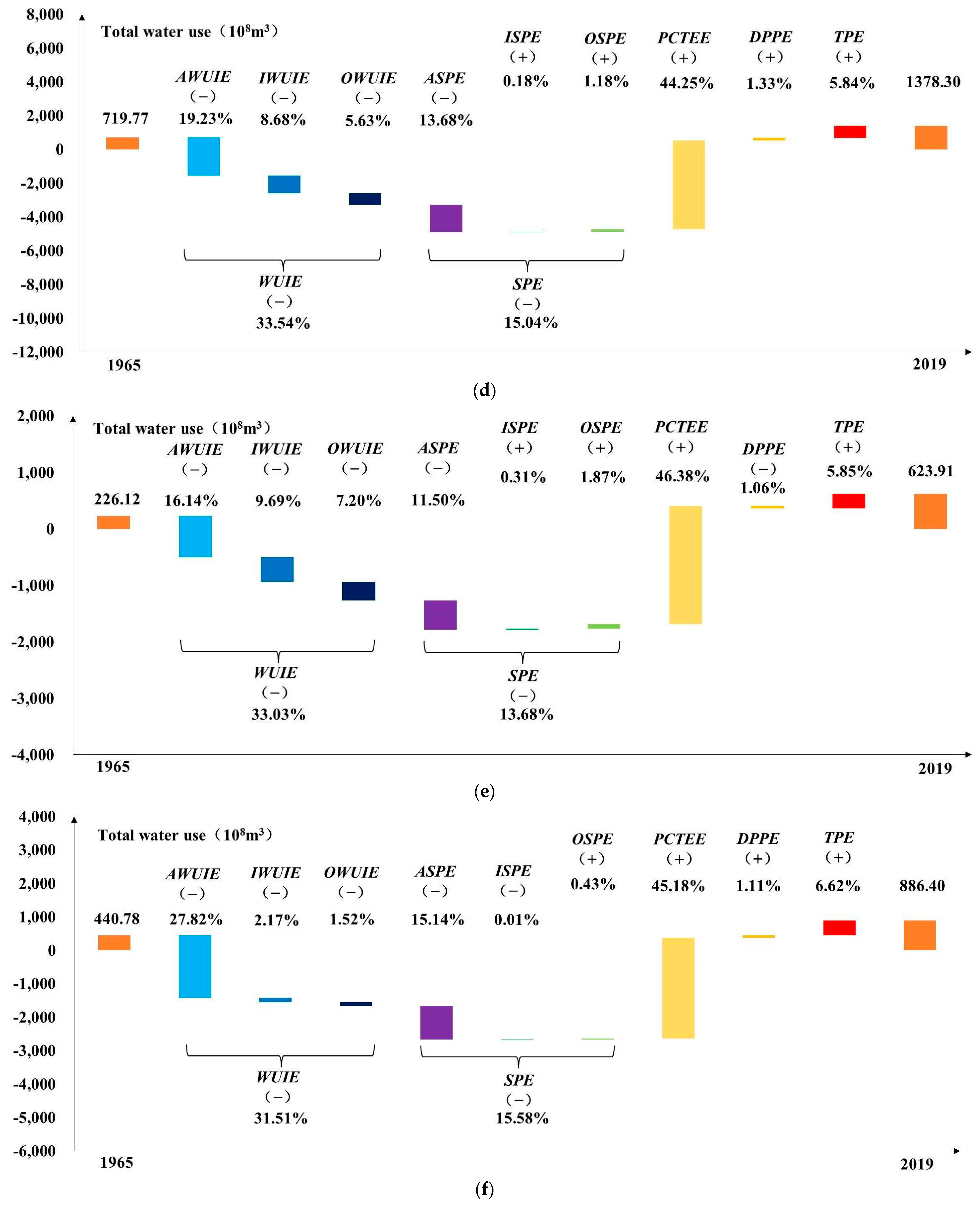
The driving effects’ proportions of the total water use evolution proportions in the six major districts in China from 1965 to 2019 considering the district population proportion variable were calculated (Figure 5). Comparing horizontally, the PCTEE took the maximum proportion in all six major districts in China from 1965 to 2019. Comparing longitudinally, the WUIE took the maximum proportion in Northeast China (35.45%), and the minimum proportion in Northwest China (31.51%). The AWUIE took the maximum proportion in Northwest China (27.82%), and the minimum proportion in Southwest China (16.14%). The IWUIE took the maximum proportion in Northeast China (10.07%), and the minimum proportion in Northwest China (2.17%). The OWUIE took the maximum proportion in Southwest China (7.20%), and the minimum proportion in Northwest China (1.52%). The SPE took the maximum proportion in Northwest China (15.58%), and the minimum proportion in Northeast China (6.43%). The ASPE took the maximum proportion in Northwest China (15.14%), and the minimum proportion in Northeast China (4.15%). The ISPE took the maximum proportion in Northeast China (1.06%), and the minimum proportion in Northwest China (0.01%). The OSPE took the maximum proportion in Southwest China (1.87%), and the minimum proportion in Northwest China (0.43%). The PCTEE took the maximum proportion in Northeast China (48.35%), and the minimum proportion in Central South China (44.25%). The DPPE took the maximum proportion in Northeast China (3.70%), and the minimum proportion in North China (0.28%). The TPE took the maximum proportion in Northwest China (6.62%), and the minimum proportion in Central South China (5.84%).

3.3. The Driving Effects of the Total Water Use Evolution in the Six Major Districts in China from 1965 to 2019 Considering the District Economic Proportion Variable

The driving effects of the total water use evolution in the 31 provincial administrative districts in China from 1965 to 2019 considering the district economic proportion variable were calculated using the LMDI-E decomposition model (

Table 5. The driving effects of the total water use evolution in the 31 provincial administrative districts in China from 1965 to 2019 considering the district economic proportion variable.

District	TWUV	WUIE				SPE				DEPE	PCTEE	TPE
			AWUIE	IWUIE	OWUIE		ASPE	ISPE	OSPE
Beijing	8.10	−140.66	−62.89	−47.78	−29.99	−54.00	−52.99	−12.21	11.20	1.78	173.29	27.69
Tianjin	8.02	−94.72	−50.14	−23.80	−20.78	−23.15	−25.92	−3.44	6.21	2.08	106.89	16.92
Hebei	83.25	−690.38	−494.38	−118.41	−77.59	−224.20	−251.66	5.04	22.42	9.67	864.80	123.36
Shanxi	35.30	−174.10	−84.88	−55.86	−33.36	−62.40	−69.89	−1.71	9.20	−34.15	266.66	39.29
Inner Mongolia	89.94	−481.81	−384.15	−43.82	−53.84	−174.15	−186.15	−0.62	12.62	27.72	635.94	82.24
Shandong	138.59	−790.07	−491.75	−139.65	−158.67	−282.78	−324.12	1.91	39.43	91.81	985.06	134.57
Henan	163.43	−680.31	−402.60	−146.69	−131.02	−208.54	−244.45	3.49	32.42	5.28	922.47	124.53
Liaoning	63.75	−465.09	−287.92	−103.05	−74.12	−71.99	−76.94	−13.72	18.67	−66.78	585.26	82.35
Jilin	85.95	−260.97	−134.17	−73.39	−53.41	−73.65	−80.69	−5.61	12.65	−36.11	408.42	48.26
Heilongjiang	262.34	−640.66	−396.13	−178.74	−65.79	65.97	77.20	−24.80	13.57	−172.31	918.09	91.25
Shanghai	25.72	−336.23	−55.03	−227.11	−54.09	−112.79	−64.46	−64.84	16.51	−22.71	436.51	60.94
Jiangsu	349.08	−1553.80	−848.61	−509.42	−195.77	−636.54	−659.44	−12.06	34.96	245.08	2022.34	272.00
Zhejiang	68.10	−621.71	−299.51	−200.46	−121.74	−280.39	−311.19	4.10	26.70	78.80	789.03	102.37
Anhui	137.70	−664.22	−422.32	−150.70	−91.20	−269.47	−302.42	8.22	24.73	−49.95	982.11	139.23
Fujian	21.06	−726.64	−468.02	−185.73	−72.89	−201.42	−227.60	14.88	11.30	95.98	749.73	103.41
Jiangxi	142.58	−469.48	−262.47	−114.66	−92.35	−228.64	−259.45	10.54	20.27	−37.53	782.64	95.59
Hubei	192.45	−710.89	−323.41	−279.75	−107.73	−226.61	−269.32	13.06	29.65	−26.65	1030.16	126.44
Hunan	115.51	−984.44	−661.35	−174.33	−148.76	−338.13	−377.00	3.73	35.14	−98.12	1343.44	192.76
Guangdong	167.59	−1366.90	−678.26	−439.40	−249.24	−523.44	−573.59	4.86	45.29	180.23	1663.17	214.53
Guangxi	181.33	−759.23	−511.00	−125.49	−122.74	−202.41	−230.39	5.25	22.73	−39.28	1053.28	128.97
Hainan	1.63	−194.21	−151.27	−15.18	−27.76	−39.54	−46.21	0.34	6.33	2.76	200.94	31.68
Chongqing	53.08	−217.28	−40.98	−116.98	−59.32	−21.11	−37.16	1.56	14.49	7.27	253.89	30.31
Sichuan	154.28	−646.28	−323.77	−179.63	−142.88	−176.78	−223.61	8.14	38.69	−23.82	884.92	116.24
Guizhou	84.48	−195.32	−69.74	−69.25	−56.33	−45.07	−62.00	1.72	15.21	−12.70	304.67	32.90
Yunnan	79.43	−398.72	−276.81	−66.26	−55.65	−124.82	−139.24	−1.44	15.86	−36.60	563.98	75.59
Tibet	26.52	−27.04	−16.76	−2.42	−7.86	−44.15	−46.40	0.73	1.52	2.33	86.71	8.67
Shaanxi	60.59	−214.52	−127.43	−38.12	−48.97	−80.02	−91.97	1.28	10.67	2.22	312.50	40.41
Gansu	47.24	−394.26	−317.64	−49.19	−27.43	−81.78	−83.63	−5.60	7.45	−36.57	491.46	68.39
Qinghai	8.77	−75.04	−53.18	−12.42	−9.44	−30.52	−33.41	1.37	1.52	−11.95	111.17	15.11
Ningxia	32.45	−171.61	−151.46	−15.41	−4.74	−119.37	−121.35	0.51	1.47	−18.11	302.58	38.96
Xinjiang	296.58	−1211.59	−1178.17	−25.31	−8.11	−606.45	−614.28	−1.31	9.14	−177.19	2013.17	278.64
Average	102.74	−527.68	−323.43	−126.72	−77.53	−177.37	−193.86	−1.83	18.32	−4.76	717.59	94.95

). The DEPE was positive in 14 provincial administrative districts in China, i.e., Beijing, etc., and negative in the other 17 provincial administrative districts in China, i.e., Shanxi, etc., the average value was −4.76 × 10⁸ m³, the maximum value was 245.08 × 10⁸ m³ (Jiangsu), and the minimum value was −177.19 × 10⁸ m³ (Xinjiang). The PCTEE was positive in all 31 provincial administrative districts in China, the average value was 717.59 × 10⁸ m³, the maximum value was 2022.34 × 10⁸ m³ (Jiangsu), and the minimum value was 86.71 × 10⁸ m³ (Tibet). The other results are consistent with Table 3.

The driving effects’ proportions of the total water use evolution in the 31 provincial administrative districts in China from 1965 to 2019 considering the district economic proportion variable were calculated (Figure 6). Comparing horizontally, the PCTEE took the maximum proportion in all 31 provincial administrative districts in China. Comparing longitudinally, the WUIE took the maximum proportion in Hainan (40.25%), and the minimum proportion in Tibet (15.59%). The AWUIE took the maximum proportion in Hainan (31.35%), and the minimum proportion in Shanghai (5.49%). The IWUIE took the maximum proportion in Shanghai (22.66%), and the minimum proportion in Xinjiang (0.59%). The OWUIE took the maximum proportion in Chongqing (10.56%), and the minimum proportion in Xinjiang (0.19%). The SPE took the maximum proportion in Tibet (28.06%), and the minimum proportion in Heilongjiang (5.96%). The ASPE took the maximum proportion in Tibet (26.76%), and the minimum proportion in Heilongjiang (3.98%). The ISPE took the maximum proportion in Shanghai (6.47%), and the minimum proportion in Xinjiang (0.03%). The OSPE took the maximum proportion in Beijing (2.67%), and the minimum proportion in Xinjiang (0.21%). The DEPE took the maximum proportion in Heilongjiang (8.89%), and the minimum proportion in Henan (0.26%). The PCTEE took the maximum proportion in Tibet (50.01%), and the minimum proportion in Fujian (38.86%). The TPE took the maximum proportion in Tianjin (6.60%), and the minimum proportion in Heilongjiang (4.71%).

The driving effects of the total water use evolution in the six major districts in China from 1965 to 2019 considering the district economic proportion variable were calculated using the LMDI-E decomposition model (

Table 6. The driving effects of the total water use evolution in the six major districts in China from 1965 to 2019 considering the district economic proportion variable.

District	TWUV	WUIE				SPE				DEPE	PCTEE	TPE
			AWUIE	IWUIE	OWUIE		ASPE	ISPE	OSPE
North China	526.60	−3030.42	−1961.87	−560.30	−508.25	85.62	3957.08	−22.02	134.68	85.62	3957.08	548.80
Northeast China	412.03	−1296.95	−734.60	−368.34	−194.01	−280.33	1913.36	−38.88	44.72	−280.33	1913.36	222.04
Southeast China	744.27	−4277.75	−2340.98	−1307.46	−629.31	218.55	5765.47	−80.55	139.13	218.55	5765.47	773.93
Central South China	658.53	−3990.18	−2287.61	−1032.65	−669.92	124.09	5295.92	21.68	139.99	124.09	5295.92	694.73
Southwest China	397.79	−1489.08	−727.57	−436.82	−324.69	−53.88	2096.97	13.98	84.40	−53.88	2096.97	263.90
Northwest China	445.62	−2102.13	−1856.05	−144.90	−101.18	−143.53	3232.06	−0.78	28.58	−143.53	3232.06	441.62

). The DEPE was positive in three major districts in China i.e., North China, Southeast China, and Central South China, negative in the other three major districts in China i.e., Northeast China, Southwest China, and Northwest China from 1965 to 2019, the maximum value was 218.55 × 10⁸ m³ (Southeast China), and the minimum value was −280.33 × 10⁸ m³ (Northeast China). The PCTEE was positive in all six major districts in China from 1965 to 2019, the maximum value was 5765.47×10⁸ m³ (Southeast China), and the minimum value was 1913.36 × 10⁸ m³ (Northeast China). The other results are consistent with Table 4.

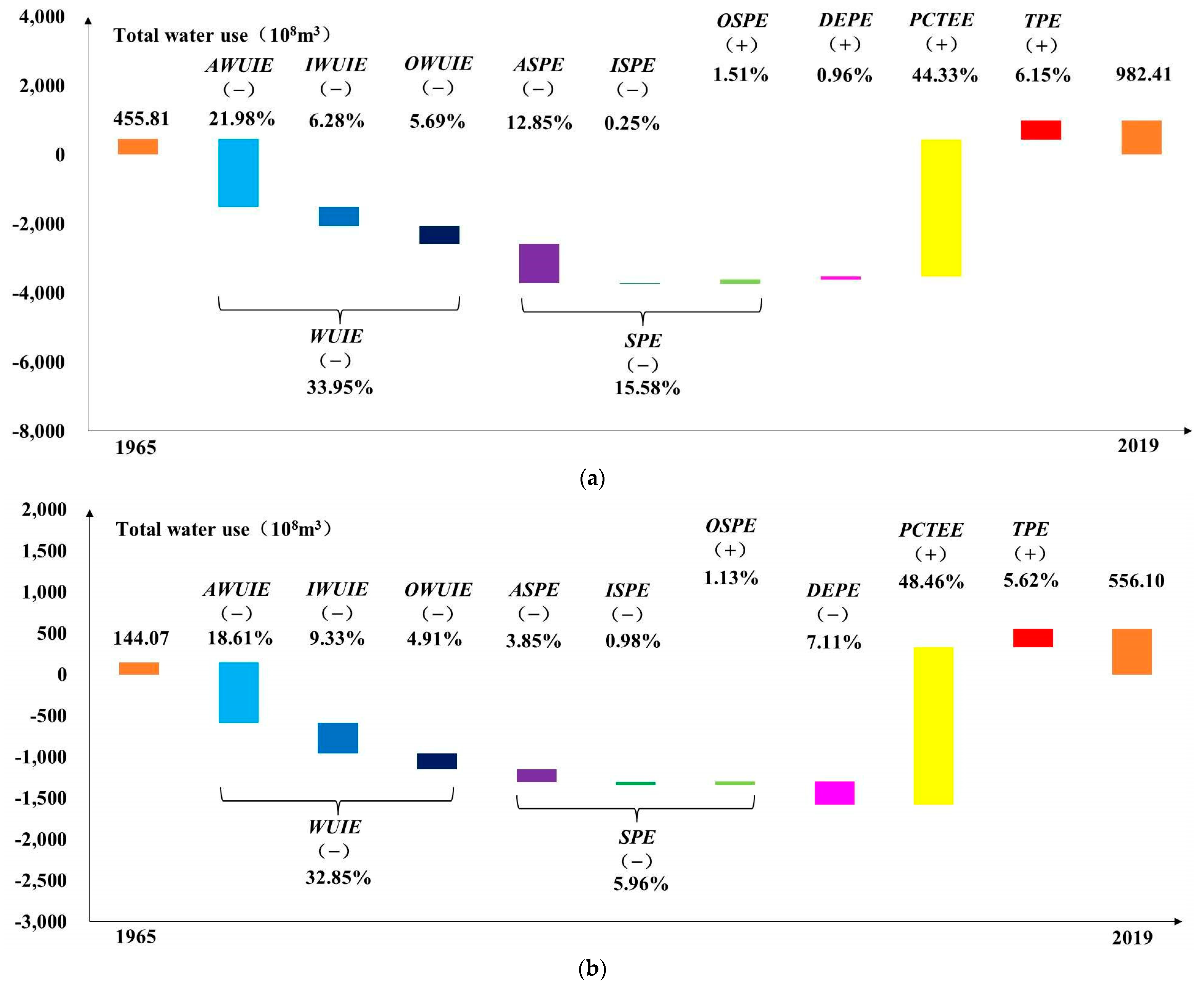
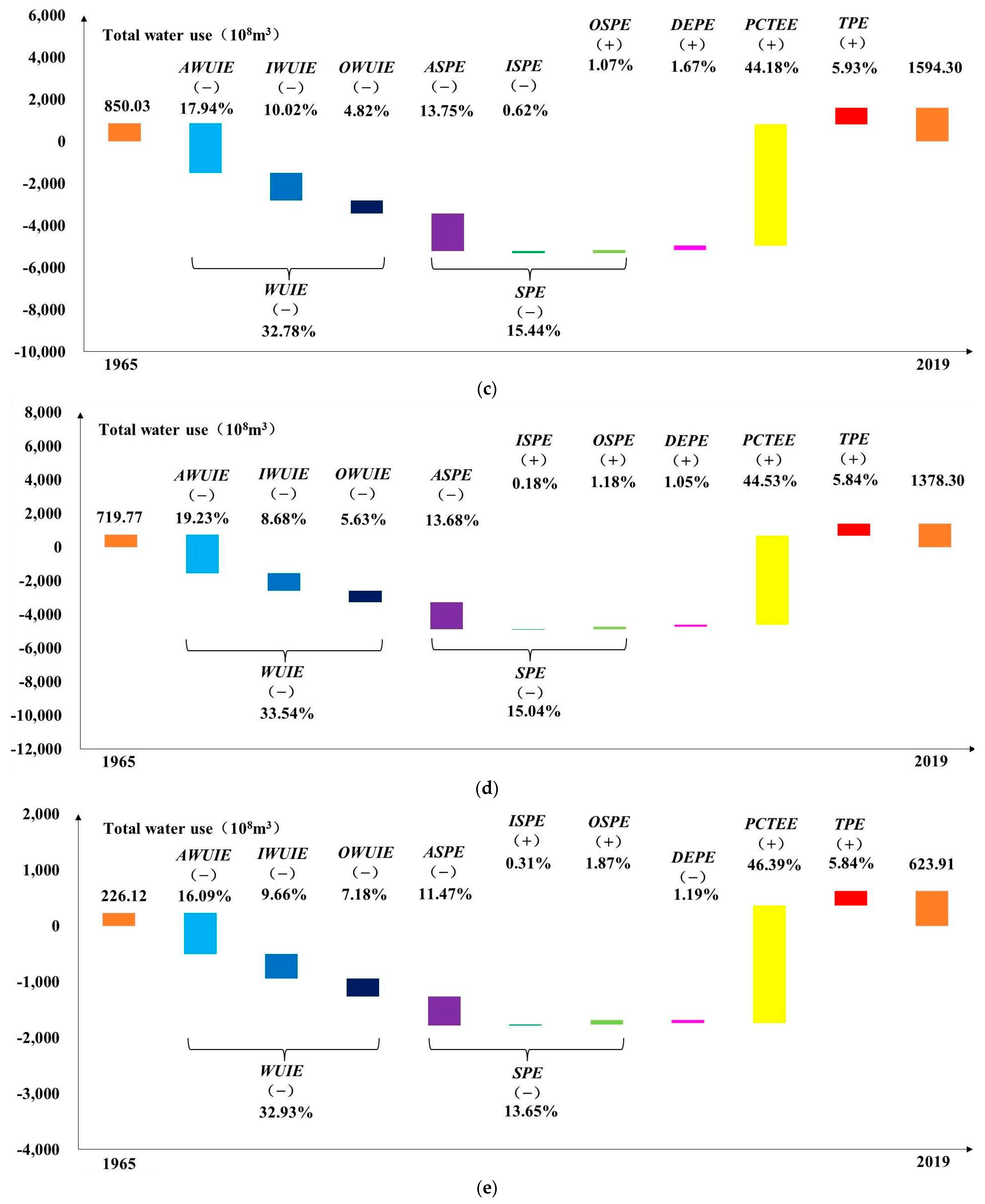
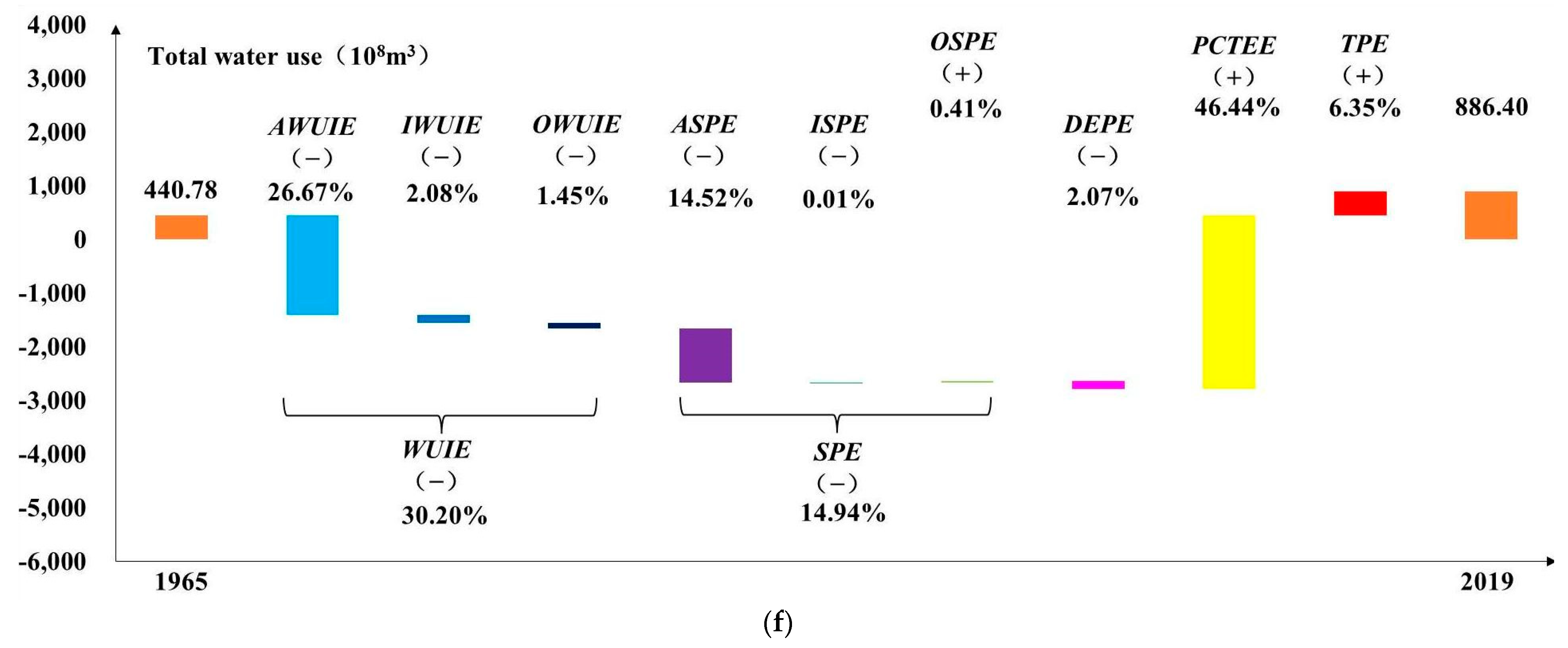
The driving effects’ proportions of the total water use evolution in the six major districts in China from 1965 to 2019 considering the district economic proportion variable were calculated (Figure 7). Comparing horizontally, the PCTEE took the maximum proportion in all 6 major districts in China from 1965 to 2019. Comparing longitudinally, the WUIE took the maximum proportion in North China (33.95%), and the minimum proportion in Northwest China (30.20%). The AWUIE took the maximum proportion in Northwest China (26.67%), and the minimum proportion in Southwest China (16.09%). The IWUIE took the maximum proportion in Southeast China (10.02%), and the minimum proportion in Northwest China (2.08%). The OWUIE took the maximum proportion in Southwest China (7.18%), and the minimum proportion in Northwest China (1.45%). The SPE took the maximum proportion in Southeast China (15.44%), and the minimum proportion in Northeast China (5.96%). The ASPE took the maximum proportion in Northwest China (14.52%), and the minimum proportion in Northeast China (3.85%). The ISPE took the maximum proportion in Northeast China (0.98%), and the minimum proportion in Northwest China (0.01%). The OSPE took the maximum proportion in Southwest China (1.87%), and the minimum proportion in Northwest China (0.41%). The DEPE took the maximum proportion in Northeast China (7.11%), and the minimum proportion in North China (0.96%). The PCTEE took the maximum proportion in Northeast China (48.46%), and the minimum proportion in Southeast China (44.18%). The TPE took the maximum proportion in Northwest China (6.35%), and the minimum proportion in Northeast China (5.62%).

4. Discussion

4.1. Analysis of the Driving Effects of the Total Water Use Evolution in China from 1965 to 2019 and Its Five Stages

Compared with the existing literature [29,30,31,32], in this research, we studied the driving effects of the total water use evolution in China from the perspective of multi-year long time-series in the whole country for the first time. This could comprehensively explain the influence mechanism of the total water use evolution in China. Through the results calculated using the LMDI decomposition model, both the WUIE and SPE played an inhibitive role with respect to the total water use increasing in China from 1965 to 2019 and its five stages, and both the PCTEE and TPE played a prohibitive role with respect to the total water use increasing in China from 1965 to 2019 and its five stages. We analyzed the influence mechanisms of the driving effects of the total water use evolution in China from 1965 to 2019 and its five stages (

Table 7. The influence mechanisms of the driving effects of the total water use evolution in China from 1965 to 2019 and its five stages.

Driving Effect	Data Example	Influence Mechanism
WUIE	The agricultural, industrial, and other sector water use intensity separately decreased from 3.67 × 10−2 m3/million CNY, 0.55 × 10−2 m3/million CNY, and 0.63 × 10−2 m3/million CNY in 1965 to 0.25 × 10−2 m3/million CNY, 0.02 × 10−2 m3/million CNY, and 0.01 × 10−2 m3/million CNY in 2019.	The innovation and application of water-saving technology is conducive to improving the water use efficiency in different sectors; the emerging irrigation technology is conducive to improving the effective coefficient of irrigative water utilization; the development of industrial clean technology is conducive to improving the reuse rate of industrial water; and the in-depth awareness of citizens with respect to water-saving is conducive to improving the domestic water use efficiency, thus reducing the total water use.
SPE	The proportion of the agricultural, industrial, and other sector added value to the gross domestic product changed from 41:38:21 in 1965 to 7:39:54 in 2019.	With the economic development, the sector structure is optimized and upgraded, the center of gravity of the sector structure shifts from agriculture to industry and other sector, and both the industrial and other sector water use efficiency are significantly higher than the agricultural water use efficiency, thus reducing the total water use.
PCTEE	The per capita gross domestic product increased from 213.13 CNY per person in 1965 to 14832.75 CNY per person in 2019.	As the economic strength increases year by year, water resources offer irreplaceable basic support for socio-economic development and represent an indispensable production factor, thus increasing the total water use.
TPE	The total population increased from 725 million in 1965 to 1.4 billion in 2019.	The increasing population will inevitably increase household consumption and lead to a larger scale of economic production, thus increasing the total water use.

).

4.2. Analysis of the DPPE and DEPE of the Total Water Use Evolution in the Six Major Districts in China from 1965 to 2019

Compared with the existing literature [29,30,31,32], in this research, we also considered the driving effects of the total water use evolution when the population or economic proportion changed in the six major districts in China for the first time. This could comprehensively reflect the actual water demand in these districts. Through the results calculated using the LMDI-P decomposition model, the DPPE played a prohibitive role in Southeast China, Central South China, and Northwest China with respect to the total water use increasing, and an inhibitive role in North China, Northeast China, and Southwest China with respect to the total water use increasing. Similarly, through the results calculated using the LMDI-E decomposition model, the DEPE played a prohibitive role in North China, Southeast China, and Central South China with respect to the total water use increasing, and an inhibitive role in Northeast China, Southwest China, and Northwest China with respect to the total water use increasing. We analyzed the influence mechanisms of the DPPE and the DEPE with respect to the total water use evolution in the six major districts in China from 1965 to 2019 (

Table 8. The influence mechanisms of the DPPE and DEPE with respect to the total water use evolution in China from 1965 to 2019.

Driving Effect	Data Example	Influence Mechanism
DPPE	The total population proportion of Southeast China, Central South China, and Northwest China separately increased from 22.06%, 19.50%, and 6.58% in 1965 to 22.78%, 22.04%, and 7.33% in 2019, while the total population proportion of North China, Northeast China, and Southwest China separately decreased from 27.18%, 9.11%, and 15.59% in 1965 to 26.24%, 7.09%, and 14.53% in 2019.	China has successively introduced some regional economic development strategies such as “Reform and Opening up” and “Western Development”; consequently, there appears to be a certain population flow phenomenon, and its path generally moves from the population outflow district (North China, Northeast China, and Southwest China) to the population inflow district (Southeast China, Central South China, and Northwest China), resulting in the total population proportion of the six major districts in China changing. The total water use in the population inflow district has increased with the total population proportion increasing, and in the population outflow district it has decreased with the total population proportion decreasing.
DEPE	The gross regional product proportion of North China, Southeast China, and Central South China separately increased from 23.75%, 26.29%, and 18.37% in 1965 to 26.88%, 31.25%, and 19.69% in 2019, while the gross regional product proportion of Northeast China, Southwest China, and Northwest China separately decreased from 13.72%, 11.65%, and 6.22% in 1965 to 7.65%, 9.53%, and 5.00% in 2019.	Although China has introduced some regional economic development strategies, the economic development of the six major districts in China is still unbalanced, the economically developed district (North China, Southeast China, and Central South China) has a faster economic growth rate, and the economically underdeveloped district (Northeast China, Southwest China, and Northwest China) has a slower economic growth rate, resulting in the gross regional product proportion of the six major districts in China changing. The total water use in the economically developed district has increased with the economic proportion increasing, and in the economically underdeveloped district, it has decreased with the economic proportion decreasing.

).

5. Conclusions and Prospects

5.1. Conclusions

In this research, we studied the driving effects of the total water use evolution in China from the perspective of multi-year long time-series in the whole country for the first time. This could comprehensively explain the influence mechanism of the total water use evolution in China and provide a complete research example for scholars studying related fields in other countries. Through the LMDI decomposition method, we constructed an LMDI decomposition model for the regional total water use evolution, and decomposed the total water use evolution in China and its five stages from 1965 to 2019 into the WUIE, SPE, PCTEE, and TPE. We calculated the value and proportion of the driving effects of the total water use evolution in China, and the results indicate that according to the overall situation from 1965 to 2019, the prohibitive role played by the PCTEE (total 22,263.79 × 10⁸ m³) and the TPE (total 2945.38 × 10⁸ m³) with respect to the total water use increasing in China offset the inhibitive role played by the WUIE (total −16,094.31 × 10⁸ m³) and the SPE (total −5930.02 × 10⁸ m³) with respect to the total water use increasing in China.

In this research, we also considered the driving effects of the total water use evolution when the population or economic proportion changed in the six major districts in China for the first time. This could comprehensively reflect the actual water demand in these districts. Based on the LMDI decomposition method, we separately added the district population (economic) proportion variable to construct an LMDI-P (LMDI-E) decomposition model for the regional total water use evolution. Compared with the LMDI decomposition model, the DPPE and DEPE were separately added. We calculated the value and proportion of the two driving effects of the total water use evolution in the six major districts in China, and the results indicate that according to the overall situation from 1965 to 2019, both the DPPE and DEPE had heterogeneity in the total water use evolution in the six major districts in China. The DPPE played a prohibitive role in the three population inflow districts (Southeast China, Central South China, and Northwest China) with respect to the total water use increasing (total 291.09 × 10⁸ m³), and an inhibitive role in the other three population outflow districts (North China, Central South China, and Southwest China) with respect to the total water use increasing (total −207.78 × 10⁸ m³). The DEPE played a prohibitive role in the three economically developed districts (North China, Southeast China, and Central South China) with respect to the total water use increasing (total 428.26 × 10⁸ m³), and an inhibitive role in the other three economically underdeveloped districts (Northeast China, Southwest China, and Northwest China) with respect to the total water use increasing (total −477.74 × 10⁸ m³).

5.2. Prospects

In this research, through the LMDI decomposition method, the total water use evolution in China from 1965 to 2019 was decomposed into multiple the driving effects, comprehensively summarizing the driving effects of the total water use evolution. However, the influence mechanism of the total water use evolution is still relatively complex, with many driving effects, which are not limited to the driving effects proposed in this research. In addition, based on the consideration of data availability, using the LMDI decomposition method to decompose the total water use into multiple driving effects has a certain subjectivity. In future research, it will be necessary to examine the influence mechanism of the total water use evolution more deeply and identify the driving effects more comprehensively. For example, how do climate change and China’s recent water-saving policies influence the total water use evolution in China? We should also quantify the value and proportion of the driving effects on the total water use evolution with relatively objective models, such as the generalized Divisia index method (GDIM) model [33] and the random forest model [34], to better provide decision-making references for the planning and management of water resource in various regions of China.

References

1. Shahsavari-Pour, N.; Bahador, S.; Heydari, A.; Fekih, A. Water Shortage Simulation Using a System Dynamics Approach: A Case Study of the Rafsanjan City. Sustainability 2023, 15, 6225. [Google Scholar] [CrossRef]
2. Tang, X.; He, Y.; Qi, P.; Chang, Z.; Jiang, M.; Dai, Z. A New Multi-Objective Optimization Model of Water Resources Considering Fairness and Water Shortage Risk. Water 2021, 13, 2648. [Google Scholar] [CrossRef]
3. Ren, K.; Huang, S.; Huang, Q.; Wang, H.; Leng, G.; Cheng, L.; Fang, W.; Li, P. A Nature-Based Reservoir Optimization Model for Resolving the Conflict in Human Water Demand and Riverine Ecosystem Protection. J. Clean. Prod. 2019, 231, 406–418. [Google Scholar] [CrossRef]
4. Aba, M.M.; Parente, V.; dos Santos, E.M. Estimation of Water Demand of the Three Major Brazilian Shale-Gas Basins: Implications for Water Availability. Energy Policy 2022, 168, 113170. [Google Scholar] [CrossRef]
5. He, C.; Liu, Z.; Wu, J.; Pan, X.; Fang, Z.; Li, J.; Bryan, B.A. Future Global Urban Water Scarcity and Potential Solutions. Nat. Commun. 2021, 12, 4667. [Google Scholar] [CrossRef]
6. Sun, S.; Zhou, X.; Liu, H.; Jiang, Y.; Zhou, H.; Zhang, C.; Fu, G. Unraveling the Effect of Inter-Basin Water Transfer on Reducing Water Scarcity and Its Inequality in China. Water Res. 2021, 194, 116931. [Google Scholar] [CrossRef]
7. Gleick, P.H. Water Use. Annu. Rev. Environ. Resour. 2003, 28, 275–314. [Google Scholar] [CrossRef]
8. Gleick, P.H.; Palaniappan, M. Peak Water Limits to Freshwater Withdrawal and Use. Proc. Natl. Acad. Sci. USA 2010, 107, 11155–11162. [Google Scholar] [CrossRef] [PubMed]
9. Han, J.; Wang, C.; Deng, S.; Lichtfouse, E. China’s Sponge Cities Alleviate Urban Flooding and Water Shortage: A Review. Environ. Chem. Lett. 2023, 21, 1297–1314. [Google Scholar] [CrossRef]
10. Sheng, J.; Webber, M. Do Water-Saving Policies Improve Water-Use Technical Efficiency? Evidence from the Water-Receiving Cities of China’s South-North Water Transfer Project. J. Environ. Policy Plan. 2023, 25, 493–509. [Google Scholar] [CrossRef]
11. Zhang, S.; Fu, H.; Wang, Y. The Impact of the Water Commonweal Propaganda on Citizens’ Water-Saving Behavior: The Intermediary Role of Propaganda Channels and Forms—Evidence from China. Water Policy 2021, 23, 1468–1488. [Google Scholar] [CrossRef]
12. Zhao, J. The Cubic Water Kuznets Curve: Patterns of Urban Water use and Water Policy Effects. Water Policy 2017, 19, 28–45. [Google Scholar] [CrossRef]
13. Zhang, C.; Zhong, L.; Wang, J. Decoupling between Water Use and Thermoelectric Power Generation Growth in China. Nat. Energy 2018, 3, 792–799. [Google Scholar] [CrossRef]
14. Zhao, L.; Sun, C.; Liu, F. Interprovincial Two-Stage Water Resource Utilization Efficiency under Environmental Constraint and Spatial Spillover Effects in China. J. Clean. Prod. 2017, 164, 715–725. [Google Scholar] [CrossRef]
15. Ma, H.; Shi, C.; Chou, N.-T. China’s Water Utilization Efficiency: An Analysis with Environmental Considerations. Sustainability 2016, 8, 516. [Google Scholar] [CrossRef]
16. Yang, Z.; Liu, H.; Xu, X.; Yang, T. Applying the Water Footprint and Dynamic Structural Decomposition Analysis on the Growing Water Use in China during 1997–2007. Ecol. Indic. 2016, 60, 634–643. [Google Scholar] [CrossRef]
17. Wang, L.; Xia, E.; Wei, Z.; Wang, W. Exploring the Driving Forces on Sustainable Energy and Water Use in China. Environ. Sci. Pollut. Res. 2022, 29, 7703–7720. [Google Scholar] [CrossRef] [PubMed]
18. Sun, S. Water Use Efficiency Evolution in the Yellow River Basin: An Integrated Analysis of Spatial-Temporal Decomposition. Hydrol. Sci. J. 2023, 68, 119–130. [Google Scholar] [CrossRef]
19. Ang, B.W.; Choi, K.-H. Decomposition of Aggregate Energy and Gas Emission Intensities for Industry: A Refined Divisia Index Method. Energy J. 1997, 18, 59–73. [Google Scholar] [CrossRef]
20. Ang, B.W.; Zhang, F.Q.; Choi, K.-H. Factorizing Changes in Energy and Environmental Indicators through Decomposition. Energy 1998, 23, 489–495. [Google Scholar] [CrossRef]
21. Ang, B.W.; Liu, F.L. A New Energy Decomposition Method: Perfect in Decomposition and Consistent in Aggregation. Energy 2001, 26, 537–548. [Google Scholar] [CrossRef]
22. Yang, J.; Chen, X. Quantification of the Driving Factors of Water Use in the Productive Sector Change Using Various Decomposition Methods. Water Resour. Manag. 2019, 33, 4105–4121. [Google Scholar] [CrossRef]
23. Du, J.; Yang, Z.; Yang, G.; Li, S.; Luo, Z. Driving Force Analysis of Agricultural Economic Growth Related to Water Utilization Effects Based on LMDI Method in Ningxia, Northwest China. Water 2021, 13, 3639. [Google Scholar] [CrossRef]
24. Zhou, F.; Bo, Y.; Ciais, P.; Dumas, P.; Tang, Q.; Wang, X.; Liu, J.; Zheng, C.; Polcher, J.; Yin, Z.; et al. Deceleration of China’s Human Water Use and Its Key Drivers. Proc. Natl. Acad. Sci. USA 2020, 117, 7702–7711. [Google Scholar] [CrossRef]
25. Ministry of Water Resources of the People’s Republic of China. China Water Resources Bulletin (2019); China Water & Power Press: Beijing, China, 2020. (In Chinese) [Google Scholar]
26. Department of Comprehensive Statistics of National Bureau of Statistics. China Compendium Statistics 1949–2008; China Statistics Press: Beijing, China, 2010. (In Chinese) [Google Scholar]
27. National Bureau of Statistics of China. China Statistical Yearbook 2019; China Statistics Press: Beijing, China, 2019. (In Chinese) [Google Scholar]
28. Wang, S.; Qin, C.; Zhao, Y.; Zhao, J.; Han, Y. The Evolutionary Path of the Center of Gravity for Water Use, the Population, and the Economy, and Their Decomposed Contributions in China from 1965 to 2019. Sustainability 2023, 15, 9275. [Google Scholar] [CrossRef]
29. Zhang, C.; Huang, H.; Shi, C.; Xu, J.; Chiu, Y. Spatial Pattern and Driving Factors for Interprovincial Water Use in China: Based on SNA and LMDI. Energy Environ. 2023. [Google Scholar] [CrossRef]
30. Li, W.; Wang, X.; Liu, J.; Jia, Y.; Qiu, Y. Decomposing the Driving Factors of Water Use in China. Sustainability 2019, 11, 2300. [Google Scholar] [CrossRef]
31. Zhang, P.; Zou, Z.; Liu, G.; Feng, C.; Liang, S.; Xu, M. Socioeconomic Drivers of Water Use in China during 2002–2017. Resour. Conserv. Recycl. 2020, 154, 104636. [Google Scholar] [CrossRef]
32. Lu, S.; Wang, F.; Yu, Y.; Zhong, H.; Xu, S. Analysis of Dynamic Evolution and Driving Factors behind Water use in China. Water Sci. Technol.-Water Supply 2018, 18, 1093–1102. [Google Scholar] [CrossRef]
33. Kong, Y.; He, W.; Zhang, Z.; Shen, J.; Yuan, L.; Gao, X.; An, M.; Ramsey, T.S. Spatial-Temporal Variation and Driving Factors Decomposition of Agricultural Grey Water Footprint in China. J. Environ. Manag. 2022, 318, 115601. [Google Scholar] [CrossRef] [PubMed]
34. Wongso, E.; Nateghi, R.; Zaitchik, B.; Quiring, S.; Kumar, R. A Data-Driven Framework to Characterize State-Level Water Use in the United States. Water Resour. Res. 2020, 56, e2019WR024894. [Google Scholar] [CrossRef]
Figure 1. The six major districts in China.
Water 15 03572 g001
Figure 2. The driving effects’ proportions of the total water use evolution in China each annum from 1965 to 2019.
Water 15 03572 g002
Figure 3. The driving effects’ proportions of the total water use evolution in China from 1965 to 2019 and its five stages. Note: The symbol “+” represents that the effect is positive, and the symbol “−” represents that the effect is negative; the same applies in other figures. (a) 1965–2019. (b) 1965–1980. (c) 1980–1997. (d) 1997–2003. (e) 2003–2013. (f) 2013–2019.
Water 15 03572 g003aWater 15 03572 g003bWater 15 03572 g003c
Figure 4. The driving effects’ proportions of the total water use evolution in the 31 provincial administrative districts in China from 1965 to 2019 considering the district population proportion variable.
Water 15 03572 g004
Figure 5. The driving effects’ proportions of the total water use evolution in the six major districts in China from 1965 to 2019 considering the district population proportion variable. (a) North China. (b) Northeast China. (c) Southeast China. (d) Central South China. (e) Southwest China. (f) Northwest China.
Water 15 03572 g005aWater 15 03572 g005b
Figure 6. The driving effects’ proportions of the total water use evolution in the 31 provincial administrative districts in China from 1965 to 2019 considering the district economic proportion variable.
Water 15 03572 g006
Figure 7. The driving effects’ proportions of the total water use evolution in the six major districts in China from 1965 to 2019 considering the district economic proportion variable. (a) North China. (b) Northeast China. (c) Southeast China. (d) Central South China. (e) Southwest China. (f) Northwest China.
Water 15 03572 g007aWater 15 03572 g007bWater 15 03572 g007c