


Downscaling of Oceanic Chlorophyll-a with a Spatiotemporal Fusion Model: A Case Study on the North Coast of the Yellow Sea

 ,
,
Abstract
:1. Introduction
2. Materials and Methods
2.1. Study Area
2.2. Dataset
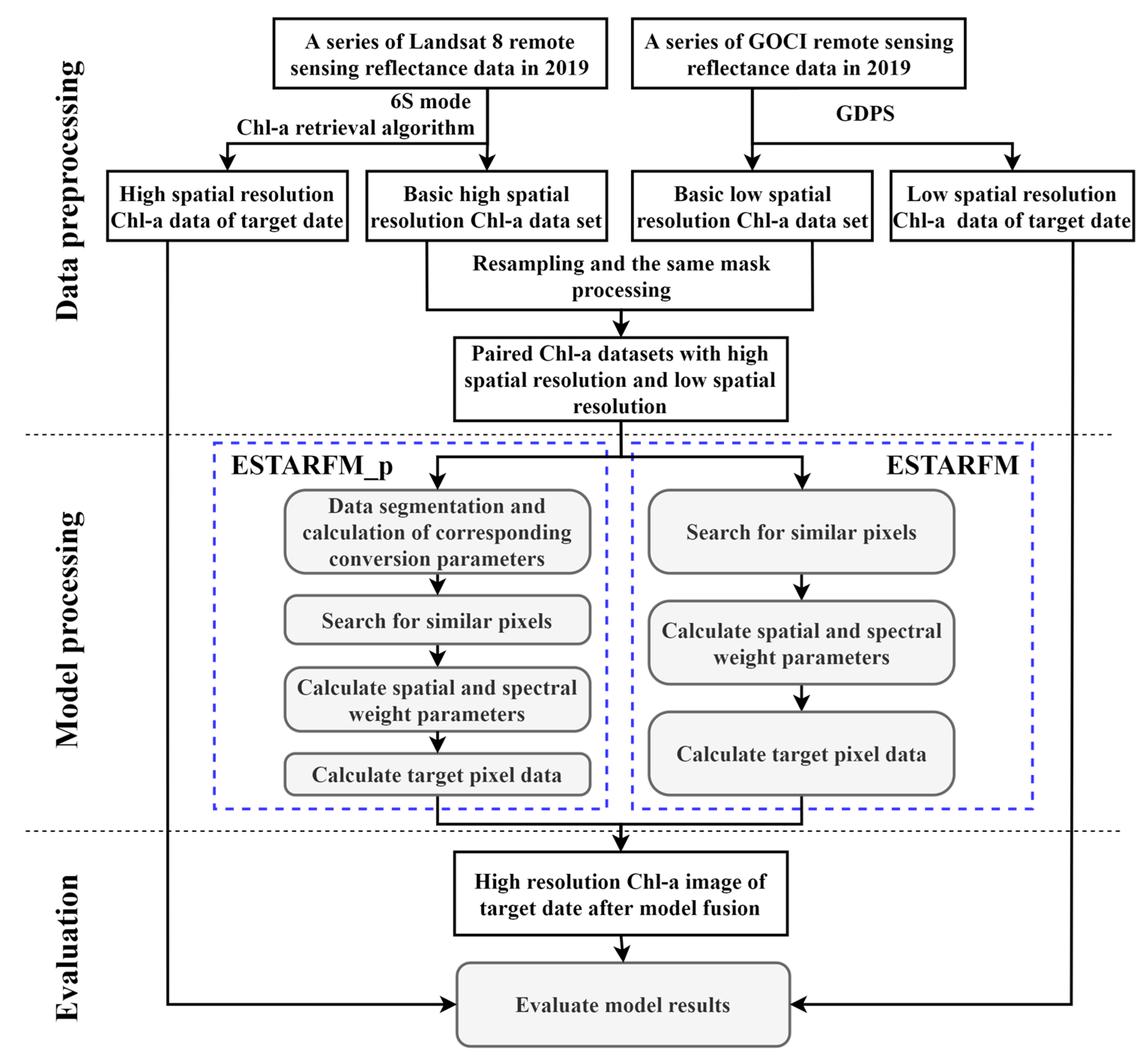
2.3. Methodology
2.4. Data Preprocessing
2.5. ESTARFM Fusion Model
2.6. ESTARFM_p Fusion Model
2.7. Evaluation
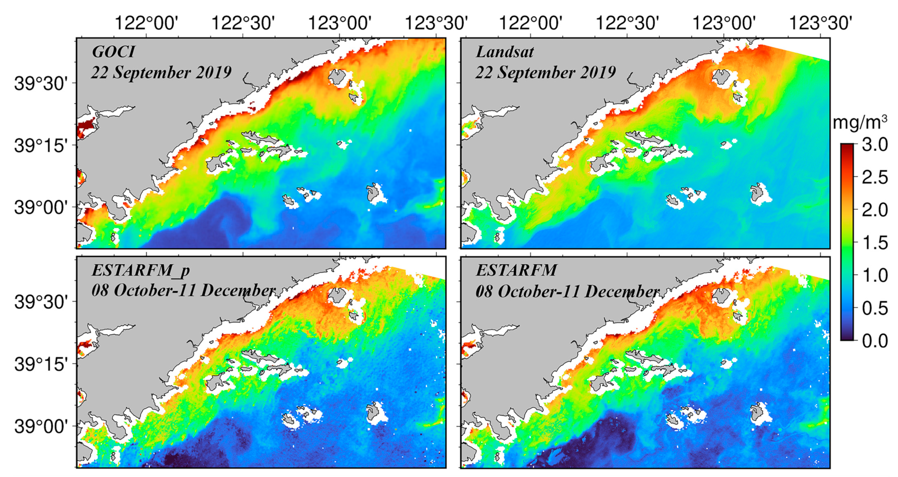
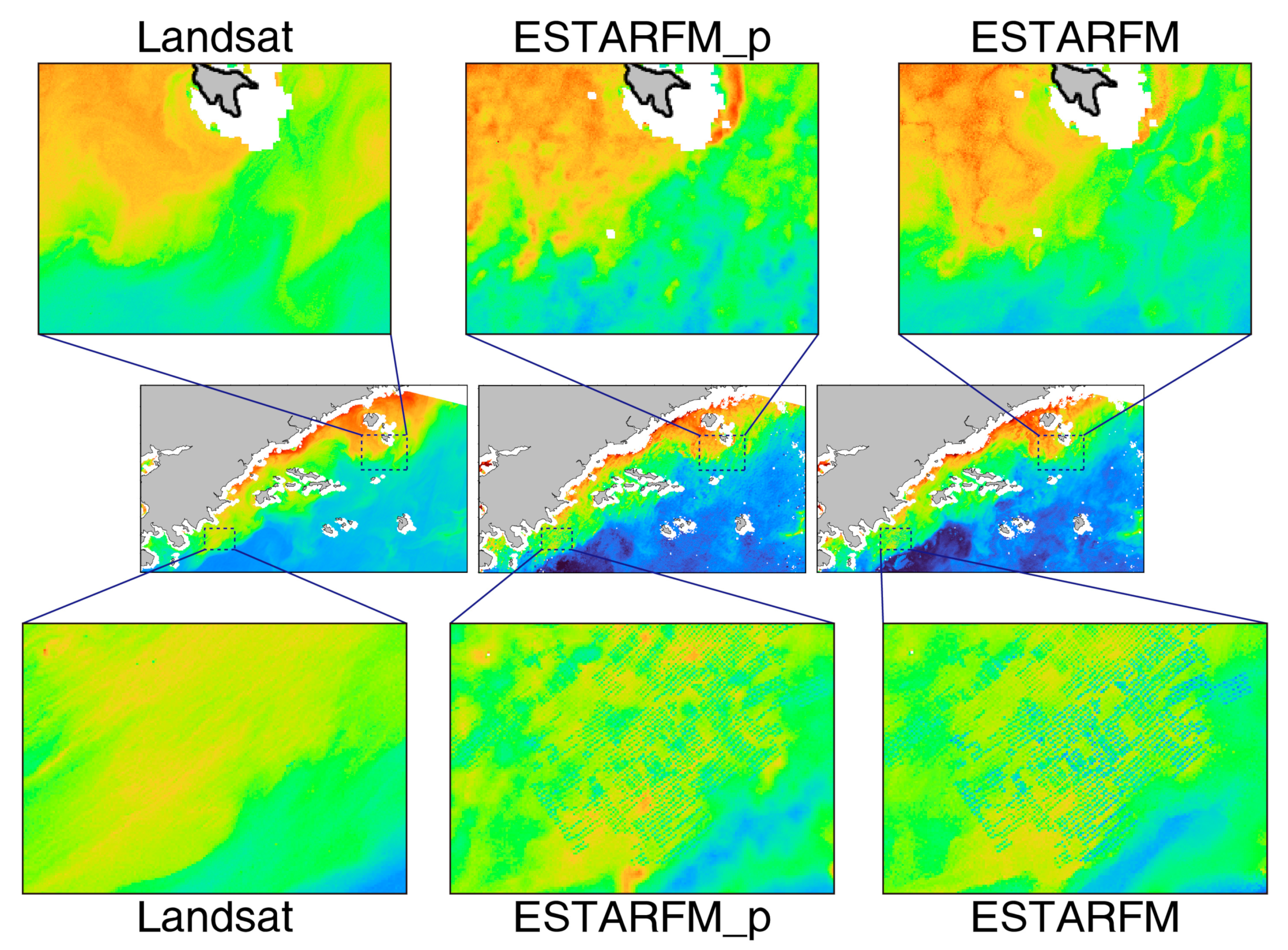
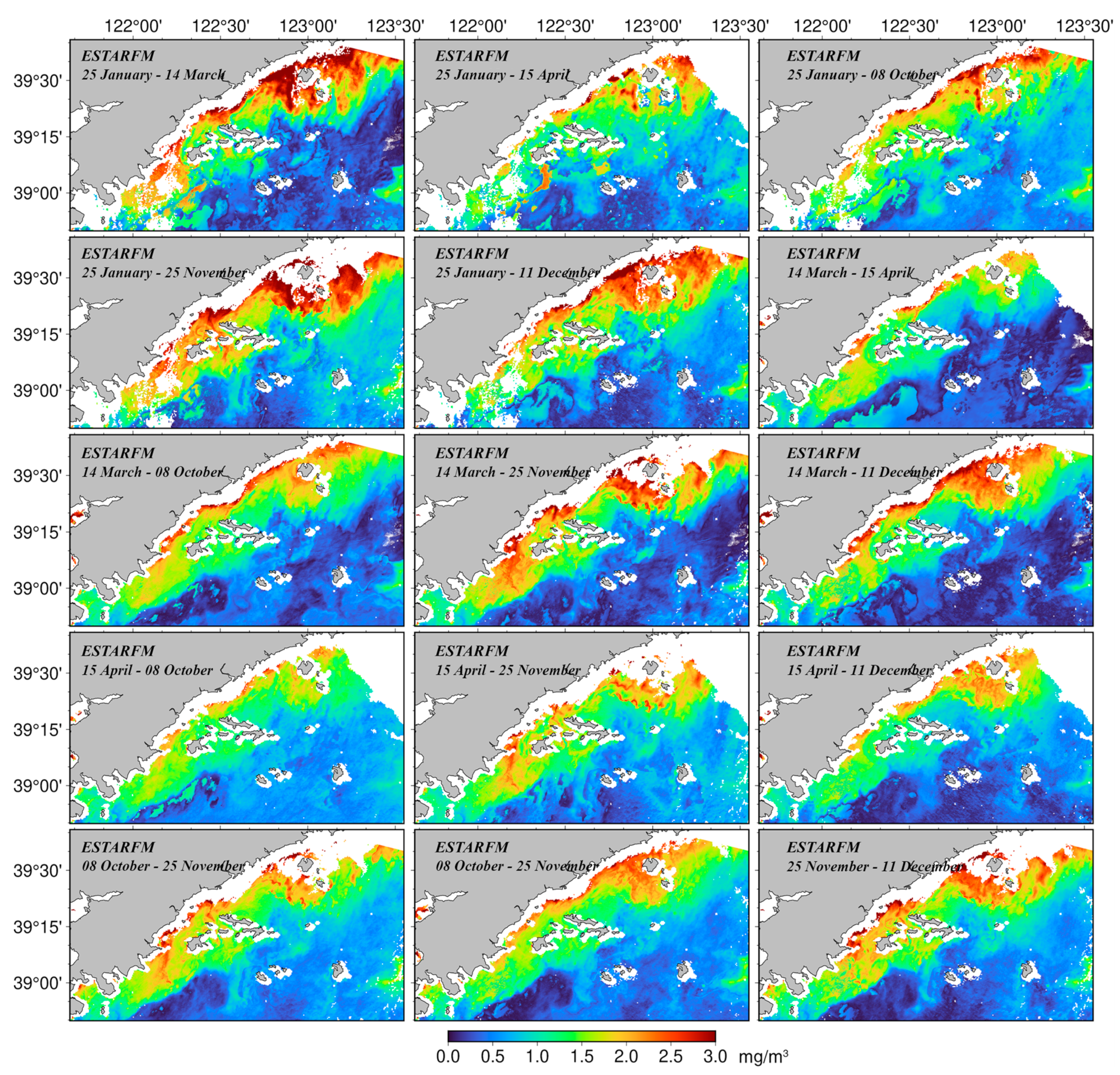
3. Results
4. Discussion
4.1. The Impact of Limited Input Data on Model Results
4.2. The Effect of the Temporal Distance between the Input and the Target on the Model Results
4.3. Comparison of Model Applicability
4.4. Limitations of the Models
5. Conclusions
Author Contributions
Funding
Data Availability Statement
Acknowledgments
Conflicts of Interest
References
- Price, J.C. How unique are spectral signature? Remote Sens. Environ. 1994, 49, 181–186. [Google Scholar] [CrossRef]
- Masek, J.G.; Huang, C.; Wolfe, R.; Cohen, W.; Hall, F.; Kutler, J.; Nelson, P. North American forest disturbance mapped from a decadal Landsat record. Remote Sens. Environ. 2008, 112, 2914–2926. [Google Scholar] [CrossRef]
- Yue, L.; Shen, H.; Li, J.; Yuan, Q.; Zhang, H.; Zhang, L. Image super-resolution: The techniques, applications, and future. Signal Process. 2016, 128, 389–408. [Google Scholar] [CrossRef]
- Yang, J.; Wright, J.; Huang, T.S.; Ma, Y. Image super-resolution via sparse representation. IEEE Trans. Image Process. 2010, 19, 2861–2873. [Google Scholar] [CrossRef]
- Hui, Z.; Li, J.; Gao, X.; Wang, X. Progressive perception-oriented network for single image super-resolution. Inform. Sci. 2021, 546, 769–786. [Google Scholar] [CrossRef]
- Zhang, H.; Yang, Z.; Zhang, L.; Shen, H. Super-Resolution Reconstruction for Multi-Angle Remote Sensing Images Considering Resolution Differences. Remote Sens. 2014, 6, 637–657. [Google Scholar] [CrossRef]
- Fisher, J. High spatial resolution sea surface climatology from Landsat thermal infrared data. Remote Sens. Environ. 2004, 90, 293–307. [Google Scholar] [CrossRef]
- Miskin, J.; Mackay, D. Ensemble Learning for Blind Image Separation and Deconvolution. In Advances in Independent Component Analysis; Springer: London, UK, 2000. [Google Scholar]
- Takeda, H.; Farsiu, S.; Milanfar, P. Kernel Regression for Image Processing and Reconstruction. IEEE T. Image Process. 2007, 16, 349–366. [Google Scholar] [CrossRef]
- Dong, C.; Loy, C.C.; He, K.; Tang, X. Image Super-Resolution Using Deep Convolutional Networks. IEEE T. Pattern Anal. 2016, 38, 295–307. [Google Scholar] [CrossRef]
- Trinh, D.; Luong, M.; Dibos, F.; Rocchisani, J.; Pham, C.; Nguyen, T.Q. Novel Example-Based Method for Super-Resolution and Denoising of Medical Images. IEEE T. Image Process. 2014, 23, 1882–1895. [Google Scholar] [CrossRef] [PubMed]
- Saharia, C.; Ho, J.; Chan, W.; Salimans, T.; Fleet, D.J.; Norouzi, M. Image Super-Resolution via Iterative Refinement. arxiv 2021, arXiv:2104.07636. [Google Scholar] [CrossRef]
- Guo, S.; Sun, B.; Zhang, H.K.; Liu, J.; Chen, J.; Wang, J.; Jiang, X.; Yang, Y. MODIS ocean color product downscaling via spatio-temporal fusion and regression: The case of chlorophyll-a in coastal waters. Int. J. Appl. Earth Obs. 2018, 73, 340–361. [Google Scholar] [CrossRef]
- Yocky, D.A. Multiresolution wavelet decomposition image merger of Landsat Thematic Mapper and SPOT panchromatic data. Photogramm. Eng. Remote Sens. 1996, 62, 1067–1074. [Google Scholar]
- Nunez, J.; Otazu, X.; Fors, O.; Prades, A.; Pala, V.; Arbiol, R. Multiresolution-based image fusion with additive wavelet decomposition. IEEE T. Geosci. Remote 1999, 37, 1204–1211. [Google Scholar] [CrossRef]
- Zhang, H.K.; Huang, B.; Zhang, M.; Cao, K.; Yu, L. A generalization of spatial and temporal fusion methods for remotely sensed surface parameters. Int. J. Remote Sens. 2015, 36, 4411–4445. [Google Scholar] [CrossRef]
- Gao, F.; Masek, J.; Schwaller, M.; Hall, F. On the blending of the Landsat and MODIS surface reflectance: Predicting daily Landsat surface reflectance. IEEE T. Geosci. Remote 2006, 44, 2207–2218. [Google Scholar]
- Hilker, T.; Wulder, M.A.; Coops, N.C.; Linke, J.; McDermid, G.; Masek, J.G.; Gao, F.; White, J.C. A new data fusion model for high spatial- and temporal-resolution mapping of forest disturbance based on Landsat and MODIS. Remote Sens. Environ. 2009, 113, 1613–1627. [Google Scholar] [CrossRef]
- Zhang, B.; Zhang, L.; Xie, D.; Yin, X.; Liu, C.; Liu, G. Application of Synthetic NDVI Time Series Blended from Landsat and MODIS Data for Grassland Biomass Estimation. Remote Sens. 2016, 8, 10. [Google Scholar] [CrossRef]
- Gao, F.; Anderson, M.C.; Zhang, X.; Yang, Z.; Alfieri, J.G.; Kustas, W.P.; Mueller, R.; Johnson, D.M.; Prueger, J.H. Toward mapping crop progress at field scales through fusion of Landsat and MODIS imagery. Remote Sens. Environ. 2017, 188, 9–25. [Google Scholar] [CrossRef]
- Zhu, X.; Chen, J.; Gao, F.; Chen, X.; Masek, J.G. An enhanced spatial and temporal adaptive reflectance fusion model for complex heterogeneous regions. Remote Sens. Environ. 2010, 114, 2610–2623. [Google Scholar] [CrossRef]
- Huang, B.; Zhang, H. Spatio-temporal reflectance fusion via unmixing: Accounting for both phenological and land-cover changes. Int. J. Remote Sens. 2014, 35, 6213–6233. [Google Scholar] [CrossRef]
- Bai, L.; Cai, J.; Liu, Y.; Chen, H.; Zhang, B.; Huang, L. Responses of field evapotranspiration to the changes of cropping pattern and groundwater depth in large irrigation district of Yellow River basin. Agr. Water Manag. 2017, 188, 1–11. [Google Scholar] [CrossRef]
- Pan, Y.; Shen, F.; Wei, X. Fusion of Landsat-8/OLI and GOCI Data for Hourly Mapping of Suspended Particulate Matter at High Spatial Resolution: A Case Study in the Yangtze (Changjiang) Estuary. Remote Sens. 2018, 10, 158. [Google Scholar] [CrossRef]
- Honeywill, C.; Paterson, D.M.; Hagerthey, S.E. Determination of microphytobenthic biomass using pulse-amplitude modulated minimum fluorescence. Eur. J. Phycol. 2002, 37, 485–492. [Google Scholar] [CrossRef]
- Gao, J.; Shi, H.; Zang, J.; Liu, Y. Mechanism analysis on the mitigation of harbor resonance by periodic undulating topography. Ocean Eng. 2023, 281, 114923. [Google Scholar] [CrossRef]
- Gao, J.; Ma, X.; Dong, G.; Chen, H.; Liu, Q.; Zang, J. Investigation on the effects of Bragg reflection on harbor oscillations. Coastal Eng. 2021, 170, 103977. [Google Scholar] [CrossRef]
- Gernez, P.; Doxaran, D.; Barillé, L. Shellfish Aquaculture from Space: Potential of Sentinel2 to Monitor Tide-Driven Changes in Turbidity, Chlorophyll Concentration and Oyster Physiological Response at the Scale of an Oyster Farm. Front. Mar. Sci. 2017, 4, 137. [Google Scholar] [CrossRef]
- Harvey, E.T.; Kratzer, S.; Philipson, P. Satellite-based water quality monitoring for improved spatial and temporal retrieval of chlorophyll-a in coastal waters. Remote Sens. Environ. 2015, 158, 417–430. [Google Scholar] [CrossRef]
- Kahru, M.; Kudela, R.M.; Lorenzo, E.D.; Manzano-Saraba, M.; Mitchell, B.G. Trends in the surface chlorophyll of the California Current: Merging data from multiple ocean color satellites. Deep Sea Res. Part II Top. Stud. Oceanogr. 2012, 77–80, 89–98. [Google Scholar] [CrossRef]
- Gregg, W.W.; Conkright, M.E. Global seasonal climatologies of ocean chlorophyll; blending in situ and satellite data for the Coastal Zone Color Scanner era. J. Geophys. Res. Ocean. 2001, 106, 2499–2515. [Google Scholar] [CrossRef]
- Wang, B.; Wang, X.; Zhan, R. Nutrient conditions in the Yellow Sea and the East China Sea. Estuar. Coast. Shelf Sci. 2003, 58, 127–136. [Google Scholar] [CrossRef]
- Zhang, H.; Shi, X.; Zhang, C.; Wang, L.I.S. Distribution Features of Nutrients Structure and Nutrient Limitation in the North of Yellow Sea. Period. Ocean. Univ. China 2009, 39, 8. [Google Scholar]
- Li, Y.W.; Hu, Y.Y.; Chen, S. Distribution and influence factors of nutrients in the North Yellow Sea in Summer and Autumn. China Environ. Sci. 2013, 33, 1060–1067. [Google Scholar]
- Wu, Y.; Zhang, J.; Zhao, L.; Chen, C. Spatiotemporal Characteristics of Nitrogen and Phosphorus and Its Influencing Processes in the Yellow Sea. J. Tianjin Univ. Sci. Technol. 2021, 36, 30–40. [Google Scholar]
- Ahn, J.; Park, Y.; Ryu, J.; Lee, B.; Oh, I.S. Development of atmospheric correction algorithm for Geostationary Ocean Color Imager (GOCI). Ocean. Sci. J. 2012, 47, 247–259. [Google Scholar] [CrossRef]
- Gordon, H.R.; Wang, M. Retrieval of water-leaving radiance and aerosol optical thickness over the oceans with SeaWiFS: A preliminary algorithm. Appl. Opt. 1994, 33, 443–452. [Google Scholar] [CrossRef]
- Gordon, H.R.; Wang, M. Influence of oceanic whitecaps on atmospheric correction of ocean-color sensors. Appl. Opt. 1994, 33, 7754–7763. [Google Scholar] [CrossRef]
- Kotchenova, S.Y.; Vermote, E.F.; Matarrese, R.; Klemm, J.F.J. Validation of a vector version of the 6S radiative transfer code for atmospheric correction of satellite data. Part I: Path radiance. Appl. Opt. 2006, 45, 6762–6774. [Google Scholar] [CrossRef]
- Kotchenova, S.Y.; Vermote, E.F. Validation of a vector version of the 6S radiative transfer code for atmospheric correction of satellite data. Part II. Homogeneous Lambertian and anisotropic surfaces. Appl. Opt. 2007, 46, 4455–4464. [Google Scholar] [CrossRef] [PubMed]


| Date | Platform/Sensor | Time |
|---|---|---|
| 25 January 2019 | Landsat/GOCI | 10:30 |
| 14 March 2019 | Landsat/GOCI | 10:30 |
| 15 April 2019 | Landsat/GOCI | 10:30 |
| 22 September 2019 | Landsat/GOCI | 10:30 |
| 8 October 2019 | Landsat/GOCI | 10:30 |
| 25 November 2019 | Landsat/GOCI | 10:30 |
| 11 December 2019 | Landsat/GOCI | 10:30 |
| a0 | a1 | a2 | a3 | a4 | |
|---|---|---|---|---|---|
| OC3 | 0.2412 | −2.0546 | 1.1776 | −0.5538 | −0.4570 |
| OC3g | 0.0831 | −1.9941 | 0.5629 | 0.2944 | −0.5458 |
| Date | 25 Jan | 14 Mar | 15 Apr | 8 Oct | 25 Nov |
|---|---|---|---|---|---|
| 14 March | 14 March–25 January | ||||
| 15 April | 15 April–25 January | 15 April–14 March | |||
| 8 October | 8 October–25 January | 8 October–14 March | 8 October–15 April | ||
| 25 November | 25 November–25 January | 25 November–14 March | 25 November–15 April | 25 November–8 October | |
| 11 December | 11 December–25 January | 11 December–14 March | 11 December–15 April | 11 December–8 October | 11 December–25 November |
Disclaimer/Publisher’s Note: The statements, opinions and data contained in all publications are solely those of the individual author(s) and contributor(s) and not of MDPI and/or the editor(s). MDPI and/or the editor(s) disclaim responsibility for any injury to people or property resulting from any ideas, methods, instructions or products referred to in the content. |
© 2023 by the authors. Licensee MDPI, Basel, Switzerland. This article is an open access article distributed under the terms and conditions of the Creative Commons Attribution (CC BY) license (https://creativecommons.org/licenses/by/4.0/).
Share and Cite
Meng, Q.; Song, J.; Fu, Y.; Cai, Y.; Guo, J.; Liu, M.; Jiang, X. Downscaling of Oceanic Chlorophyll-a with a Spatiotemporal Fusion Model: A Case Study on the North Coast of the Yellow Sea. Water 2023, 15, 3566. https://doi.org/10.3390/w15203566
Meng Q, Song J, Fu Y, Cai Y, Guo J, Liu M, Jiang X. Downscaling of Oceanic Chlorophyll-a with a Spatiotemporal Fusion Model: A Case Study on the North Coast of the Yellow Sea. Water. 2023; 15(20):3566. https://doi.org/10.3390/w15203566
Chicago/Turabian StyleMeng, Qingdian, Jun Song, Yanzhao Fu, Yu Cai, Junru Guo, Ming Liu, and Xiaoyi Jiang. 2023. "Downscaling of Oceanic Chlorophyll-a with a Spatiotemporal Fusion Model: A Case Study on the North Coast of the Yellow Sea" Water 15, no. 20: 3566. https://doi.org/10.3390/w15203566
APA StyleMeng, Q., Song, J., Fu, Y., Cai, Y., Guo, J., Liu, M., & Jiang, X. (2023). Downscaling of Oceanic Chlorophyll-a with a Spatiotemporal Fusion Model: A Case Study on the North Coast of the Yellow Sea. Water, 15(20), 3566. https://doi.org/10.3390/w15203566