Article

Empowering Greenhouse Cultivation: Dynamic Factors and Machine Learning Unite for Advanced Microclimate Prediction

Department of Bioenvironmental Systems Engineering, National Taiwan University, Taipei 10617, Taiwan
*
Author to whom correspondence should be addressed.
Water 2023, 15(20), 3548; https://doi.org/10.3390/w15203548
Submission received: 13 September 2023 / Revised: 3 October 2023 / Accepted: 8 October 2023 / Published: 11 October 2023

Abstract

:
Climate change has led to more frequent extreme weather events such as heatwaves, droughts, and storms, which significantly impact agriculture, causing crop damage. Greenhouse cultivation not only provides a manageable environment that protects crops from external weather conditions and pests but also requires precise microclimate control. However, greenhouse microclimates are complex since various heat transfer mechanisms would be difficult to model properly. This study proposes an innovative hybrid model (DF-RF-ANN), which seamlessly fuses three components: the dynamic factor (DF) model to extract unobserved factors, the random forest (RF) to identify key input factors, and a backpropagation neural network (BPNN) to predict greenhouse microclimate, including internal temperature, relative humidity, photosynthetically active radiation, and carbon dioxide. The proposed model utilized gridded meteorological big data and was applied to a greenhouse in Taichung, Taiwan. Two comparative models were configured using the BPNN and the Long short-term memory neural network (LSTM). The results demonstrate that DF-RF-ANN effectively captures the trends of the observations and generates predictions much closer to the observations compared to LSTM and BPNN. The proposed DF-RF-ANN model hits a milestone in multi-horizon and multi-factor microclimate predictions and offers a cost-effective and easily accessible approach. This approach could be particularly beneficial for small-scale farmers to make the best use of resources under extreme climatic events for contributing to sustainable development goals (SDGs) and the transition towards a green economy.

1. Introduction

1.1. Background

Climate change has caused devastating disasters in various regions worldwide, such as Cyclone Idai, fatal heatwaves in India and Europe, and flooding in southeast Asia [1]. The Institute for Economics & Peace (IEP), an international think tank, foresees that those affected by the changing climate will need to face the reality that climate change is causing the displacement of people, poverty, and food insecurity. In addition to its impact on water resources management, climate change also raises the possibility of environmental and socioeconomic dislocations. The regional impact of climate change necessitates tailoring adaptation measures to local climatic, hydrological, and social conditions [2,3]. With the advent of climate change and unpredictable weather events, greenhouse cultivation has emerged as a crucial tool to stabilize crop prices and ensure food security through controlled environments. Precision agriculture has gained substantial momentum, finding application within greenhouse settings to effectively address and mitigate the challenges posed by climate change and natural disasters. Advancements in greenhouse technology, spanning both hardware and software innovations like the Internet of Things (IoT), cloud-based servers, and machine learning, have made the realization of precision agriculture in greenhouses more achievable. Greenhouses provide a controlled environment, incorporating precise regulation of factors such as temperature and humidity, which can significantly bolster agricultural production. However, it is crucial to recognize the intricacy of controlling the microclimate within greenhouses, characterized by highly nonlinear and dynamic systems. Consequently, the development of microclimate prediction models becomes paramount for farmers. Such models empower proactive greenhouse management, ensuring the creation of an optimal environment for crops and, consequently, elevating overall agricultural productivity.
Nevertheless, predicting and managing the microclimates within greenhouses can be very challenging due to the intricate heat transfer dynamics in such settings. The environmental management of greenhouses is essential for cultivating crops in favorable microclimates [4]. Several factors can influence greenhouse microclimates, such as temperature (Temp), relative humidity (RH), photosynthetically active radiation (PAR), and carbon dioxide (CO2). For instance, maintaining appropriate RH levels is crucial for crop growth, as it can influence both crop quality and the cost of dehumidification [5,6]. Manual cooling is often necessary to regulate Temp within the greenhouse to ensure optimal conditions for crop physiology [7]. Besides, proper ventilation is critical to temperature control within greenhouses, as greenhouse operations can directly influence the heat transfer between internal and external environments [8]. Photosynthesis serves as the fundamental driver of crop growth and quality, influenced by various factors. Different plants require different levels of PAR, and, on average, a 1% increase in PAR can lead to a 0.5–1% increase in yield for most crops [9]. CO2 is crucial for crop photosynthesis and can significantly impact crop growth. Therefore, monitoring CO2 concentration is essential during crop cultivation. Previous studies have demonstrated that increasing the concentration of CO2 can improve crop yields [10,11].
Accurately predicting greenhouse microclimates is crucial but can be challenging due to the complex mass exchanges related to internal elements like plants and soil, manual control like windows, roller blinds, and fans, and meteorological factors like solar radiation, temperature, and evaporation. Greenhouse models can be categorized into two primary groups: physically-based and data-driven models. Physically based models can offer physical laws with reasonable justifications. However, heat and mass transfers in the real world are highly complex, and their predictions often require unmeasurable parameters such as photosynthesis rate, heat flux density, and heat transfer coefficients [12,13]. If these unmeasurable parameters cannot be estimated properly, it could be challenging to accurately predict heat and mass transfers.

1.2. Related Works

Data-driven techniques such as artificial neural networks (ANNs) and machine learning are currently applied in numerous fields. For instance, Naïve Bayes classifiers have demonstrated remarkable classification capabilities in the context of Cardiovascular diseases [14], whereas K-Nearest Neighbor algorithms have showcased impressive effectiveness in predicting movie market potential [15]. Moreover, innovative hybrid machine-learning techniques have consistently surpassed traditional approaches. For instance, the combination of LSTM with attention mechanisms has excelled in solving multivariate time series problems [16], and BPNN, in conjunction with the three-way decisions (TWD) framework, has exhibited outstanding performance in long-term prediction [17]. Furthermore, deep convolutional neural networks have been successfully employed for protein classification and protein family prediction [18].
ANNs are utilized in hydrological studies, including urban flood forecasting [19,20], groundwater level prediction [21], rainfall-runoff prediction [22], water quality modeling [23,24], and microclimate prediction [25]. ANNs are becoming increasingly popular in predicting greenhouse microclimates as they can quickly and accurately analyze large amounts of data [26,27]. Furthermore, when sensors are deployed within greenhouses, ANNs have demonstrated their ability to deliver accurate microclimate predictions [28]. The hybridization of machine learning methods has gained popularity and demonstrated notable improvements in prediction accuracy [29]. One prominent advantage of ANNs is their ability to account for the intricate interactions among various environmental factors, such as temperature, humidity, and light intensity, which can affect microclimate conditions within the greenhouse.
It has been observed that the prediction accuracy of ANNs for greenhouse microclimates can be improved by incorporating other statistical and machine-learning techniques. One such technique is the dynamic factor (DF) model, which is a useful linear approach for analyzing multivariate time series data with time-varying dynamics and identifying common patterns among multiple time series [30]. The DF model has been applied in diverse fields, including economic prediction [31,32], psychological assessment [33], and PM2.5 factor analysis [34]. Besides, a DF-based model was also utilized for the analysis and prediction of survey-based consumer confidence [35]. Hybrid models that combine ANN and DF have also been developed for various applications, such as evaporation prediction [36] and performance comparison [37]. However, the challenge of selecting appropriate input factors to improve prediction accuracy persists. The random forest (RF) is a powerful machine-learning technique capable of identifying key factors and reducing dimensionality [38]. It has been widely used to solve problems in various environmental domains, including photovoltaic power generation forecasting [39], spatial prediction of gully erosion susceptibility [40], and predicting blast-induced air overpressure [41]. Furthermore, RF has recently been applied to predict CO2 emissions resulting from road transport, demonstrating excellent performance [42].

1.3. Proposed Solution

Numerous studies have focused on advanced machine learning models for microclimate prediction, yet few have explored the integration of linear models, which could offer valuable insights into microclimate prediction [43]. Furthermore, many predictive methods rely on IoT sensors, incurring substantial maintenance costs for farmers [28]. Additionally, a notable portion of research lacks explanations for the selection of input features [28,29]. To tackle these challenges, this study aims to propose a novel hybrid model (DF-RF-ANN) that effectively captures stochastic and deterministic features from complex heterogeneous datasets to accurately predict greenhouse microclimate. The DF-RF-ANN model seamlessly fuses DF for filtering unobserved factors, RF for selecting key factors, and ANN for predicting one- and two-hour-ahead microclimates. These predictions can assist farmers in adequately regulating greenhouse facilities such as windows, roller blinds, and fans to create an optimal environment for crop cultivation. The integration of linear (DF) and non-linear (RF, back propagation neural network (BPNN)) techniques is anticipated to improve prediction accuracy and reliability. Besides, we leverage data provided by Taiwan’s Central Weather Administration (CWA), which not only lessens the reliance on IoT sensors but also alleviates the burden on farmers. This study also compares the prediction performance of DF-RF-ANN with BPNN and a long short-term memory neural network (LSTM). The results can be provided to farmers for managing greenhouse operations two hours in advance at a low cost. The findings of this study can aid farmers in managing cost-effective greenhouse management by providing microclimate predictions for the next two hours.

2. Materials and Methods

2.1. Study Area and Materials

A plastic film greenhouse measuring 12 m in length and 5 m in width, with varying heights of 4 m (highest point) and 3 m (lowest point), located in Taichung, Taiwan, and managed by the Taiwan Agricultural Research Institute (TARI) formed the case study (Figure 1). Field experiments with cherry tomatoes were carried out in the greenhouse over one and a half years, from 1 April 2020 to 13 July 2021. The data for this study was divided into approximately 60% for training, 20% for validation, and 20% for testing purposes. Due to the significant heterogeneity in various input data types, we employed the min-max normalization technique for data preprocessing. This procedure effectively rescales the data to fall within [0, 1]. During the period, both internal and external data were collected. Internal data were measured by an Internet of Things (IoT) sensor module at a 10-min interval, including four crucial factors, namely Temp, RH, PAR, and CO2, all of which significantly impact the growth of cherry tomatoes. We utilized the internal data for model calibration as one of our objectives was to generate accurate 2-h-ahead predictions of internal microclimate without relying on IoT. External data were generated by the space and time multiscale analysis system and weather research and forecasting model (STMAS-WRF) of Taiwan’s Central Weather Administration (CWA). STMAS extracts weather-related features, while WRF provides gridded weather forecast data [44]. With a resolution of 3 × 3 km2, the STMAS-WRF model generates hourly forecasts of multiple climate factors, such as surface temperature (TSF, unit: K), dew point temperature (DSF in units of K), relative humidity (RH in units of %), short-wave radiation (SWI in units of W/m2), long wave radiation (LWO in units of W/m2), surface pressure (PSF in units of hPa), atmospheric pressure (SLP in units of hPa), and vapor pressure deficit (VPD in units of hPa). The TARI greenhouse is equipped with six controllers to regulate the environment: roof roller shades on both sides, left roller shade, right roller shade, front roller shade, rear roller shade, and inner fans. It takes 103.6 ± 12.0 s to open all the rollers, leading to a 1 °C reduction in Temp.

2.2. Method

This study aims to predict the greenhouse internal microclimate solely based on gridded climate forecasts provided by the CWA, thereby eliminating the need for farmers to install or maintain IoT devices and reducing greenhouse cultivation costs. To accomplish this goal, we develop a novel model (DF-RF-ANN) that seamlessly integrates DF, RF, and ANN to capture the trends of climate factors, identify proper climate factors, and predict internal microclimate, respectively (Figure 2). Comparative models include LSTM and BPNN. The methods used are briefly introduced in the following section.

2.2.1. Random Forest (RF)

RF is a powerful machine-learning technique for performing feature extraction and dimensionality reduction [45]. It excels at feature selection by identifying the most significant input factors that impact the output. RF combines tree predictors, where each tree is independent and follows the same distribution within the forest [46]. Each tree uses the bootstrapped technique to sample the data. RF can reduce the number of input factors by utilizing subsets with fewer factors than the total number of input factors. In classification problems, RF receives a class vote from each tree and subsequently applies the majority voting criterion to classify each sample [47]. RF is known for its stability, shorter training time, and superior performance. This method has been utilized in various research areas, including feature selection from the penicillin fermentation process [48]. This study uses RF to select key factors based on their importance values.

2.2.2. Artificial Neural Network (ANN)

ANNs are potent techniques and valuable tools for modeling complex systems, such as classification, prediction, and estimation. One of the primary advantages of ANNs is their capability to predict based on patterns and relationships in input factors, with a wide range of applications, including image and speech recognition [49,50] and hydrological and environmental forecasting [51,52].
This study uses two types of ANN (BPNN and LSTM) to predict the greenhouse microclimate. The proposed DF-RF-ANN model employs BPNN, configured with five hidden layers because it can deliver excellent prediction performance when multiple input factors are involved. BPNN and LSTM constitute two comparative models.

Backpropagation Neural Network (BPNN)

BPNN, developed by Rumelhart and Williams in 1985 [53], is a classic and popular neural network for prediction and estimation in various fields. BPNN is a feed-forward neural network comprising input, hidden, and output layers (Figure 2). In this study, BPNN was trained to minimize the global error for fitting the problem using the training datasets. To avoid gradient vanishing problems and extract non-linear features from input factors, we used the Rectified Linear Unit (ReLU, Equation (1)) as an activation function. After training and building the model, it was validated and tested with additional datasets. Furthermore, BPNN functions as a predictor and serves as a base component of the proposed hybrid model.
y = max(y, 0) with y = f(x)
where y = f(x) is a linear function.

Long Short-Term Memory Neural Network (LSTM)

LSTM has gained widespread popularity in recent years as it can overcome the limitations of traditional recurrent neural networks (RNNs) and has demonstrated good performance in hydrological fields [54,55]. In contrast to traditional RNNs, which have short-term memories but lack long-term ones, LSTM contains a memory cell and three gates: input, output, and forget gates. These gates enable LSTM to address the issue of forgetting important information by controlling how much information is used (input gate), removed (forget gate), and retained in the memory cell. Additionally, the output gate determines the information that needs to be generated as output.

2.2.3. Dynamic Factor (DF) Model

The DF model is used for multivariate time-series analysis and is commonly adopted to identify trends in economic variables. This method explains the covariance structure of a set of observed variables using a small number of latent variables known as “factors”. These factors are assumed to be influenced by unobserved processes that capture the underlying patterns and trends in the data. The formula for DF is presented below.
y t = f t + u t
where yt denotes observed data; ⋀ denotes factor loadings; ft denotes the unobserved factors; and ut denotes an idiosyncratic component or error.
Several studies have demonstrated that the Dynamic Factor (DF) model has the capability to amalgamate data of different frequencies into a latent coincident index [56]. This is the rationale behind our attempt to integrate this method for uncovering unobserved factors. This study used DF to generate unobserved factors to enhance prediction accuracy, which were subsequently fed into BPNN. For the DF procedure, the Statsmodels package (version: 0.13.2) was implemented [57].

2.2.4. Hybrid Model (DF-RF-ANN)

The proposed model for predicting greenhouse internal microclimate based on the external data from the STMAS-WRF is a hybrid approach that combines DF, RF, and BPNN, as depicted in Figure 2. Since BPNN does not consider time series patterns, DF can be used to extract the trend information of input factors and provide time-varying unobserved factors as inputs to BPNN. Moreover, an excessive number of input factors can lead to model inaccuracy due to excessive noise and overfitting. Therefore, RF is utilized to select the key input factors for each output of BPNN from among the 48–50 input candidates provided in this study (Figure 2). The construction of DF-RF-ANN involves three main steps, which are addressed as follows.
Step 1: Utilize the DF model to uncover unobserved factors.
Step 2: Utilize the RF model to identify important factors from the unobserved factors and climate factors.
Step 3: Utilize the important factors as inputs to train BPNN for producing T + 1 and T + 2 predictions.
The hyperparameter settings for the DF-RF-ANN model can be found in Appendix A, and the selection of input factors is detailed in Table 1. We opted for the ReLU as our activation function to address the vanishing gradient issue. Following experimentation with various configurations, we employed six hidden layers in our neural networks.
Predicting greenhouse internal microclimate is a complex task when using STMAS-WRF data, which are forecasted external climate data obtained from the CWA. Consequently, there were two major sources of noise. The first source was that the STMAS-WRF data were forecasts rather than actual data collected from climate stations. The second source was the complex and non-linear relationship between external and internal microclimates. These two sources of noise could accumulate during the prediction process. Therefore, we tested various hybrid models to reduce these errors and achieve better performance.

2.3. Evaluation of Model Performance

This study used the coefficient of determination (R2) and the mean absolute error (MAE) as the performance indicators to evaluate the constructed models.
Coefficient of Determination
R 2 = i = 1 N y i y ¯ o i o ¯ i = 1 N y i y ¯ 2 i = 1 N o i o ¯ 2 2
Mean Absolute Error
M A E = 1 N i = 1 N y i o i
where yi is the output value of the model, oi is the observation value,    y ¯  is the average of output values,  o ¯    is the average of observation values, and N is the number of data.
R2 is an indicator for assessing the linearity between predicted and observed values. MAE is used to assess prediction accuracy. A higher (lower) R2 (MAE) value indicates that the model predicts more accurately.

3. Results and Discussion

The proposed DF-RF-ANN model that combines the advantages of RF, DF, and BPNN is constructed to predict greenhouse microclimate based on hourly climate forecasts (T + 1 up to T + 6) obtained from STMAT-WRF. These forecasts include surface temperature, vapor pressure deficit, dew point temperature, long-wave radiation, surface pressure, relative humidity, atmospheric pressure, and short-wave radiation. BPNN and LSTM are configured as two comparative models. The findings, results, and discussion are given below.

3.1. Unobserved Factors Derived from the DF Model

This study aims to extract unobserved factors from various climate factors. To achieve this, we created two distinct groups of climate factors: Group 1 comprised of TSF, DSF, and SWI, while Group 2 comprised RH and VPD. We sought to extract an unobserved factor (DFM 1) from Group 1 to enhance the prediction accuracy of Temp and PAR since elements in Group 1 are closely related to these variables. Another unobserved factor (DFM 2) was derived from Group 2 since the elements in this group have a more direct influence on plant physiology, which affects CO2 concentration. Therefore, DFM 2 is expected to significantly contribute to predictions of CO2 concentration.
Figure 3 illustrates the trends of two unobserved factors (DFM 1 and DFM 2) and four target factors (PAR, RH, Temp, and CO2). It can be observed that DFM 1 and DFM 2 exhibit similar behavior, but the valleys of DFM 1 are lower than those of DFM 2. Besides, DFM 1 shows an opposite trend to Temp and PAR, whereas DFM 2 shows a similar trend to CO2. This could be attributed to the fact that as VPD increases, leaf stomata tend to close, leading to reduced photosynthesis and CO2 uptake [58]. Furthermore, higher VPD leads to lower RH.

3.2. Factor Identification by RF

In this study, there were a total of 50 candidate factors (=8 × 6 + 2, comprising eight climate factors with 6-step-ahead forecasts from STMAT-WRF and two unobserved factors, DFM 1 and DFM 2). Due to the high number of input factors, which could potentially reduce the prediction performance of BPNN, we implemented RF to identify key factors by ranking their importance. Subsequently, we constructed BPNN with various input combinations to predict the internal microclimate, focusing on one output factor at a time. The results of RF are shown in Table 1.
The top ten factors identified by RF for predicting Temp, ranked in descending order of importance, are listed as follows: TSF T + 1, SWI T + 1, DFM1, SWI T + 2, TSF T + 2, LWO T + 1, LWO T + 2, VPD T + 1, LWO T + 4, and DFM2 (Table 1). It can be observed that TSF T + 1 (ranked first) is most strongly related to Temp. SWI is also significantly related to Temp. An example of the need to include SWI as an input factor in empirical temperature-index models can be found in Pellicciotti et al. (2005) [59]. Moreover, LWO can impact the heat balance, as suggested by Livingstone (1998) [60]. It is worth noting that VPD and DFM 2 are also ranked among the top ten factors. It is important to note that Model T1 produces a lower R2 value than Model T4, which excludes DFM 2, LWO, and VPD. This indicates that a model with too many input factors can cause a decrease in model performance. In this study, we constructed BPNN prediction models with different input combinations by removing low-ranking factors for each target climate factor (as shown in Table 1). When predicting Temp using BPNN with more than two input factors, it is observed that reducing the number of input factors leads to an increase in prediction performance (R2). This supports the idea that including too many input factors can result in poorer prediction performance. On the other hand, Model T5, with only two input factors, performs even worse than Model T4, with three input factors, indicating that the input information is insufficient for Model T5 and results in poorer predictions. Furthermore, the inclusion of DFM 1, which is significantly related to Temp, as an input factor helps improve prediction performance, as expected.
For predicting RH, the top 10 input factors obtained from RF, ranked in descending order of importance, are listed as follows: SWI T + 1; DFM 1; RH T + 1; VPD T + 1; SWI T + 6; LWO T + 1; DFM 2; LWO T + 2; RH T + 2; and LWO T + 5 (Table 1). Based on the input factors, Model R3 (with SWI, DFM 1, RH, and VPD) best predicted RH because it had the highest R2 value. SWI is a significant factor in predicting RH because it influences the amount of heat absorbed and radiated back into the atmosphere by the land surface, ultimately affecting humidity levels [61]. The second most crucial factor affecting RH is DFM 1, suggesting a hidden relationship between RH and the group of TSF, DSF, and SWI. Moreover, VPD can be calculated from Temp and RH [62], which explains why VPD is highly correlated with RH. It is noteworthy that DFM 2 is not included in Model R3, which may be due to the fact that DFM 2 is derived from RH and VPD and, therefore, has lower importance compared to RH and VPD.
The best-performing model for predicting PAR, which is closely linked to crop photosynthesis, is Model P2 (with nine input factors). The top-ranking input factors in Model P2, from high to low, are SWI T + 2, VPD T + 1, SWI T + 3, SWI T + 1, DFM 2, DFM 1, TSF T + 1, LWO T + 1, and SWI T + 4. It can be inferred that long- and short-wave radiation are significantly related to PAR. Besides, the inclusion of VPD and TSF in Model P2 is reasonable because PAR exhibits similar variation to these two factors [63]. Model P2 also incorporates DFM 1 and DFM 2, indicating that DF is meaningful and beneficial in this study. The process of photosynthesis is critical for crop growth and relies significantly on light intensity and CO2 concentration [64]. As a result, it is important to predict the CO2 concentration in the greenhouse. However, obtaining accurate CO2 concentration measurements without the use of IoT can be challenging due to the complex interactions within the greenhouse environment during crop cultivation. According to Table 1, Model C2 with seven input factors (VPD T + 1, DFM 2, TSF T + 1, SWI T + 1, SWI T + 6, DFM 1, and TSF T + 2) exhibits the best prediction performance for CO2 concentration. As mentioned earlier, CO2 is closely related to photosynthesis and, therefore, to factors that promote photosynthesis, such as SWI, TSF, and VPD. Furthermore, the inclusion of DFM 1 and DFM 2 in Model C2 highlights the significance of DF in predicting CO2 concentration.
Overall, the results shown in Table 1 indicate that incorporating DFM 1 as an input factor in BPNN models can enhance the prediction performance of Temp, RH, PAR, and CO2, while including DFM 2 can improve the prediction performance of PAR and CO2.

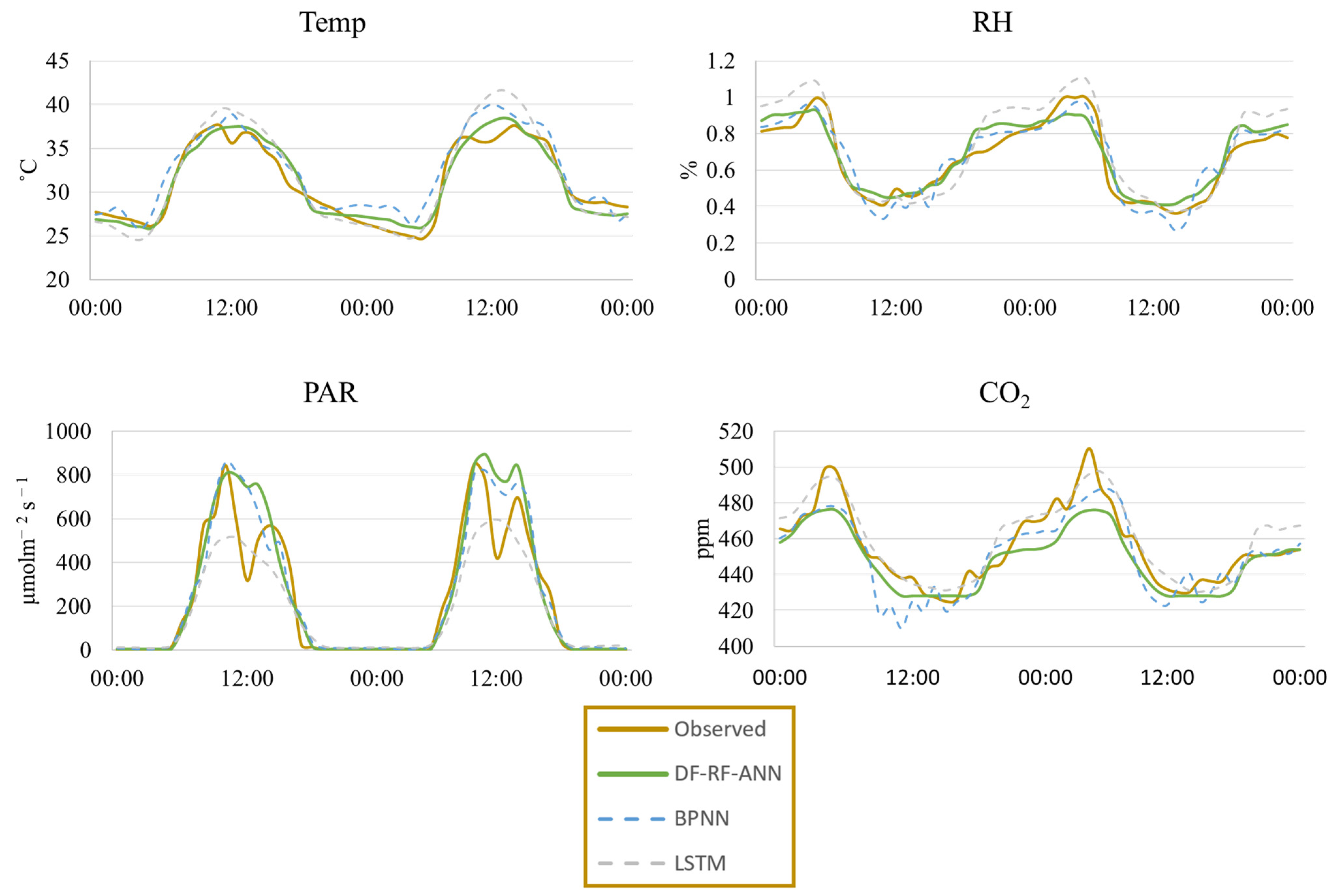
3.3. Model Comparison

The comparison outcomes of DF-RF-ANN, LSTM, and BPNN are presented in Table 2 as well as Figure 4. As shown in Table 2, LSTM outperforms BPNN with respect to R2 values, except in the case of PAR prediction. In terms of R2 and MAE, DF-RF-ANN surpasses both LSTM and BPNN. Particularly concerning Temp, employing just three input factors in DF-RF-ANN demonstrates enhancements of 7.69% over BPNN and 1.32% over LSTM. For RH, DF-RF-ANN elevates predictive accuracy by 22.51% and 9.54% compared to BPNN and LSTM, respectively. Regarding PAR, DF-RF-ANN continues to exhibit improvements of roughly 1.83% and 12.13% over BPNN and LSTM, respectively. In the context of CO2, DF-RF-ANN achieves a notable performance boost of 38.82% and 8.14% over BPNN and LSTM, respectively.
While LSTM effectively addresses time series challenges, DF-RF-ANN outperforms LSTM due to its dual capacity for feature extraction through DF and salient factor identification through RF. The results underscore that DFM 1 and DFM 2, derived from the DF approach, furnish valuable insights for enhancing predictive accuracy. Furthermore, RF amplifies the significance of DFM 1 in prediction, augmenting its relevance from 1/50 (for the entire input factor set) to 1/3 (for Model T4) concerning Temp, 1/5 (for Model R3) concerning RH, 1/9 (for Model P2) concerning PAR, and 1/7 (for Model C2) concerning CO2. As for DFM 2, its importance rises from 1/50 to 1/9 (for Model P2) in relation to PAR and 1/7 (for Model C2) for CO2.
Additionally, it was observed that during the period between May and August, specific actions such as sealing the greenhouse structure led to a rapid increase in internal greenhouse temperature to around 55 degrees Celsius, followed by prolonged steam sterilization lasting 15–20 days. This concept of high-temperature treatment during summer capitalizes on the heat sensitivity of various pathogens, pests, insect eggs, and weeds. Predicting temperature and humidity under such specialized operations presents inherent challenges.
Taking 4–5 July 2020 as an example, it can be observed from Figure 4 that DF-RF-ANN provides more accurate predictions for the four targets than LSTM and BPNN. Specifically, DF-RF-ANN can effectively capture the trends in the observations and generate predictions much closer to the actual observations than those obtained from LSTM and BPNN.
In general, the performance of a prediction model with the same combination of input factors decreases significantly as the time horizon increases. Figure 5 displays the prediction performance and the number of leading input factors chosen by RF for DF-RF-ANN to predict Temp, RH, PAR, and CO2 individually. Interestingly, the prediction performances (R2) of each target at T + 1 and T + 2 are quite similar, but the number of input factors is much higher at T + 2 than at T + 1. For instance, DF-RF-ANN needs only nine input factors to achieve an R2 value of 0.75 in predicting PAR at T + 1 but needs 14 input factors to achieve an R2 value of 0.72 at T + 2. In other words, accurate microclimate prediction at longer horizons would require incorporating more information from various sources (input factors) into the proposed DF-RF-ANN model.
DF-RF-ANN generally outperforms LSTM and BPNN due to its combination of linear (DF) and nonlinear (RF-ANN) characteristics, harnessing their individual strengths. DF provides supplementary information for selection, while RF identifies the key factors. Feature selection often poses a significant challenge to model construction, where domain experts can assist in identifying crucial factors. However, there are occasions when the importance of certain factors remains uncertain. In such cases, the synergistic combination of DF and RF can effectively address these challenges.
When comparing DF-RF-ANN with LSTM, we observe that LSTM lacks information on unobserved factors and may incorporate an excessive number of less relevant factors, thereby diminishing prediction performance. Consequently, DF-RF-ANN yields superior predictive results compared to LSTM and BPNN.
The computation time of DF-RF-ANN for predicting hourly microclimate (Temp, RH, PAR, and CO2) is less than 10 min in total. Specifically, it takes around 4 min for DFA, 1 min for RF, and 4 min for BPNN. The proposed approach can be considered a practical and effective solution to controlling and managing greenhouse operations.

3.4. Discussion

Compared to the LSTM and BPNN models, the DF-RF-ANN model exhibits outstanding performance in terms of R2 and MAE metrics. This suggests that the DF-RF-ANN model is a more accurate and robust approach that can effectively capture the dynamic behavior of greenhouse systems. Furthermore, the proposed model can be potentially applied to other time series problems, such as groundwater level prediction, indicating its methodological transferability. In real-world scenarios, it can be challenging to determine whether a problem is linear or non-linear since the conditions may change over time [43]. Therefore, advanced non-linear techniques like ANNs or machine learning algorithms are often explored to model complex systems. These techniques are designed to capture non-linear dynamics that may exist in the data, leading to more reliable and accurate results than linear techniques in many cases.
In this study, we introduce the DF-RF-ANN model, which utilizes non-linear techniques to provide accurate predictions of greenhouse microclimate. The results obtained from the DF-RF-ANN model reveal that the three most significant factors in predicting Temp are TSF, SWI, and DFM 1 (Table 1). This outcome is consistent with our prior knowledge, as these factors are known to significantly influence Temp. Moreover, DFM 1, which is derived from TSF, DSF, and SWI, can amplify the weights of these factors. Surprisingly, some factors like LWO, which we initially considered crucial, were not included in the input combination of the proposed model. This finding suggests that there may be noise in the LWO data in the study area, which could potentially impact the performance of the model in predicting Temp. Regarding RH, the DF-RF-ANN model selected SWI, DFM 1, RH, and VPD as input factors. The mechanisms affecting RH can be referred to in Section 3.2. It is known that SWI with visible spectra (400–700 nm) has a similar effect as PAR [65], making SWI a significant input factor for predicting PAR. The DF-RF-ANN model further revealed that SWI data from T + 1 to T + 4 provided valuable information to enhance prediction performance. CO2, on the other hand, is the most challenging variable to predict since it is related to plant physiology, such as photosynthesis. This study chose DFM 1 and DFM 2 as important input factors for the proposed model since they capture the unobserved trends that resemble CO2 concentrations. This suggests that we could use various meteorological factors to explore the trend of CO2 concentration using the DF technique.
This study contributes to multiple UN Sustainable Development Goals (SDGs). Firstly, it supports SDG 2 (Zero Hunger) by helping greenhouse farmers manage environmental controllers and minimize crop losses from natural disasters, thus ensuring a stable food supply all year round (Targets 2.1, 2.3, and 2.4). Secondly, it advances SDG 9 (Industry, Innovation, and Infrastructure) by reducing the need for costly IoT sensors, making greenhouse cultivation more affordable and accessible for small-scale farmers (Targets 9.1 and 9.4). Thirdly, it aligns with SDG 13 (Climate Action) by promoting eco-friendly farming practices that enhance resilience to climate-related hazards through sustainable greenhouse cultivation (Target 13.1).
For exploring clean energy potential, our study predicts PAR for estimating solar power output. A solar panel (10 m2) of 1 KW installed in Taichung, Taiwan, can yield about 1276 kWh of solar power yearly. With 40% of the roof cover being allowed by agrivoltaic regulations, our study area’s projected solar power output (the greenhouse with the roof cover of 60 m2) is 3062.4 kWh yearly. Thus, our greenhouse in Taichung could generate 3062.4 kWh annually, reducing around 1558.7 kg CO2 emissions (=0.509 kg (In Taiwan, 1 kWh produced 0.509 kg CO2) × 3062.4 kWh). This aligns with SDG 7 (Affordable and Clean Energy) by advancing “reliable energy service” (Target 7.1), “renewable energy share” (Target 7.2), and “energy efficiency” (Target 7.3).
We have observed that utilizing only grid meteorological data remains beneficial when predicting the internal greenhouse microclimate. The prediction performance is sufficiently reliable for farmers to control greenhouse conditions. However, for high-value agricultural productions, such as orchids, more accurate predictions are required, necessitating the use of IoT data. Fortunately, farmers engaged in high-value agriculture can afford IoT sensors, and our model can leverage this additional data as input to enhance prediction accuracy.
In the future, we plan to explore more advanced neural network architectures, such as transformers, which have demonstrated their effectiveness in machine translation. We anticipate that the attention mechanism in transformers will excel in discovering the relationships within extensive input datasets like those used in this study.

4. Conclusions

This study proposes a novel DF-RF-ANN model to accurately predict greenhouse microclimate, including internal temperature, relative humidity, photosynthetically active radiation, and carbon dioxide, based solely on climate data from the CWA, without the need for expensive IoT sensors. The potential benefits of this approach include enhanced crop production, reduced installation and maintenance costs associated with IoT sensors, and minimized environmental impacts. Since predicting greenhouse microclimate is a complex non-linear problem, this hybrid model combines a linear stochastic model (DF) with two non-linear deterministic models (RF and BPNN) to improve prediction accuracy and model robustness. Two comparative models, BPNN and LSTM, are configured for evaluation. The analysis of results clearly indicates that the proposed DF-RF-ANN model effectively captures the trends in observation and generates predictions much closer to the observations compared to LSTM and BPNN.
The DF-RF-ANN model has several advantages. Firstly, the DF technique can capture the underlying dynamics of time-varying series data and extract unobserved factors. Secondly, the RF technique can effectively identify key input factors for the BPNN model. Furthermore, the BPNN models with relevant input factor combinations can accurately predict 1- and 2-h-ahead Temp, RH, PAR, and CO2. Finally, this study addresses sustainability challenges and aligns with SDGs. It contributes to SDG 2 (Zero Hunger) by promoting stable agriculture, SDG 9 (Industry, Innovation, and Infrastructure) by making greenhouse farming more accessible, and SDG 13 (Climate Action) by supporting climate-resilient cultivation. By applying the proposed approach to solar-equipped greenhouses, it has the potential to advance renewable-energy-operated agriculture, further aligning with SDGs. The proposed methodology can also be adapted to address other types of problems, such as groundwater level prediction or other areas of interest.

Author Contributions

Conceptualization, W.S. and F.-J.C.; Methodology, software, validation, investigation, W.S.; writing—review and editing, W.S. and F.-J.C.; supervision, F.-J.C.; project administration, F.-J.C.; funding acquisition, F.-J.C. All authors have read and agreed to the published version of the manuscript.

Funding

This study is supported by the National Science and Technology Council, Taiwan (110-2313-B-002-034-MY3 & 112-2621-M-002-019-) and National Taiwan University (NTU-CC-111L894701 & NTU-CC-112L893501).

Data Availability Statement

The data presented in this study are available on request from the corresponding author.

Acknowledgments

The datasets provided by the Central Weather Administration in Taiwan and the Taiwan Agricultural Research Institute are acknowledged. The authors would like to express their gratitude to the Editors and anonymous Reviewers for their valuable feedback, which has significantly enhanced the quality of the manuscript.

Conflicts of Interest

The authors declare no conflict of interest.

Nomenclature

ANNArtificial neural networks
BPNNBackpropagation neural networks
CO2Carbon dioxide (ppm)
CWBCentral Weather Bureau
DFDynamic factor model
DSFDew point temperature (K)
IoTInternet of Things
LSTMLong short-term memory neural network
LWOLong wave radiation (Wm−2)
MAEMean absolute error
PARPhotosynthetically active radiation (μmolm−2 s−1)
PSFSurface pressure (hPa)
R2Coefficient of determination
RFRandom Forest
RHRelative humidity (%)
SLPAir pressure (hPa)
SWIShort wave radiation (Wm−2)
TempTemperature (°C)
TSFSurface temperature (K)
VPDVapor pressure deficit (hPa)

Appendix A

Table A1. Hyperparameter settings of DF-RF-ANN.
TargetComponentsHyperparameters
Temp/
RH/
PAR/
CO2
DFUnobserved factor
1
RFn
estimators
Random
state
10042
ANNEpochArchitectureActivation functionLearning rateBatch
size
Loss functionOptimizer
1501 input layer
6 hidden layers
1 output layer
ReLU0.00132MSEAdam

References

  1. Seneviratne, S.I.; Zhang, X.; Adnan, M.; Badi, W.; Dereczynski, C.; Di Luca, A.; Vicente-Serrano, S.M.; Wehner, M.; Zhou, B. Chapter 11: Weather and Climate Extreme Events in a Changing Climate. 2021. Available online: https://www.ipcc.ch/report/ar6/wg1/chapter/chapter-11/ (accessed on 10 May 2023).
  2. Varis, O.; Kajander, T.; Lemmelä, R. Climate and Water: From Climate Models to Water Resources Management and Vice Versa. Clim. Chang. 2004, 66, 321–344. [Google Scholar] [CrossRef]
  3. Hattermann, F.F.; Kundzewicz, Z.W. Water Framework Directive: Model Supported Implementation; Iwa Publishing: London, UK, 2009. [Google Scholar]
  4. Baille, M.; Baille, A.; Delmon, D. Microclimate and transpiration of greenhouse rose crops. Agric. For. Meteorol. 1994, 71, 83–97. [Google Scholar] [CrossRef]
  5. Trigui, M.; Barringtoni, S.; Gauthier, L. Effects of humidity on tomato. Can. Agric. Eng 1999, 41, 135–140. [Google Scholar]
  6. Kittas, C.; Bartzanas, T. Greenhouse microclimate and dehumidification effectiveness under different ventilator configurations. Build. Environ. 2007, 42, 3774–3784. [Google Scholar] [CrossRef]
  7. Benni, S.; Tassinari, P.; Bonora, F.; Barbaresi, A.; Torreggiani, D. Efficacy of greenhouse natural ventilation: Environmental monitoring and CFD simulations of a study case. Energy Build. 2016, 125, 276–286. [Google Scholar] [CrossRef]
  8. Bartzanas, T.; Boulard, T.; Kittas, C. Effect of Vent Arrangement on Windward Ventilation of a Tunnel Greenhouse. Biosyst. Eng. 2004, 88, 479–490. [Google Scholar] [CrossRef]
  9. Marcelis, L.F.M.; Broekhuijsen, A.G.M.; Nijs, E.M.F.M.; Raaphorst, M.G.M. Quantification of the growth response of light quantity of greenhouse grown crops. Acta Hortic. 2006, 711, 97–104. [Google Scholar] [CrossRef]
  10. Li, H.; Guo, Y.; Zhao, H.; Wang, Y.; Chow, D. Towards automated greenhouse: A state of the art review on greenhouse monitoring methods and technologies based on internet of things. Comput. Electron. Agric. 2021, 191, 106558. [Google Scholar] [CrossRef]
  11. Kläring, H.P.; Hauschild, C.; Heißner, A.; Bar-Yosef, B. Model-based control of CO2 concentration in greenhouses at ambient levels increases cucumber yield. Agric. For. Meteorol. 2007, 143, 208–216. [Google Scholar] [CrossRef]
  12. Boulard, T.; Baille, A.; Lagier, J.; Mermier, M.; Vanderschmitt, E. Water vapour transfer in a plastic house equipped with a dehumidification heat pump. J. Agric. Eng. Res. 1989, 44, 191–204. [Google Scholar] [CrossRef]
  13. Jolliet, O. HORTITRANS, a Model for Predicting and Optimizing Humidity and Transpiration in Greenhouses. J. Agric. Eng. Res. 1994, 57, 23–37. [Google Scholar] [CrossRef]
  14. Al Fahoum, A.S.; Abu Al-Haija, A.O.; Alshraideh, H.A. Identification of Coronary Artery Diseases Using Photoplethysmography Signals and Practical Feature Selection Process. Bioengineering 2023, 10, 249. [Google Scholar] [CrossRef]
  15. Al Fahoum, A.; Ghobon, T.A. Performance Predictions of Sci-Fi Films via Machine Learning. Appl. Sci. 2023, 13, 4312. [Google Scholar] [CrossRef]
  16. Zheng, W.; Zhao, P.; Chen, G.; Zhou, H.; Tian, Y. A Hybrid Spiking Neurons Embedded LSTM Network for Multivariate Time Series Learning Under Concept-Drift Environment. IEEE Trans. Knowl. Data Eng. 2023, 35, 6561–6574. [Google Scholar] [CrossRef]
  17. Zhu, C.; Ma, X.; Zhang, C.; Ding, W.; Zhan, J. Information granules-based long-term forecasting of time series via BPNN under three-way decision framework. Inf. Sci. 2023, 634, 696–715. [Google Scholar] [CrossRef]
  18. Abu-Qasmieh, I.; Fahoum, A.-A.; Alquran, H.; Zyout, A. An Innovative Bispectral Deep Learning Method for Protein Family Classification. Comput. Mater. Contin. 2023, 75, 3971–3991. [Google Scholar] [CrossRef]
  19. Chang, L.-C.; Amin, M.Z.M.; Yang, S.-N.; Chang, F.-J. Building ANN-Based Regional Multi-Step-Ahead Flood Inundation Forecast Models. Water 2018, 10, 1283. [Google Scholar] [CrossRef]
  20. Chang, L.-C.; Chang, F.-J.; Yang, S.-N.; Tsai, F.-H.; Chang, T.-H.; Herricks, E.E. Self-organizing maps of typhoon tracks allow for flood forecasts up to two days in advance. Nat. Commun. 2020, 11, 1983. [Google Scholar] [CrossRef]
  21. Chen, I.T.; Chang, L.-C.; Chang, F.-J. Exploring the spatio-temporal interrelation between groundwater and surface water by using the self-organizing maps. J. Hydrol. 2018, 556, 131–142. [Google Scholar] [CrossRef]
  22. Kao, I.F.; Zhou, Y.; Chang, L.-C.; Chang, F.-J. Exploring a Long Short-Term Memory based Encoder-Decoder framework for multi-step-ahead flood forecasting. J. Hydrol. 2020, 583, 124631. [Google Scholar] [CrossRef]
  23. Chang, F.-J.; Tsai, Y.-H.; Chen, P.-A.; Coynel, A.; Vachaud, G. Modeling water quality in an urban river using hydrological factors—Data driven approaches. J. Environ. Manag. 2015, 151, 87–96. [Google Scholar] [CrossRef]
  24. Bui, D.T.; Khosravi, K.; Tiefenbacher, J.; Nguyen, H.; Kazakis, N. Improving prediction of water quality indices using novel hybrid machine-learning algorithms. Sci. Total Environ. 2020, 721, 137612. [Google Scholar] [CrossRef]
  25. Chen, T.-H.; Lee, M.-H.; Hsia, I.-W.; Hsu, C.-H.; Yao, M.-H.; Chang, F.-J. Develop a Smart Microclimate Control System for Greenhouses through System Dynamics and Machine Learning Techniques. Water 2022, 14, 3941. [Google Scholar] [CrossRef]
  26. Jung, D.-H.; Kim, H.S.; Jhin, C.; Kim, H.-J.; Park, S.H. Time-serial analysis of deep neural network models for prediction of climatic conditions inside a greenhouse. Comput. Electron. Agric. 2020, 173, 105402. [Google Scholar] [CrossRef]
  27. Jung, D.-H.; Lee, T.S.; Kim, K.; Park, S.H. A deep learning model to predict evapotranspiration and relative humidity for moisture control in tomato greenhouses. Agronomy 2022, 12, 2169. [Google Scholar] [CrossRef]
  28. Ajani, O.S.; Usigbe, M.J.; Aboyeji, E.; Uyeh, D.D.; Ha, Y.; Park, T.; Mallipeddi, R. Greenhouse Micro-Climate Prediction Based on Fixed Sensor Placements: A Machine Learning Approach. Mathematics 2023, 11, 3052. [Google Scholar] [CrossRef]
  29. Pu Yun, K.; Lee, M.-H.; Sun, W.; Yao, M.-H.; Chang, F.-J. Integrate deep learning and physically-based models for multi-step-ahead microclimate forecasting. Expert Syst. Appl. 2022, 210, 118481. [Google Scholar] [CrossRef]
  30. Zuur, A.F.; Tuck, I.D.; Bailey, N. Dynamic factor analysis to estimate common trends in fisheries time series. Can. J. Fish. Aquat. Sci. 2003, 60, 542–552. [Google Scholar] [CrossRef]
  31. Harvey, A.C. Forecasting, Structural Time Series Models and the Kalman Filter; Cambridge University Press: Cambridge, UK, 1990. [Google Scholar] [CrossRef]
  32. Gil, M.; Leiva-Leon, D.; Pérez, J.J.; Urtasun, A. An Application of Dynamic Factor Models to Nowcast Regional Economic Activity in Spain. Banco de Espana Occasional Paper No. 1904. 2019. Available online: https://papers.ssrn.com/sol3/papers.cfm?abstract_id=3349124 (accessed on 7 October 2023).
  33. Fuller-Tyszkiewicz, M.; Hartley-Clark, L.; Cummins, R.A.; Tomyn, A.J.; Weinberg, M.K.; Richardson, B. Using dynamic factor analysis to provide insights into data reliability in experience sampling studies. Psychol. Assess. 2017, 29, 1120. [Google Scholar] [CrossRef]
  34. Kuo, Y.-M.; Wang, S.-W.; Jang, C.-S.; Yeh, N.; Yu, H.-L. Identifying the factors influencing PM2.5 in southern Taiwan using dynamic factor analysis. Atmos. Environ. 2011, 45, 7276–7285. [Google Scholar] [CrossRef]
  35. Algaba, A.; Borms, S.; Boudt, K.; Verbeken, B. Daily news sentiment and monthly surveys: A mixed-frequency dynamic factor model for nowcasting consumer confidence. Int. J. Forecast. 2023, 39, 266–278. [Google Scholar] [CrossRef]
  36. Chang, F.J.; Sun, W.; Chung, C.H. Dynamic factor analysis and artificial neural network for estimating pan evaporation at multiple stations in northern Taiwan. Hydrol. Sci. J. 2013, 58, 813–825. [Google Scholar] [CrossRef]
  37. Ali, B.; Mustafa, M.; Henry, M. Dynamic Factor Model and Artificial Neural Network Models: To Combine Forecasts or Combine Models? In Advanced Applications for Artificial Neural Networks; Adel, E.-S., Ed.; IntechOpen: London, UK, 2018; Chapter 5. [Google Scholar] [CrossRef]
  38. Yu, S.; Chen, Y.; Huang, Q.; Kang, Y.; He, R.; Gu, S. Using the random forest method for classification and regression in hydrology. In Advanced Engineering and Technology II, Proceedings of the 2nd Annual Congress on Advanced Engineering and Technology (CAET 2015), Hong Kong, 4–5 April 2015, 1st ed.; CRC Press: Lodon, UK, 2015; p. 213. [Google Scholar] [CrossRef]
  39. Niu, D.; Wang, K.; Sun, L.; Wu, J.; Xu, X. Short-term photovoltaic power generation forecasting based on random forest feature selection and CEEMD: A case study. Appl. Soft Comput. 2020, 93, 106389. [Google Scholar] [CrossRef]
  40. Arabameri, A.; Yamani, M.; Pradhan, B.; Melesse, A.; Shirani, K.; Bui, D.T. Novel ensembles of COPRAS multi-criteria decision-making with logistic regression, boosted regression tree, and random forest for spatial prediction of gully erosion susceptibility. Sci. Total Environ. 2019, 688, 903–916. [Google Scholar] [CrossRef]
  41. Nguyen, H.; Bui, X.N. Predicting blast-induced air overpressure: A robust artificial intelligence system based on artificial neural networks and random forest. Nat. Resour. Res. 2019, 28, 893–907. [Google Scholar] [CrossRef]
  42. Khajavi, H.; Rastgoo, A. Predicting the carbon dioxide emission caused by road transport using a Random Forest (RF) model combined by Meta-Heuristic Algorithms. Sustain. Cities Soc. 2023, 93, 104503. [Google Scholar] [CrossRef]
  43. Chen, K.-Y. Combining linear and nonlinear model in forecasting tourism demand. Expert Syst. Appl. 2011, 38, 10368–10376. [Google Scholar] [CrossRef]
  44. Peng, J.; Xie, Y.; Kang, Z.; Li, H. Application of an Improved Radar Data Assimilation Scheme in Heavy Rain Forecast in Meiyu Period. Plateau Meteorol. 2020, 39, 1007–1022. [Google Scholar] [CrossRef]
  45. Micheletti, N.; Foresti, L.; Robert, S.; Leuenberger, M.; Pedrazzini, A.; Jaboyedoff, M.; Kanevski, M. Machine Learning Feature Selection Methods for Landslide Susceptibility Mapping. Math. Geosci. 2014, 46, 33–57. [Google Scholar] [CrossRef]
  46. Breiman, L. Random Forests. Mach. Learn. 2001, 45, 5–32. [Google Scholar] [CrossRef]
  47. Hastie, T.; Tibshirani, R.; Friedman, J.H.; Friedman, J.H. The Elements of Statistical Learning: Data Mining, Inference, and Prediction; Springer: Berlin, Germany, 2009; Volume 2. [Google Scholar] [CrossRef]
  48. Hua, L.; Zhang, C.; Sun, W.; Li, Y.; Xiong, J.; Nazir, M.S. An evolutionary deep learning soft sensor model based on random forest feature selection technique for penicillin fermentation process. ISA Trans. 2023, 136, 139–151. [Google Scholar] [CrossRef]
  49. Nugroho, K.; Noersasongko, E.; Santoso, H.A. Javanese gender speech recognition using deep learning and singular value decomposition. In Proceedings of the 2019 International Seminar on Application for Technology of Information and Communication (iSemantic), Semarang, Indonesia, 21–22 September 2019; pp. 251–254. [Google Scholar]
  50. Wahyuni, E.S. Arabic speech recognition using MFCC feature extraction and ANN classification. In Proceedings of the 2017 2nd International conferences on Information Technology, Information Systems and Electrical Engineering (ICITISEE), Yogyakarta, Indonesia, 1–2 November 2017; pp. 22–25. [Google Scholar]
  51. Humphrey, G.B.; Gibbs, M.S.; Dandy, G.C.; Maier, H.R. A hybrid approach to monthly streamflow forecasting: Integrating hydrological model outputs into a Bayesian artificial neural network. J. Hydrol. 2016, 540, 623–640. [Google Scholar] [CrossRef]
  52. Wang, W.C.; Chau, K.W.; Qiu, L.; Chen, Y.B. Improving forecasting accuracy of medium and long-term runoff using artificial neural network based on EEMD decomposition. Environ. Res. 2015, 139, 46–54. [Google Scholar] [CrossRef]
  53. Rumelhart, D.E.; Hinton, G.E.; Williams, R.J. Learning Internal Representations by Error Propagation. In Parallel Distributed Processing: Explorations in the Microstructure of Cognition, Volume 1: Foundations; MIT Press: Cambridge, MA, USA, 1986; pp. 318–362. [Google Scholar]
  54. Zhang, J.; Zhu, Y.; Zhang, X.; Ye, M.; Yang, J. Developing a Long Short-Term Memory (LSTM) based model for predicting water table depth in agricultural areas. J. Hydrol. 2018, 561, 918–929. [Google Scholar] [CrossRef]
  55. Yin, H.; Zhang, X.; Wang, F.; Zhang, Y.; Xia, R.; Jin, J. Rainfall-runoff modeling using LSTM-based multi-state-vector sequence-to-sequence model. J. Hydrol. 2021, 598, 126378. [Google Scholar] [CrossRef]
  56. Aruoba, S.B.; Diebold, F.X.; Scotti, C. Real-Time Measurement of Business Conditions. J. Bus. Econ. Stat. 2009, 27, 417–427. [Google Scholar] [CrossRef]
  57. Seabold, S.; Perktold, J. Statsmodels: Econometric and statistical modeling with python. In Proceedings of the 9th Python in Science Conference, Austin, TX, USA, 28 June–3 July 2010. [Google Scholar]
  58. El-Sharkawy, M.A.; Cock, J.H.; Del Pilar Hernandez, A. Stomatal response to air humidity and its relation to stomatal density in a wide range of warm climate species. Photosynth. Res. 1985, 7, 137–149. [Google Scholar] [CrossRef]
  59. Pellicciotti, F.; Brock, B.; Strasser, U.; Burlando, P.; Funk, M.; Corripio, J. An enhanced temperature-index glacier melt model including the shortwave radiation balance: Development and testing for Haut Glacier d’Arolla, Switzerland. J. Glaciol. 2005, 51, 573–587. [Google Scholar] [CrossRef]
  60. Livingstone, D.M.; Lotter, A.F. The relationship between air and water temperatures in lakes of the Swiss Plateau: A case study with pal\sgmaelig;olimnological implications. J. Paleolimnol. 1998, 19, 181–198. [Google Scholar] [CrossRef]
  61. Dirmeyer, P.A.; Gentine, P.; Ek, M.B.; Balsamo, G. Chapter 8—Land Surface Processes Relevant to Sub-seasonal to Seasonal (S2S) Prediction. In Sub-Seasonal to Seasonal Prediction; Robertson, A.W., Vitart, F., Eds.; Elsevier: Amsterdam, The Netherlands, 2019; pp. 165–181. [Google Scholar] [CrossRef]
  62. Eaton, M.; Kells, S.A. Use of vapor pressure deficit to predict humidity and temperature effects on the mortality of mold mites, Tyrophagus putrescentiae. Exp. Appl. Acarol. 2009, 47, 201–213. [Google Scholar] [CrossRef]
  63. De Swaef, T.; Driever, S.M.; Van Meulebroek, L.; Vanhaecke, L.; Marcelis, L.F.M.; Steppe, K. Understanding the effect of carbon status on stem diameter variations. Ann. Bot. 2012, 111, 31–46. [Google Scholar] [CrossRef] [PubMed]
  64. Smith, E.L. Photosynthesis in Relation to Light and Carbon Dioxide. Proc. Natl. Acad. Sci. USA 1936, 22, 504–511. [Google Scholar] [CrossRef] [PubMed]
  65. Carruthers, T.J.B.; Longstaff, B.J.; Dennison, W.C.; Abal, E.G.; Aioi, K. Chapter 19—Measurement of light penetration in relation to seagrass. In Global Seagrass Research Methods; Short, F.T., Coles, R.G., Eds.; Elsevier Science: Amsterdam, The Netherlands, 2001; pp. 369–392. [Google Scholar] [CrossRef]
Figure 1. Locations of the study area and the greenhouse system.
Water 15 03548 g001aWater 15 03548 g001b
Figure 2. Architecture of the DF-RF-ANN model.
Water 15 03548 g002
Figure 3. Trends of two unobserved factors (DFM 1 and DFM 2) and greenhouse internal microclimate (Temp, RH, PAR, and CO2) during 1 April 2020 and 3 April 2020.
Water 15 03548 g003
Figure 4. Model comparison for microclimate prediction at horizon T + 1 (4 July 2020~5 July 2020).
Water 15 03548 g004
Figure 5. Results of input factor selection and prediction performance of the DF-RF-ANN model at horizons T + 1 and T + 2. A bigger oval means more factors are selected. A longer bar means a higher R2 value.
Water 15 03548 g005
Table 1. Factor selection results by the random forest (RF) and prediction results by BPNN at horizon T + 1.
Temp RH
RankFactor aModel T1Model T2Model T3Model T4 cModel T5RankFactorModel R1Model R2Model R3Model R4
1TSF T + 11SWI T + 1
2SWI T + 12DFM 1
3DFM 1 3RH T + 1
4SWI T + 2 4VPD T + 1
5TSF T + 2 5SWI T + 6
6LWO T + 1 6LWO T + 1
7LWO T + 2 7DFM 2
8VPD T + 1 8LWO T + 2
9LWO T + 4 9RH T + 2
10DFM 2 10LWO T + 5
R2 Performance b0.560.570.630.72 c0.60R2 Performance−0.01−0.010.680.66
PAR CO2
RankFactorModel P1Model P2Model P3Model P4 RankFactorModel C1Model C2Model C3Model C4
1SWI T + 2 1VPD T + 1
2VPD T + 1 2DFM 2
3SWI T + 3 3TSF T + 1
4SWI T + 1 4SWI T + 1
5DFM 2 5SWI T + 6
6DFM 1 6DFM 1
7TSF T + 1 7TSF T + 2
8LWO T + 1 8RH T + 6
9SWI T + 4 9DSF T + 6
10LWO T + 4 10LWO T + 1
R2 Performance0.70 0.750.74 0.72 R2 Performance0.17 0.590.28 0.39
Notes: a TSF: surface temperature (K). DSF: dew point temperature (K). RH: relative humidity (%). SWI: short wave radiation (Wm−2). LWO: long-wave radiation (Wm−2). PSF: surface pressure (hPa). SLP: air pressure (hPa). VPD: vapor pressure deficit (hPa). b R2 is the prediction performance of BPNN. c The best BPNN model (the highest R2 value) of each target output is marked in bold.
Table 2. Prediction performance of DF-RF-ANN, LSTM, and BPNN at horizon T + 1.
ModelTarget OutputsR2MAE
DF-RF-ANN a
(Model T4 for Temp;
Model RH3 for RH;
Model P2 for PAR; &
Model C2 for CO2)
Temp (°C)0.72
(7.69 b, 1.32 c)
1.97
(19.24 b, 9.38 c)
RH (%)0.68
(22.51, 9.54)
0.10
(9.2, 7.47)
PAR (μmolm−2 s−1)0.75
(1.83, 12.13)
76.39
(5.79, 17.02)
CO2 (ppm)0.59
(38.82, 8.14)
10.14
(17.92, 7.63)
LSTM
(48 input factors)
Temp (°C)0.71
(6.28 b)
2.17
(10.88 b)
RH (%)0.62
(11.84)
0.11
(1.87)
PAR (μmolm−2 s−1)0.67
(−9.19)
92.07
(−13.53)
CO2 (ppm)0.55
(28.37)
10.98
(−11.14)
BPNN
(48 input factors)
Temp (°C)0.662.44
RH (%)0.550.11
PAR (μmolm−2 s−1)0.7481.09
CO2 (ppm)0.4312.35
Notes: a Input factors of each model refer to Table 1. b Value in parentheses denotes the improvement rate (%) of the model over BPNN ( Model BPNN BPNN  × 100%). c Value in parentheses denotes the improvement rate (%) of the model over LSTM ( Model LSTM LSTM  × 100%).
Disclaimer/Publisher’s Note: The statements, opinions and data contained in all publications are solely those of the individual author(s) and contributor(s) and not of MDPI and/or the editor(s). MDPI and/or the editor(s) disclaim responsibility for any injury to people or property resulting from any ideas, methods, instructions or products referred to in the content.

