Article

Effect of Local Winds on Salinity Intrusion in the Columbia River Estuary

by
Isabella Scroccaro
1,*,
Yvette H. Spitz
2 and
Charles M. Seaton
3
1
Regional Environmental Protection Agency of Friuli Venezia Giulia, ARPA FVG, 33170 Pordenone, Italy
2
College of Earth, Ocean, and Atmospheric Sciences, Oregon State University, CEOAS Admin. Bldg. 104, Corvallis, OR 97331, USA
3
Columbia River Inter-Tribal Fish Commission (CRITFC), Portland, OR 97232, USA
*
Author to whom correspondence should be addressed.
Water 2023, 15(2), 326; https://doi.org/10.3390/w15020326
Submission received: 29 November 2022 / Revised: 5 January 2023 / Accepted: 6 January 2023 / Published: 12 January 2023

Abstract

:
In the highly energetic Columbia River estuary, river discharge and tides are known as dominant factors controlling circulation. In this study, the 3D hydrodynamic unstructured-grid model SELFE is used to investigate the influence of the local wind on salinity intrusion. Numerical simulations are carried out for realistic conditions for the year 2014, with 4 km and 32 km resolution atmospheric forcing. The effect of the wind is further investigated by switching it off in the estuary. Analysis of modeled salinity intrusion length shows that the resolution of atmospheric forcing matters, and strong episodic winds occurring in winter and fall exert some control on this parameter. Energetic easterly winds tend to increase salinity intrusion length, while energetic westerly winds tend to do the reverse. Results also suggest that energetic winds can differentially alter salt intrusion in the two main channels—the north and south channels—of the estuary. These findings offer motivation for future studies to better understand these processes.

1. Introduction

Salinity intrusion together with density-driven currents plays an important role in sediment transport and estuarine turbidity [1,2]. Thus, seawater intrusion in estuaries impacts the type of habitats and species that can develop in an estuarine environment [3]. Recently, salinity intrusion has become a subject of increasing interest and concern [4,5,6] because of the consequences on the economic activities, coastal communities, and livelihoods of estuarine systems, and because it threatens the water supply of millions of people. Therefore, factors controlling saltwater intrusion, as such river discharge, tides, wind, and topography, have become the focus of field observation and numerical modeling studies in many estuaries worldwide [7,8,9,10,11].
The influence of wind on salinity structure in non-tidal and micro-tidal estuaries, where the wind is known as the main controlling factor, has been described in many studies [12,13,14,15,16]. One key conclusion is that the effect of along-estuary wind depends on the depth of the estuary. For instance, from observations in Waquoit Bay, Massachusetts, Geyer [17] shows that down-estuary winds decrease the exchange flow and tend to decrease the vertical salinity stratification, while up-estuary winds tend to increase the vertical stratification. The opposite effect was reported by Wang [18] and Scully et al. [19] for the deeper, partially mixed Chesapeake Bay. More recently, it has been revealed that the relationship between wind (both remote and local wind) and salt intrusion can also be important in meso-tidal, macro-tidal, and large river discharge estuaries [8,9,10], where tidal dynamics and river discharge are believed to represent the primary forcing. The study by Gong et al. [8] in the Pearl River estuary (China) showed, for instance, that during the dry season, remote and local wind effects on salt intrusion are similar, with the local winds increasing salinity intrusion.
The Columbia River estuary (CRE), a meso-tidal and large river discharge system, has been largely studied using observations and numerical modeling [20,21,22,23,24,25,26]. However, the role of atmospheric forcing on salinity intrusion has been mainly ignored. Chawla et al. [27], MacCready et al. [28], Burla et al. [29], and, to some extent, Giddings and MacCready [30] investigated the importance of offshore wind on the CRE plume and circulation. Jay [20] focused on the effect of remote and local atmospheric forcing on the sea level of the system, and concluded that residual circulation is driven by the river flow, the salinity distribution, tidal energy transferred from the primary tidal circulation, and, to a lesser extent, atmospheric effects. Further, Jay [20] stated that: “the hypothesis that coastal-scale forcing is more important than local forcing, could not be proven or disproved, appearing that they are of about equal (though minor) importance inside the estuary”. Finally, Jay [20] found that: “atmospheric pressure fluctuations, wind-driven changes in elevation of the coastal ocean, and along-channel winds over the estuary are all important to sea levels in the system, but that atmospheric forcing is too weak to dominate the mean or residual flow in the estuary”. Jay’s conclusions [20] are, however, based on simulations with uniform local wind with speeds less than 10 m/s.
The recent availability of high-resolution atmospheric forcing has allowed us to explore the effect of local winds in the Columbia River Estuary. In this paper, we carry out a numerical study using the unstructured grid model, SELFE [31,32,33], to address a simple question: do local winds affect salinity intrusion in the Columbia River Estuary, and, if so, under what conditions? In Section 2, we describe the CRE, the model, and the data, in particular the model setup and the design of the numerical experiments. In Section 3, the analysis of model results can be found, while the discussion is presented in Section 4. The conclusions and summary of the findings are reported in Section 5.

2. Materials and Methods

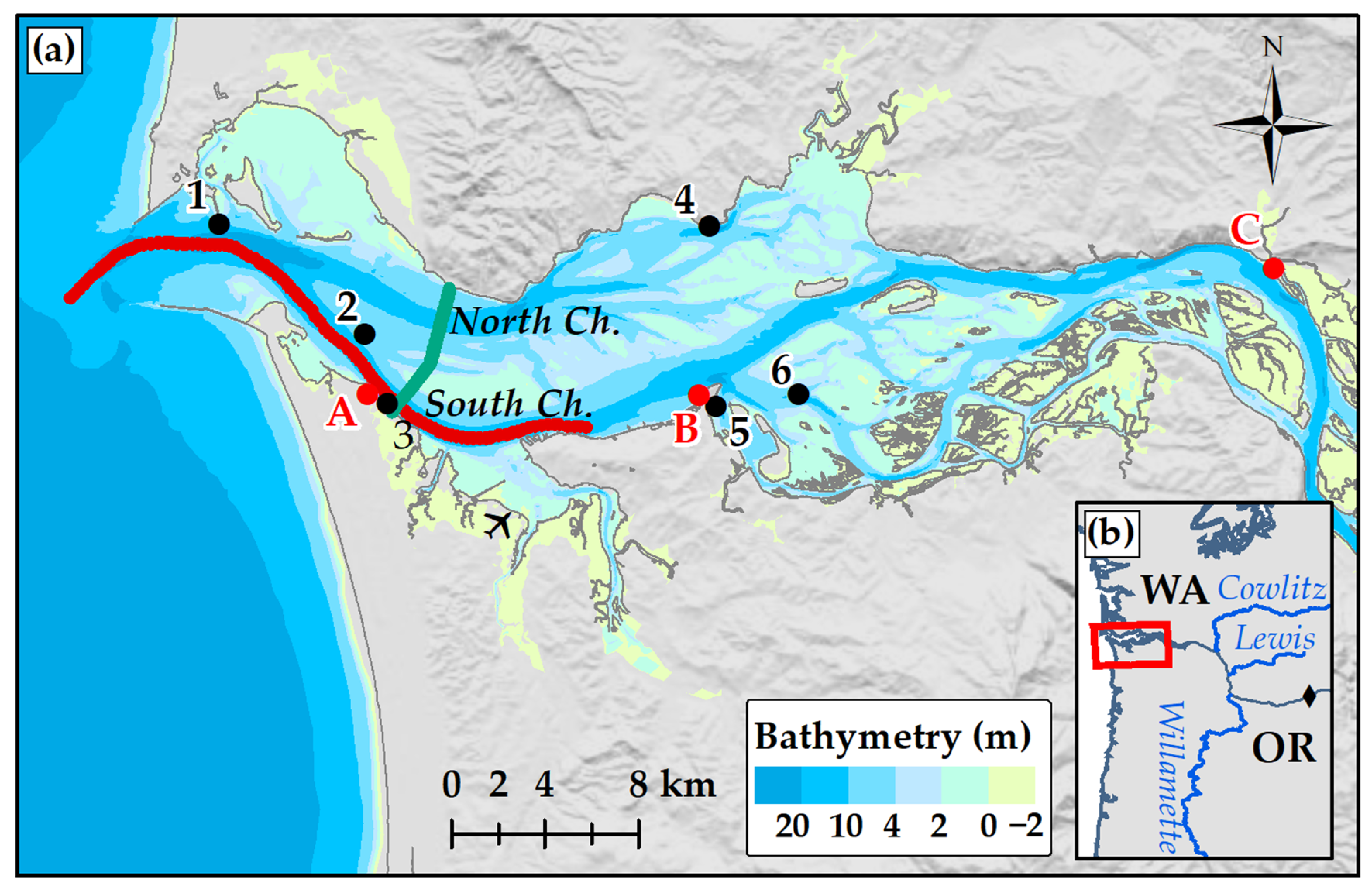
2.1. Site Description

In the Columbia River, the largest single freshwater source on the west coast of North America (Figure 1), salt intrusion defines the estuarine portion (called lower estuary) of this large river, ranging between 20 km and 50 km from the mouth. Circulation in the estuary is primarily controlled by river discharge, tides, and coastal upwelling/downwelling [20,21,27]. The tidal influence on water elevation extends upstream to 235 km from the estuary mouth [21]. The tidal pattern affecting the estuary is mixed diurnal and semidiurnal, with an amplitude ranging from 2 to 4 m near Astoria/Tongue Point [34]. The Columbia river discharge is heavily regulated and controlled by dams, the total annual mean river flow at the mouth being about 7340 m3/s [35]. Under high flows, the effect of the freshwater discharge dominates, enabling the lower estuary to remain highly stratified across all tidal conditions [21]. By contrast, at low flows the salinity structure has been described as tidally dependent [20,21].
The estuary is characterized by two narrow and deep channels (about 10 m on average), the north and south channels, with markedly different circulation characteristics [21,27]. According to Chawla et al. [27], the south channel has strong river outflow, moderate tidal currents, and a less well-developed salt-wedge, while the north channel has weaker river outflow, more tidal transport, and more salt-wedge like salinity intrusion. Thus, the two channels constitute, in effect, two rather different sub-estuaries.
Winds on the continental shelf determine coastal up- or downwelling, thus influencing the salt content and density structure of the waters entering the estuary during flood tides [36]. Ocean sources to the estuary vary from deep ocean waters during upwelling (mainly spring and summer) to more mixed surface waters during downwelling (mainly fall and winter) and relaxation. Wind-driven upwelling/downwelling summer events influence the plume of the Columbia River and its variability [27,28,29,37,38], but the estuary wind effects have been largely ignored.
WRCC [39] reports that prevailing wind direction in the estuary (Astoria airport) is from the northwest in summer and from the southwest and the west in winter, while cold easterly winds are common in winter. Strong winds from southeast to southwest usually accompany annual winter storms. Extra-tropical cyclones affect the Pacific Northwest coast, but are most common during winter, generally approaching from the southwest [40]. Winds associated with extra-tropical cyclones can exceed 50 m/s, and gusts as high as 68 m/s have been documented near the mouth of the Columbia River estuary [40].

2.2. The Model and the Simulations

We used the 3D unstructured grid, finite element SELFE model [31] that has been fully calibrated by Kärnä et al. [32] and Kärnä and Baptista [33] with atmospheric forcing from the NOAA/NCEP North American Regional Reanalysis, with a resolution of 32 km [41]. In particular, the model simulations displayed high skills in capturing the magnitude and phase of the tidal salinity intrusion for both high and low river discharge conditions, with exception during late spring/early summer high river discharge and neap tide conditions due to excessive numerical mixing.
The model domain (Figure 1), grid resolution, and bathymetry have been described in detail in Kärnä et al. [32] and Kärnä and Baptista [33]. The offshore open boundary temperature, salinity, and water elevations for this study are from the HYCOM (HYbrid Coordinate Ocean Model), a data-assimilative hybrid isopycnal-sigma-pressure (generalized) coordinate ocean model [42]. At the upstream boundary located at Bonneville Dam (Figure 1), freshwater inflows and temperature are obtained from the U.S. Geological Survey (USGS) gaging stations, while salinity is set to zero. The other minor river inputs (Willamette, Lewis, and Cowlitz; see Figure 1) are based on observational data from the USGS and U.S. Army Corps of Engineers (USACE).
The model simulations focus on the year 2014, as atmospheric forcing was available from only two databases for that period at the time of the study (see Section 2.3.2). The model was run for 3 months to warm up (from 1 October to 31 December 2013), starting with initial conditions from the forecasts and multi-year simulation databases (DB33, period 1999–2018) of the NSF Science and Technology Center for Coastal Margin Observation and Prediction (CMOP), Virtual Columbia River [43]. Model outputs at the end of 2013 were used to set the initial conditions for the year 2014.
In order to address the local wind effect on salt intrusion, we performed three simulations (see Table 1). The reference simulation (REF) was forced with the 4 km resolution Weather Research and Forecasting Model [44] atmospheric forcing (hence, WRF4, [45]). A sensitivity simulation switching off wind forcing in the estuary (NOWIND) and a simulation using the coarser resolution atmospheric forcing from the NOAA/NCEP North American Regional Reanalysis (resolution of 32 km, hence NARR32) [41] were carried out to assess the effect of wind forcing on the salinity intrusion in the estuary.

2.3. Observations

2.3.1. Monitoring Stations

An extensive interdisciplinary observation network was developed for the Columbia River estuary by the NSF Science and Technology Center for Coastal Margin Observation and Prediction (CMOP) as a part of a collaborative infrastructure for regional science and management: SATURN [43]. In addition, NOAA maintains several tidal and atmospheric stations with Columbia River relevance.
A subset of the SATURN [43] and NOAA stations (Figure 1) with 2014 observations are used for comparison with model results. In particular, the SATURN−03, SATURN−04, and CBNC3 station observations characterize the transport and mixing in the south channel, while GRAYS data are utilized for the north channel [43]. Desdemona Sands is a SATURN physical station with a central position near the mouth of the estuary, while Astoria (Tongue Point) is a NOAA−COOPS station (9439040) located on the edge of the south channel, in the middle of the lower estuary. Water elevation data are used from tide gages located at Hammond, Tongue Point, and Skamokawa stations (Figure 1).

2.3.2. Wind Forcing and River Discharge

At the time of the study, wind speed/direction observations in the estuary were available at three stations: Desdemona Sands (for the last months of 2013, the whole 2014, and partially for 2015), Astoria (for the years 2012 and 2014), and Astoria airport, from the National Weather Service (see Figure 1 for the location of the stations). The available atmospheric forcing from WRF4 started from the last months of the year 2013 up to the whole year of 2014. Thus, this study was based on the full year of 2014, the only year when both observations and WRF4/NARR32 forcing were available at the time of the study.
The wind speed and direction time series at the three available stations in the estuary and at the offshore NOAA station 46,029 were analyzed and compared to model data extracted at the nearest node of the model grid (see full description in Appendix A). Neither NARR32 nor WRF4 capture all features of the observed wind forcing (Figure A1), but WRF4 is substantially more skilled than NARR32 in the estuary. For example, NARR32 cannot reproduce the energetic easterly wind events at Desdemona station well (Figure A1 and Figure A2). Improvements in WRF4 may partially derive from a better representation of the near shore conditions, in particular during northerly winds (upwelling periods) and coastal storms.
During 2014, river discharge at Bonneville was between about 3000 m3/s and 11,000 m3/s, with lower values in winter and autumn.

2.4. Salinity Intrusion Analysis

Occasionally, in the past, salinity intrusion length data were collected for the south channel using a dedicated vessel [46,47], but measurements were labor-intensive and unfeasible with any kind of regularity. In this study, estimated data of salinity intrusion, following Monismith et al. [48], who used salinity observations in San Francisco Bay, are compared with salinity intrusion computed by the model.
Monismith et al. [48] showed there is a functional (power) relationship between the river flow (Q) and salinity intrusion (X2), given by:
X2 = aQn
where the power (negative) exponent n varies with the type of estuary [48,49]. Most investigations of salinity intrusion focus on estuaries with one primary channel, such that the whole river discharge and tidal forcing pass through that channel [48,50].
In the case of the Columbia River estuary, salinity intrusion is computed only in the south channel. The above autoregressive model applied to the long-term simulation DB33 (for the period 1999–2012, [32]) with the observed river discharge Q gives:
X2 = 580 × Q−0.366
after solving for log(X2) = n × log(Q) + C, and then: X2 = exp(C) Qn, with a = exp (C) = 580 and n = −0.366.

2.5. Mixing and Froude Number

To better understand the findings of the numerical experiments in the Columbia River estuary, the dimensionless parameters Mixing (M) and Froude number (F), as proposed by Geyer and MacCready [51] for the estuarine space, are used to assess the strength of the tide and the river discharge (in the destruction and creation of stratification in the system, respectively). The freshwater Froude number proposed by Geyer [52] is given by:
Frf = UR/(βgsoceanH )1/2
where UR is the river flow velocity, i.e., the river volume flux divided by the cross-section of the estuary, g is the gravitational acceleration, β is the haline contraction coefficient, Socean is the maximal ocean salinity, H is the depth of the estuary.
Then, the Mixing parameter:
M 2 = C D U T 2 ω N o H 2
where CD is the bottom drag coefficient, UT is the amplitude of depth-averaged tidal velocity, ω is the tidal frequency, No = (βgsocean/H)1/2, and H is the depth.
In the case of the Columbia River estuary, the two parameters of the estuarine space were computed from the cross-section at Point Adams (see the green line in Figure 1a), crossing the two channels starting from SATURN−03, as in Kärnä and Baptista [33]. Frf is directly proportional to the river discharge, scaled by the maximal speed of internal waves in the system. M, on the other hand, is proportional to tidal forcing, specifically to the bottom friction velocity u2 = CDUT2 induced by the tidal currents. N0 is the buoyancy frequency assuming linear stratification over the water column. Therefore, M2 is a ratio of tidal and mixing time scales: M≈1 implies that tidal mixing is strong enough to mix the entire water column in a half tidal cycle. The effective depth H was taken as the mean depth of the cross-section and the following constants were used, as in Kärnä and Baptista [33]: g = 9.81 ms−2, β = 7.7 × 10⁻⁴ psu−1, Socean = 34 psu.
In addition to those two parameters, we use the along-estuary component of the wind stress (τx), aligned with the main axis of the estuary, to assess the strength/direction of the wind. τx is averaged over the lower estuary area and low-pass filtered and positive/negative values represent westerly (upstream)/easterly (downstream) winds.

3. Results

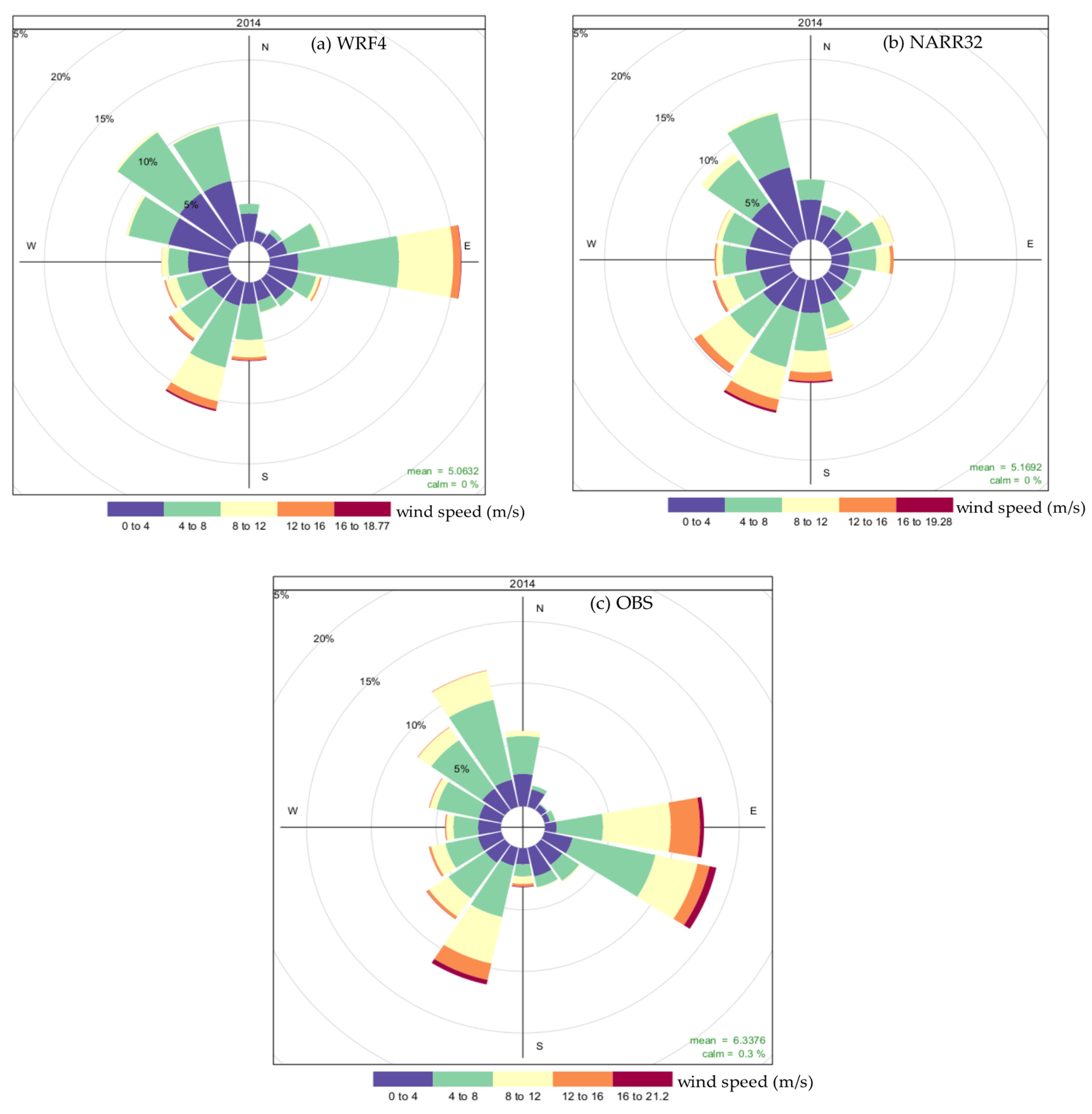
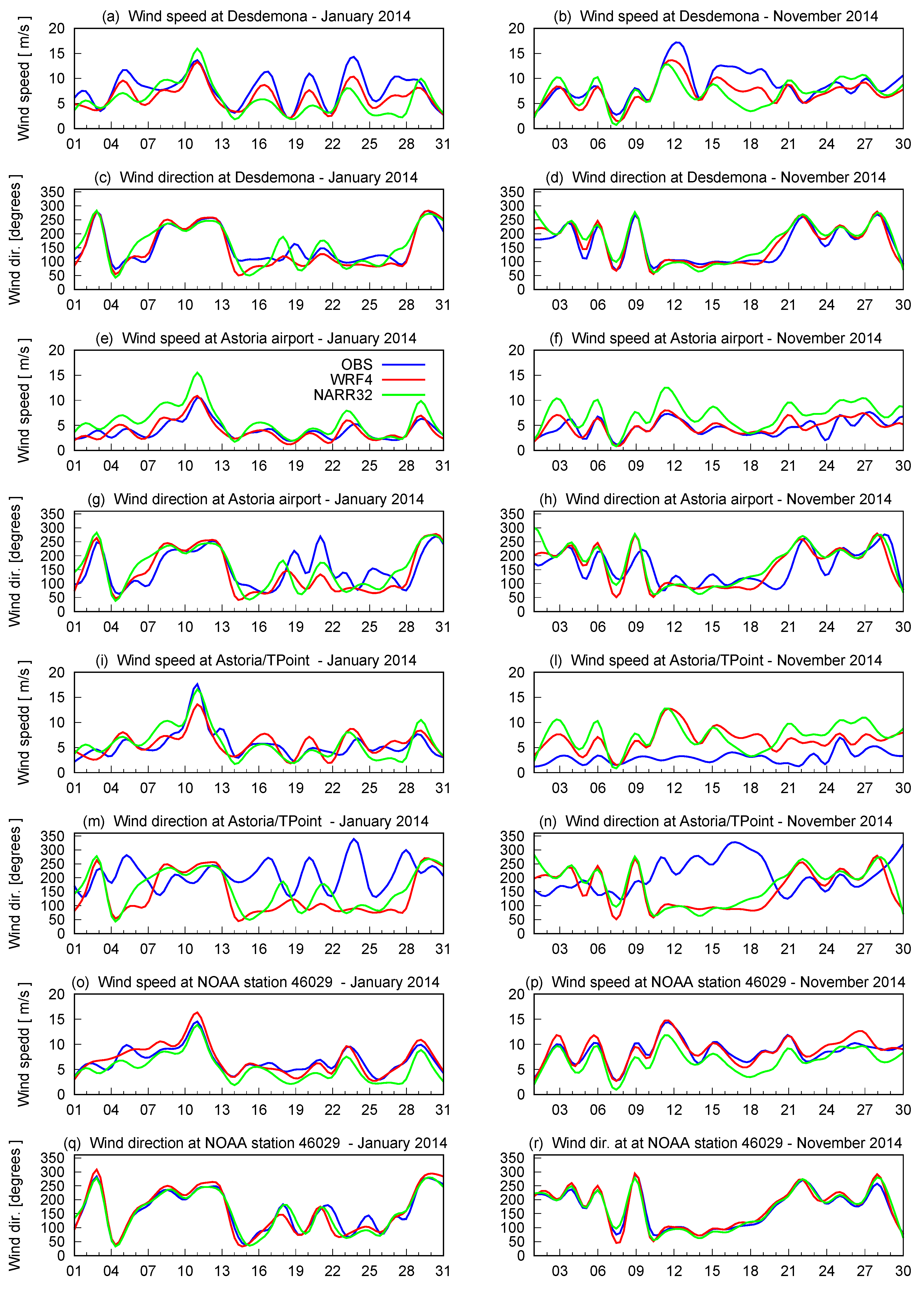
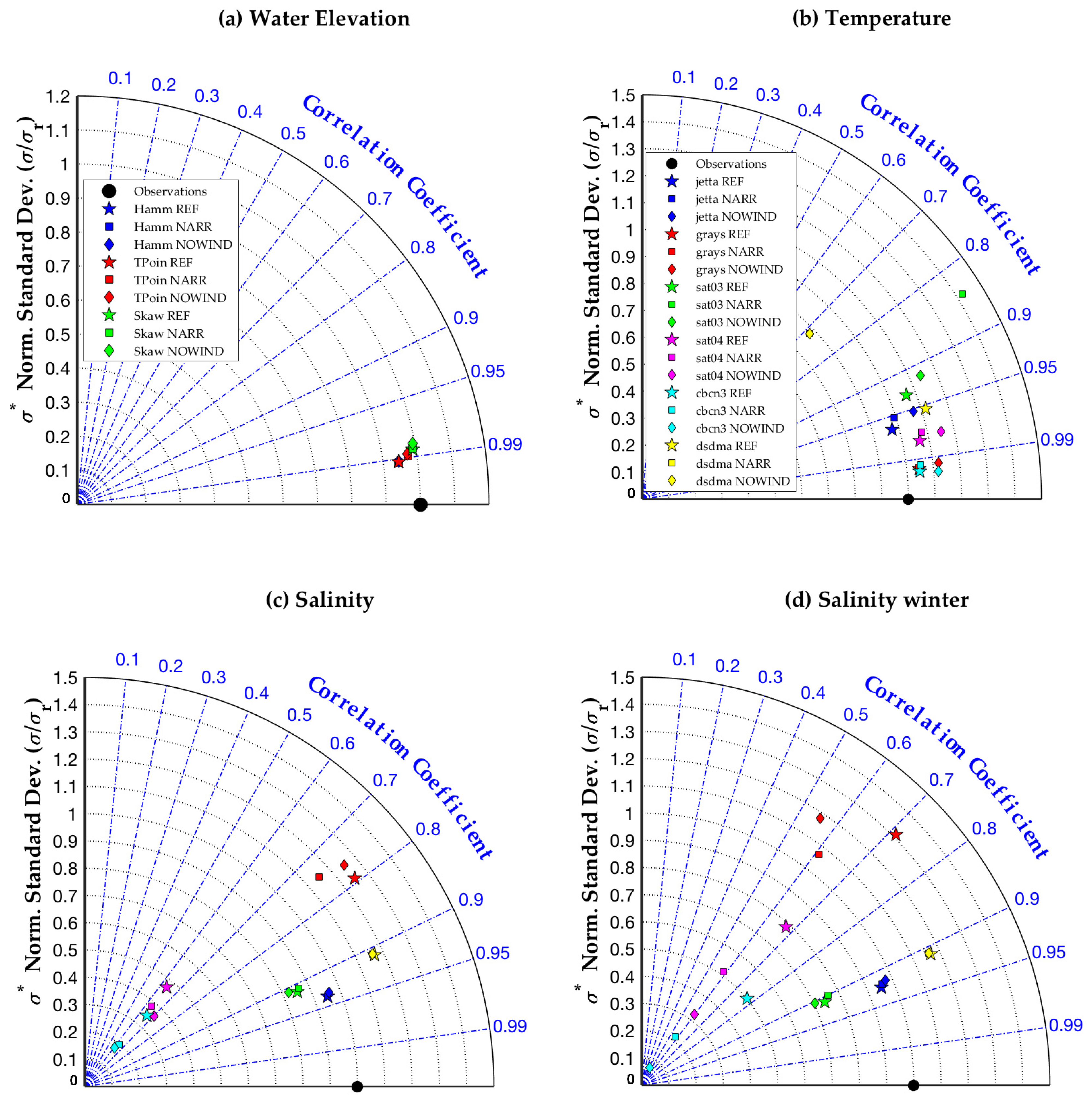
3.1. Effects of the Resolution of Atmospheric Forcing

To address the effect of wind forcing in the estuary, we first compared the modeled REF, NARR, and NOWIND water levels, near bottom temperature, and salinity with the observations. Due to the large amount of data, model results and observations were hourly averaged and then compared in the Taylor diagram plots (see Figure 2).
Both REF− and NARR−modeled water elevations at the tide gauges show very high correlations around 0.99, and a normalized standard deviation between 0.9 and 1 (Figure 2a). Similar high correlations (above 0.90), with normalized standard deviations between 0.9 and 1.2, are also shown for near-bottom temperature, except for NARR at two downstream stations, SATURN−03 and Desdemona (Figure 2b).
Full-year near-bottom salinity (Figure 2c) shows high correlation (above 0.90) and normalized standard deviation between 0.8 and 1.2 at the downstream stations (Jetta, Desdemona, and SATURN−03). Small differences are noticeable among the three runs. Results at the upstream stations—SATURN−04, cbcn3 (located in the south channel), and Grays (located in the north channel)—indicate that REF performs better than NARR. For the period January–February–November–December (Figure 2d, Salinity winter), when the river discharge is relatively low, there is a significant improvement between REF and NARR at the upstream stations, suggesting that wind forcing resolution might have more impact in fall/winter than during the rest of the year. This seasonal response is further evidenced when comparing the REF and NOWIND simulations. Indeed, significant differences in modeled salinity between REF and NOWIND are clearly noted for the upstream stations, with much more variability in winter. These differences would also indicate that local wind is important in the lower estuary, while the stations near the mouth are less influenced. Salinity intrusion might be a response to those local winds, especially during winter/fall.

3.2. Salinity Intrusion

The 2014 REF simulation (Figure 3a–e) indicates that salinity intrusion length (SIL; distance from the mouth for the 1 psu isohaline) mainly follows the seasonal pattern of the river discharge, while tidal range is approximately between 1.5 m and 3.5 m all year long. During spring/summer (fall/winter), river discharge is the highest (lowest), and, as a result, the maximum (tidal day) salinity intrusion length reaches its minimum (maximum). This strong inverse correlation between river discharge and SIL is further displayed in Table 2 for all the simulations.
In addition to responding to the seasonality of river discharge, SIL is impacted by energetic wind events during fall/winter (westerly positive, easterly negative, see Figure 3c,e) when both river discharge and tidal range are low (neap tide or beginning of spring tide). This can be further demonstrated by the two parameters M (strength of the tide) and F (strength of river discharge), as defined in Section 2.3 (Figure 3d). The peaks of the along-estuary component of the wind stress indeed correspond to low values of M and F.
The seasonal pattern of SIL from the three simulations (Figure 3e) displays, in general, similar behavior and follows the pattern of salinity intrusion X2 computed following Monismith et al. [48], indicating the impact of the river discharge on its seasonal behavior. Some discrepancies are, however, noticeable in January, February, March, November, and December, as highlighted by the yellow bands in Figure 3e, and corresponding to energetic winds events. While the three simulations give approximately the same SIL, discrepancies between them and X2 occur during March (gray band in Figure 3e) during the transition from low to high discharge. X2 calculations based on a long-time series regression might not be appropriate for event scale calculations.
In Table 2, we examine the correlation between the daily averaged river discharge and salinity intrusion from model simulations during fall/winter versus spring/summer. In fall/winter (Winter column in Table 2), the inverse correlation between river discharge and salinity intrusion is weak, suggesting that, during this period, wind plays a role in salt intrusion. The local wind effect is further evidenced by the decrease in inverse correlation between NOWIND and REF. For spring/summer (Other column in Table 2), the values are higher than for the yearly value, suggesting that river discharge is the principal forcing of the salt intrusion during that period.
The time series of differences in salinity intrusion for NOWIND−REF (blue line in Figure 4) and NARR−REF (red line in Figure 4) show some strong peaks during fall/winter. REF (higher resolution atmospheric forcing) produces farther salinity intrusion for energetic easterly wind with respect to NARR and NOWIND. During winter and autumn, NARR underestimates salinity intrusion, with an order of magnitude at times similar to the NOWIND case. During the January event with westerly wind, NARR and REF salinity intrusions are similar, but the wind effect is seen when comparing NOWIND and REF. Without local wind effects (NOWIND−REF simulations), salinity intrusions occur about 5 km farther upstream or downstream. Particularly noticeable are the events of mid-January and mid-November 2014, respectively due to energetic westerly and easterly winds, during which the maximum difference NOWIND−REF is +6.2 km in January and is −10.1 km in November.

3.3. Events of Westerly/Easterly Winds

The results presented in the previous sections show that ignoring or coarsely representing local wind forcing can introduce significant errors, and indicate some events during which episodic energetic local winds can strongly influence salinity intrusion, in particular in January and November. If we look at water levels (after removing tides) at the three tide gages during the selected wind events, it is evident that values are better resolved when local wind is included (Figure 5).
During the westerly event (January), water stack-up causes higher water levels at all of the tide gages (Figure 5a,c,e), while, during the easterly event (November), water levels are suppressed (Figure 5b,d,f). In both cases, the effect is less evident at Hammond, the station closer to the mouth, while it is more noticeable at Tongue Point, and increases more going upstream to the Skamokawa tide gauge.
To further investigate salinity intrusion during those two events, we compared the results from the REF and NOWIND simulations for tidally averaged salinity computed in the along-channel transect of the south channel (see Figure 1a, red line; Figure 6) and tidally averaged velocities over the estuary (Figure 7). During energetic westerly winds in January, a strong salinity front develops between 20 and 25 km from the mouth (Figure 6a), while during no wind conditions the salinity front expands up to 30 km (Figure 6b). During energetic easterly winds in November, bottom salt propagates farther up the estuary, more than 35 km (Figure 6c), reduced to 30 km in the absence of wind (Figure 7d). Salinity intrusion is reduced for energetic westerly wind and the opposite occurs for energetic easterly winds, while, in the absence of wind, the salinity intrusion is very similar in both events (Figure 6b–d).
For westerly winds in January (Figure 7a), surface current velocity is mainly directed up-estuary, except in the south channel, while, for easterly winds in November (Figure 7c), the currents are directed down-estuary everywhere. However, surface tidally averaged velocities in the south channel are much weaker during the westerly wind event (Figure 7a) with respect to the easterly wind period (Figure 7e), even though the wind speed is of similar magnitude. While the bottom currents are upstream in both channels, they are much weaker during the westerly event than during the easterly event. When compared to the NOWIND simulations (Figure 7b,d,f,h), we see that the westerly events lead to an intensification of the surface downstream current and a weakening of the bottom upstream currents. During easterly events, the surface downstream surface currents are intensified, as well as the upstream bottom currents.
These estuary circulation results, especially in the channels, are consistent with the classic two-layer circulation system, with inflow at the bottom and outflow at the surface. However, amplification by energetic easterly winds occurs in November (Figure 7e–g) and erosion by energetic westerly winds occurs during January (Figure 7a–d).
The plan view of the surface and bottom current structure (tidally averaged) induced within the estuary during the energetic wind events, shown in Figure 7, can be associated to the corresponding maps of bottom salinity presented in Figure 8, where results are tidally averaged and centered on the day, with isolines of salinity values equal to 1 psu (salinity intrusion). When the wind is westerly, the salinity distribution is similar in the south and north channels as the river discharge pushes more on the bottom through the longer south channel (Figure 8a). During the energetic easterly wind event, the south channel is characterized by stronger surface/bottom downstream/upstream currents, water levels in the lower estuary are suppressed, and the south channel is clearly a preferential way for salt to enter the estuary (Figure 8b). This is in line with what was reported by Chawla et al. [26], who stated that the south and north channels display different dynamics.
Finally, from the NOWIND cases, we observe that, during these two periods, the offshore wind has little impact on the difference in the salt intrusion upstream, and the preferential salinity intrusion through the south channel is strongly reduced in both January and November.

4. Discussion

The performance delivered by the model configuration with WRF4 forcing for the year 2014 shows that the model captures the main hydrographic features of the Columbia River estuary. This study focuses on the low river discharge conditions, which avoids the limitation of the SELFE model to represent the salinity structure in high flow, due to numerical mixing, as shown in Kärnä et al. [32].
The model results showed that energetic easterly and westerly winds, which align with the main axis of the estuary, have some significant effect on salinity intrusion. Ignoring local winds (NOWIND) or using coarsely (NARR) representing local winds can substantially alter salinity intrusion by more than ±5 km and differentially alter salt intrusion in the two main channels. During the year 2014, key factors for these events to occur were low river discharge (or low values of the Froude number) and simultaneous low values of the Mixing parameter, with specific conditions of magnitude of the wind (above 10–12 m/s): salinity intrusion increases/decreases for energetic easterly/westerly winds. Our finding supports the results of Jay [20], that there is barely any impact by wind when the speed is less than 10 m/s. An accurate representation of estuary winds is, therefore, necessary.
Similar to the study by Gong et al. [8] in the Pearl River estuary (China), we found that salt intrusion increases during the low−flow season of fall and winter and that local winds considerably influence it. In addition, Gong et al. [8] showed that remote and local wind effects on salt intrusion are similar, but the local wind favors an increase in salt intrusion. This finding is consistent with the case of the easterly wind in the Columbia River estuary.
Jay [20] also showed that salt intrusion in the south and north channels is very similar during low-flow conditions, but is somewhat greater in the north channel during a high-flow regime. While this is somewhat in agreement with our findings, as the response in the two channels is more similar when only remote forcing is applied, energetic easterly and westerly winds trigger different responses in the two channels during low-flow conditions, with more salinity intrusion in the south channel in the case of energetic easterly winds.
It should be noted that the present analysis addressed a specific and narrow time window of one year, with no attempt to capture the rich diversity of estuarine regimes [32] and atmospheric conditions that occur in the estuary. However, the increase in storm events observed worldwide may be one of the factors inducing enhanced saline water intrusion and impacting ecological habitats.
This study expands our understanding of the dynamics of the Columbia River estuary, but important questions remain. Further studies are warranted to fully quantify and explain the impacts of the energetic winter/fall wind events on the Columbia River estuary circulation and environment, in particular due to the interaction between local winds and remote winds. The emerging availability of high resolution forcing (also higher than WRF4) will offer opportunities to further understand these estuarine processes.
Finally, the effects of pressure gradients, the relationships among atmospheric pressure, elevation/slope, stratification, and salinity intrusion during winter storms should be further investigated in idealized simulations. In fact, the responses of the circulation in the estuary to wind conditions, not only tied to magnitude and variability thresholds, but also to duration, and/or to specific estuarine regimes, may provide important explanations as to how the combination of these factors can affect the extent and duration of salt intrusion.

5. Summary and Conclusions

While the dominance of river discharge and tides on circulation in the Columbia River is unquestionable [20,21], the recent availability of high-resolution atmospheric forcing has allowed us to explore some effects of local winds. In this study, the 3D hydrodynamic unstructured-grid finite element model SELFE was used to investigate the influence of local winds on salinity intrusion. Numerical simulations were carried out for realistic conditions of the year 2014, with 4 km and 32 km resolution atmospheric forcing. The effect of the wind was further investigated by switching it off in the estuary. Analysis of modeled salinity intrusion length showed that, in winter and fall, strong episodic wind events may exert control on this parameter. Energetic easterly winds tended to increase salinity intrusion length, while energetic westerly winds tended to do the reverse. Furthermore, the results suggested that energetic winds may differentially alter salt intrusion in the two main channels—the north and south channels—of the estuary. These findings offer motivation for future studies to better understand wind-driven interactions with tides, river discharge, and bathymetry. The relationship between wind and salinity intrusion could be important for estuary management and operations, and also for salmon habitats and biogeochemical processes.

Author Contributions

Conceptualization, I.S. and Y.H.S.; methodology, I.S., Y.H.S. and C.M.S.; software, I.S. and C.M.S.; validation, I.S. and C.M.S.; data curation, I.S. and C.M.S.; writing—original draft preparation, I.S. and Y.H.S.; writing—review and editing, I.S. and Y.H.S.; visualization, S.I and C.M.S.; supervision, Y.H.S. All authors have read and agreed to the published version of the manuscript.

Funding

This research was funded by the National Science Foundation through agreement OCE-0424602.

Data Availability Statement

Data supporting the conclusions can be accessed online: WRF4 data: https://a.atmos.washington.edu/mm5rt/ (last access on 28 November 2022), NARR32 data: https://psl.noaa.gov/data/gridded/data.narr.html (last access on 28 November 2022), SELFE model: https://bitbucket.org/cmop-dev/selfe/src/v4.0/ (last access on 28 November 2022), Observations: http://cmop.critfc.org/datamart/observation_network (last access on 28 November 2022). Please contact the correspondence author for further information.

Acknowledgments

The authors wish to thank Antonio Baptista, of Oregon Health and Science University (OHSU), for giving us access to numerical simulations conducted by Paul Turner under his scientific supervision. Special thanks go to Paul Turner, who carried out the simulations on Texas Advanced Computing Center (TACC) Stampede cluster, at the University of Texas, Austin. We also acknowledge all the colleagues of the Baptista group at CMOP/OHSU at the time the research was carried out, in particular Tuomas Kärnä and Jesse Lopez. At that time, Isabella Scroccaro and Charles Seaton were working in the Baptista group, as post-doctoral fellow and researcher, respectively. The authors wish to thank Georg Umgiesser of ISMAR−CNR in Venice for the useful discussion.

Conflicts of Interest

The authors declare no conflict of interest. The funders had no role in the design of the study; in the collection, analyses, or interpretation of data; in the writing of the manuscript, or in the decision to publish the results.

Appendix A

To verify how effective the applied wind forcing is at modeling actual conditions, the time series of observed wind speed and direction at the three available stations in the estuary and at offshore NOAA station 46029 are compared to modeled wind speed and direction from both WRF4 and NARR32 for the whole year and during the two events of January and November 2014 (Figure A1 and Figure A2).
The wind forcing from WRF4 can quite correctly represent the wind speed in the estuary at Desdemona and Astoria airport, while NARR32 tends to underestimate the wind speed at Desdemona and overestimate it at Astoria airport (Figure A2a,b,e,f).
Westerly winds during the event in January and easterly winds during the event in November are fairly performed by both WRF4 and NARR32 (Figure A2c,d,g,h), but WRF4 is substantially more skilled, especially during easterly winds. Both WRF4 and NARR32 can represent the westerly wind event at Astoria/Tongue Point in January, but the observations do not show the modeled easterly wind event in November (Figure A2m,n). Most likely, this is due to the geographic feature of this station, being fairly sheltered, and therefore, not representative of the wind in the estuary.
Figure A1. Wind rose plots for the year 2014 at Desdemona Sands station, with frequency of counts by wind direction. (a) Wind speed from WRF4 model and (b) wind speed from NARR32 model; (c) wind speed from observations. The direction indicates where wind is blowing from.
Water 15 00326 g0a1
Figure A2. Time series of wind speed and direction at the three available stations in the estuary and at offshore NOAA station 46029, from observations, WRF4 and NARR32, in January and November 2014. (ad) Desdemona; (eh) Astoria airport; (in) Astoria/Tongue Point; (or) NOAA station 46029. The red and green lines refer to WRF4 and NARR32, respectively. The blue line refers to the observations.
Water 15 00326 g0a2
Finally, wind direction at NOAA station 46029 (Figure A2o–r) also shows that, on the shelf close to the river mouth, winds are westerly in January and easterly in November, but wind speed is better represented by WRF4.
The distribution of the WRF4 wind speed fields during the two events of January and November 2014 show that winds are energetic and quite spatially uniform in the central part of the estuary and in the shelf, ranging from 12 m/s up to 16 m/s, with peak values of wind speed in the north channel during the event of November (Figure A3). Therefore, the main wind directions align with the axis of the estuary, with westerly winds blowing up-estuary and easterly winds down-estuary for both remote and local winds.
Figure A3. Maps of the modeled wind speed spatial variability over the Columbia River estuary. (a) Events of January and (b) November 2014 from the reference simulation with WRF4. During the two events, the wind is energetic in the central part of the lower estuary, with a peak in the north channel for the case of November.
Water 15 00326 g0a3

References

  1. North, E.W.; Chao, S.Y.; Sanford, L.P.; Hood, R.R. The influence of wind and river pulses on an estuarine turbidity maximum: Numerical studies and field observations in Chesapeake Bay. Estuaries 2004, 27, 132–146. [Google Scholar] [CrossRef]
  2. Cloern, J.E.; Jassby, A.D.; Schraga, T.S.; Nejad, E.; Martin, C. Ecosystem variability along the estuarine salinity gradient: Examples from long-term study of San Francisco Bay. Limnol. Oceanogr. 2017, 62, S272–S291. [Google Scholar] [CrossRef] [Green Version]
  3. Gillanders, B.M.; Kingsford, M.J. Impact of changes in flow of freshwater on estuarine and open coastal habitats and the associated organisms. In Oceanography and Marine Biology: An Annual Review; Gibson, R.N., Barnes, M., Atkinson, R.J.A., Eds.; Taylor & Francis: Abingdon, UK, 2002; Volume 40, pp. 233–309. [Google Scholar]
  4. Tian, R. Factors controlling saltwater intrusion across multi-time scales in estuaries, Chester River, Chesapeake Bay. Estuarine Coast. Shelf Sci. 2019, 223, 61–73. [Google Scholar] [CrossRef]
  5. Dijkstra, Y.M.; Schuttelaars, H.M. A Unifying Approach to Subtidal Salt Intrusion Modeling in Tidal Estuaries. J. Phys. Oceanogr. 2021, 51, 147–167. [Google Scholar] [CrossRef]
  6. Bellafiore, D.; Ferrarin, C.; Maicu, F.; Manfè, G.; Lorenzetti, G.; Umgiesser, G.; Zaggia, L.; Levinson, A.V. Saltwater Intrusion in a Mediterranean Delta Under a Changing Climate. J. Geophys. Res. Oceans 2021, 126, 1–23. [Google Scholar] [CrossRef]
  7. Reyes-Merlo, M.Á.; Díez-Minguito, M.; Ortega-Sánchez, M.; Baquerizo, A.; Losada, M.Á. On the relative influence of climate forcing agents on the saline intrusion in a well-mixed estuary: Medium-term Monte Carlo predictions. J. Coast. Res. 2013, 165, 1200–1205. [Google Scholar] [CrossRef]
  8. Gong, W.; Lin, Z.; Chen, Y.; Chen, Z.; Zhang, H. Effect of winds and waves on salt intrusion in the Pearl River estuary. Ocean Sci. 2018, 14, 139–159. [Google Scholar] [CrossRef] [Green Version]
  9. Zhou, W.; Wang, D.; Luo, L. Investigation of saltwater intrusion and salinity stratification in winter of 2007/2008 in the Zhujiang River Estuary in China. Acta Oceanol. Sin. 2012, 31, 31–46. [Google Scholar] [CrossRef]
  10. Zhang, E.; Gao, S.; Savenije, H.H.; Si, C.; Cao, S. Saline water intrusion in relation to strong winds during winter cold outbreaks: North Branch of the Yangtze Estuary. J. Hydrol. 2019, 574, 1099–1109. [Google Scholar] [CrossRef]
  11. Jongbloed, H.; Schuttelaars, H.M.; Dijkstra, Y.M.; Donkers, P.B.; Hoitink, A.J.F. Influence of Wind on Subtidal Salt Intrusion and Stratification in Well-Mixed and Partially Stratified Estuaries. J. Phys. Oceanogr. 2022, 52, 3139–3158. [Google Scholar] [CrossRef]
  12. Reyes-Hernández, C.; Valle-Levinson, A. Wind Modifications to Density-Driven Flows in Semienclosed, Rotating Basins. J. Phys. Oceanogr. 2010, 40, 1473–1487. [Google Scholar] [CrossRef]
  13. Jia, P.; Li, M. Dynamics of wind-driven circulation in a shallow lagoon with strong horizontal density gradient. J. Geophys. Res. 2012, 117, C05013. [Google Scholar] [CrossRef]
  14. Kim, C.-K.; Park, K. A modeling study of water and salt exchange for a micro-tidal, stratified northern Gulf of Mexico estuary. J. Mar. Syst. 2012, 96-97, 103–115. [Google Scholar] [CrossRef]
  15. Li, Y.; Li, M. Wind-driven lateral circulation in a stratified estuary and its effects on the along-channel flow. J. Geophys. Res. 2012, 117, C09005. [Google Scholar] [CrossRef] [Green Version]
  16. Li, Y.; Li, M. Effects of winds on stratification and circulation in a partially mixed estuary. J. Geophys. Res. 2011, 116, C12012. [Google Scholar] [CrossRef]
  17. Geyer, W. Influence of Wind on Dynamics and Flushing of Shallow Estuaries. Estuar. Coast. Shelf Sci. 1997, 44, 713–722. [Google Scholar] [CrossRef]
  18. Wang, D.-P. Wind-Driven Circulation in the Chesapeake Bay, Winter, 1975. J. Phys. Oceanogr. 1979, 9, 564–572. [Google Scholar] [CrossRef]
  19. Scully, M.E.; Friedrichs, C.; Brubaker, J. Control of estuarine stratification and mixing by wind-induced straining of the estuarine density field. Estuaries 2005, 28, 321–326. [Google Scholar] [CrossRef]
  20. Jay, D.A. Circulatory Processes in the Columbia River Estuary; Columbia River Estuary Data Development Program: Astoria, OR, USA, 1984; 169p. [Google Scholar]
  21. Jay, D.A.; Smith, J.D. Circulation, density structure and neap-spring transitions in the Columbia River Estuary. Prog. Oceanogr. 1990, 25, 81–112. [Google Scholar] [CrossRef]
  22. Baptista, A.M.; Zhang, Y.L.; Chawla, A.; Zulauf, M.; Seaton, C.; Myers, E.P., III; Kindle, J.; Wilkin, M.; Burla, M.; Turner, P.J. A cross-scale model for 3D baroclinic circulation in estuary-plume-shelf systems: II. Application to the Columbia River. Cont. Shelf Res. 2005, 25, 935–972. [Google Scholar] [CrossRef]
  23. Liu, Y.; MacCready, P.; Hickey, B.M.; Dever, E.P.; Kosro, P.M.; Banas, N.S. Evaluation of a coastal ocean circulation model for the Columbia River plume in summer 2004. J. Geophys. Res. Oceans 2009, 114, 1–23. [Google Scholar] [CrossRef] [Green Version]
  24. Elias, E.P.L.; Gelfenbaum, G.; Van der Westhuysen, A.J. Validation of a coupled wave-flow model in a high-energy setting: The mouth of the Columbia River. J. Geophys. Res. Oceans 2012, 117, C09011. [Google Scholar] [CrossRef]
  25. Jay, D.A.; Leffler, K.; Diefenderfer, H.L.; Borde, A.B. Tidal-Fluvial and Estuarine Processes in the Lower Columbia River: I. Along-Channel Water Level Variations, Pacific Ocean to Bonneville Dam. Estuaries Coasts 2014, 38, 415–433. [Google Scholar] [CrossRef]
  26. Helaire, L.T.; Talke, S.A.; Jay, D.A.; Mahedy, D. Historical Changes in Lower Columbia River and Estuary Floods: A Numerical Study. J. Geophys. Res. Oceans 2019, 124, 7926–7946. [Google Scholar] [CrossRef]
  27. Chawla, A.; Jay, D.A.; Baptista, A.; Wilkin, M.; Seaton, C. Seasonal Variability and Estuary–Shelf Interactions in Circulation Dynamics of a River-dominated Estuary. Estuaries Coasts 2008, 31, 269–288. [Google Scholar] [CrossRef] [Green Version]
  28. MacCready, P.; Banas, N.; Hickey, B.M.; Dever, E.P.; Liu, Y. A model study of tide- and wind-induced mixing in the Columbia River Estuary and plume. Cont. Shelf Res. 2009, 29, 278–291. [Google Scholar] [CrossRef]
  29. Burla, M.; Baptista, A.M.; Zhang, Y.; Frolov, S. Seasonal and interannual variability of the Columbia River plume: A perspective enabled by multiyear simulation databases. J. Geophys. Res. Oceans 2010, 115, C00B16. [Google Scholar] [CrossRef]
  30. Giddings, S.N.; MacCready, P. Reverse Estuarine Circulation Due to Local and Remote Wind Forcing, Enhanced by the Presence of Along-Coast Estuaries. J. Geophys. Res. Oceans 2017, 122, 10184–10205. [Google Scholar] [CrossRef] [Green Version]
  31. Zhang, Y.; Baptista, A.M. SELFE: A semi-implicit Eulerian–Lagrangian finite-element model for cross-scale ocean circulation. Ocean Model. 2008, 21, 71–96. [Google Scholar] [CrossRef]
  32. Kärnä, T.; Baptista, A.M.; Lopez, J.E.; Turner, P.J.; McNeil, C.; Sanford, T.B. Numerical modeling of circulation in high-energy estuaries: A Columbia River estuary benchmark. Ocean Model. 2015, 88, 54–71. [Google Scholar] [CrossRef]
  33. Kärnä, T.; Baptista, A. Evaluation of a long-term hindcast simulation for the Columbia River estuary. Ocean Model. 2016, 99, 1–14. [Google Scholar] [CrossRef] [Green Version]
  34. Kukulka, T.; Jay, D.A. Impacts of Columbia River discharge on salmonid habitat: 1. A nonstationary fluvial tide model. J. Geophys. Res. Oceans 2003, 108, 3293. [Google Scholar] [CrossRef] [Green Version]
  35. Naik, P.K.; Jay, D.A. Distinguishing human and climate influences on the Columbia River: Changes in mean flow and sediment transport. J. Hydrol. 2011, 404, 259–277. [Google Scholar] [CrossRef]
  36. Jay, D.A.; Smith, J.D. Residual circulation in shallow estuaries: 1. Highly stratified, narrow estuaries. J. Geophys. Res. 1990, 95, 711–731. [Google Scholar] [CrossRef] [Green Version]
  37. Hickey, B.M.; Banas, N. Oceanography of the U.S. Pacific Northwest Coastal Ocean and estuaries with application to coastal ecology. Estuaries 2003, 26, 1010–1031. [Google Scholar] [CrossRef]
  38. Hickey, B.; Geier, S.; Kachel, N.; MacFadyen, A. A bi-directional river plume: The Columbia in summer. Cont. Shelf Res. 2005, 25, 1631–1656. [Google Scholar] [CrossRef]
  39. WRCC (Western Regional Climate Center) Period of Record Monthly Climate Summary, Astoria, Oregon (350324). 2009. Available online: http://www.wrcc.dri.edu/cgi-bin/cliMAIN.pl?or0324 (accessed on 28 November 2022).
  40. Mass, C.; Dotson, B. Major Extratropical Cyclones of the Northwest United States: Historical Review, Climatology, and Synoptic Environment. Mon. Weather. Rev. 2010, 138, 2499–2527. [Google Scholar] [CrossRef]
  41. Mesinger, F.; Di Mego, G.; Kalnay, E.; Mitchell, K.; Shafran, P.C.; Ebisuzaki, W.; Jović, D.; Woollen, J.; Rogers, E.; Berbery, E.H.; et al. North American Regional Reanalysis. Bull. Am. Meteorol. Soc. 2006, 87, 343–360. [Google Scholar] [CrossRef] [Green Version]
  42. Bleck, R. An oceanic general circulation model framed in hybrid isopycnic-Cartesian coordinates. Ocean Model. 2002, 4, 55–88. [Google Scholar] [CrossRef]
  43. Baptista, A.M.; Seaton, C.; Wilkin, M.P.; Riseman, S.F.; Needoba, J.A.; Maier, D.; Turner, P.J.; Kärnä, T.; Lopez, J.E.; Herfort, L.; et al. Infrastructure for collaborative science and societal applications in the Columbia River estuary. Front. Earth Sci. 2015, 9, 659–682. [Google Scholar] [CrossRef]
  44. Michalakes, J.; Dudhia, J.; Gill, D.; Henderson, T.; Klemp, J.; Skamarock, W.; Wang, W. The Weather Research and Forecast Model: Software Architecture and Performance. In Proceedings of the Eleventh ECMWF Workshop on the Use of High Performance Computing in Meteorology, Reading, UK, 25–29 October 2004; Zwieflhofer, W., Mozdzynski, G., Eds.; World Scientific: Singapore, 2005; pp. 156–168. [Google Scholar]
  45. Brewer, M.C.; Mass, C.F. Simulation of Summer Diurnal Circulations over the Northwest United States. Weather. Forecast. 2014, 29, 1208–1228. [Google Scholar] [CrossRef]
  46. Baptista, A.M.; Wilkin, M.; Pearson, P.; Turner, P.; McCandlish, C.; Barrett, P. Coastal and estuarine forecast systems—A multi-purpose infrastructure for the Columbia River. Earth Syst. Monit. 1999, 9, 1–2+4. [Google Scholar]
  47. Baptista, A.M. CORIE: The first decade of a coastal-margin collaborative observatory. In Proceedings of the Oceans’06 MTS/IEEE, Boston, MA, USA, 18–21 September 2006. [Google Scholar]
  48. Monismith, S.G.; Kimmerer, W.; Burau, J.R.; Stacey, M.T. Structure and Flow-Induced Variability of the Subtidal Salinity Field in Northern San Francisco Bay. J. Phys. Oceanogr. 2002, 32, 3003–3019. [Google Scholar] [CrossRef]
  49. Bowen, M.M. Salt transport and the time-dependent salt balance of a partially stratified estuary. J. Geophys. Res. Atmos. 2003, 108, C5. [Google Scholar] [CrossRef]
  50. Ralston, D.K.; Geyer, W.R.; Lerczak, J.A. Subtidal Salinity and Velocity in the Hudson River Estuary: Observations and Modeling. J. Phys. Oceanogr. 2008, 38, 753–770. [Google Scholar] [CrossRef] [Green Version]
  51. Geyer, W.R.; MacCready, P. The Estuarine Circulation. Annu. Rev. Fluid Mech. 2014, 46, 175–197. [Google Scholar] [CrossRef]
  52. Geyer, W.R. Estuarine salinity structure and circulation. In Contemporary Issues in Estuarine Physics; Valle-Levinson, A., Ed.; Cambridge University Press: Cambridge, UK, 2010; Chapter 2; pp. 12–26. [Google Scholar]
Figure 1. Map with (a) bathymetry and (b) location of the Columbia River estuary between Oregon (OR) and Washington States (WA). The black dots in (a) indicate the locations of the observational stations used in the study. 1: Jetta; 2: Desdemona sands (DSDMA); 3: SATURN−03, 4: Grays; 5: SATURN−04; 6: CBCN3. The red dots represent the tide gauges. A: Hammond; B: Astoria/Tongue Point (TPOIN); C: Skamokawa. The airplane symbol indicates Astoria airport. The red line represents the along-channel transect of the South channel, while the green line represents the cross-channel transect, starting from SATURN−03 station, referred to as transect of Point Adams. Offshore NOAA station 46,029 is about 40 km west from the mouth. The black diamond in (b) indicates Bonneville Dam, the upstream limit of the domain, while Cowlitz, Lewis, and Willamette indicate the minor river inputs (in blue).
Water 15 00326 g001
Figure 2. Taylor diagram plots of the three simulations REF, NARR, and NOWIND. (a) Water elevation, full year 2014. Results for the Hammond station (in blue) are almost overlapping and are covered by the red star symbol of Tongue Point station (TPoin); (b) near bottom temperature, full year 2014; (c) near bottom salinity, the full year 2014; (d) near bottom salinity for the winter period only. Winter represents the months of January, February, November, and December. The legend for (c) Salinity and (d) Salinity winter is the same as in (b) Temperature.
Water 15 00326 g002
Figure 3. Time series of the year 2014 for the reference simulation: (a) river discharge at Bonneville; (b) tidal range at SATURN−03; (c) along-estuary wind stress τx from the reference simulation (with WRF4); (d) Mixing and Froude number at cross-section of Point Adams; (e) maximum (tidal day) salinity intrusion length from model results (REF, NARR, and NOWIND) vs. X2 computed from river discharge (X2Q), by using the method described by Monismith et al. [48]. The yellow vertical bands indicate the peaks of along-estuary wind stress, while the gray area highlights the period during which the river discharge and, consequently, the Froud number are increasing up to their maximum.
Water 15 00326 g003
Figure 4. Time series of the difference in salinity intrusion length between the NOWIND (NOW−REF), NARR simulation (NARR−REF), and the REF model simulation. The green horizontal band represents the range between −2 km and +2 km, while the yellow vertical bands and the grey area are as in Figure 3.
Water 15 00326 g004
Figure 5. Time series of water level (after removing tides) at the three available tide gauges. Data at Hammond were not available in November 2014. The red and blue lines refer to the REF and NOWIND simulations, respectively. The black line refers to the observations.
Water 15 00326 g005
Figure 6. Tidally averaged salinity structure in the along-channel transect of the south channel. (a,b) event of January and (c,d) event of November 2014. Results from the reference simulation (a,c) are compared with results from the NOWIND run (b,d). In order to better visualize the difference in salinity intrusion, the range for salinity was intentionally set to 0–10 psu.
Water 15 00326 g006
Figure 7. Tidally averaged velocity over the estuary during the events of January and November 2014. (a) Surface for REF and (b) NOWIND in January. (c) Bottom for REF and (d) NOWIND in January. (e) Surface for REF and (f) NOWIND in November. (g) Bottom for REF and (h) NOWIND in November.
Water 15 00326 g007
Figure 8. Maps of bottom REF salinity (psu), tidally averaged and centered on the day, with isolines of salinity values equal to 1 psu (red line). (a) Event of January and (b) event of November 2014. The green line indicates the 1 psu salinity for the NOWIND simulation.
Water 15 00326 g008
Table 1. Summary of the numerical simulations of 2014 used in this study.
SimulationDescription
REFHigh resolution atm. forcing from WRF4 (4 km) in both shelf and estuary (reference)
NOWINDHigh resolution atm. forcing from WRF4 (4 km) in the shelf and no wind in the estuary
NARRLow-medium atm. forcing from NARR32 (32 km) in both shelf and estuary
Table 2. Correlations between river discharge and salinity intrusion length (SIL), computed for different periods of the year 2014. Winter represents the months of January–February–November–December, while Other is the rest of the year.
SIL vs. DischargeFull YearWinterOther
REF−0.8030−0.2382−0.9107
NOWIND−0.8326−0.3217−0.9092
NARR−0.8117−0.2636−0.9052
Disclaimer/Publisher’s Note: The statements, opinions and data contained in all publications are solely those of the individual author(s) and contributor(s) and not of MDPI and/or the editor(s). MDPI and/or the editor(s) disclaim responsibility for any injury to people or property resulting from any ideas, methods, instructions or products referred to in the content.

