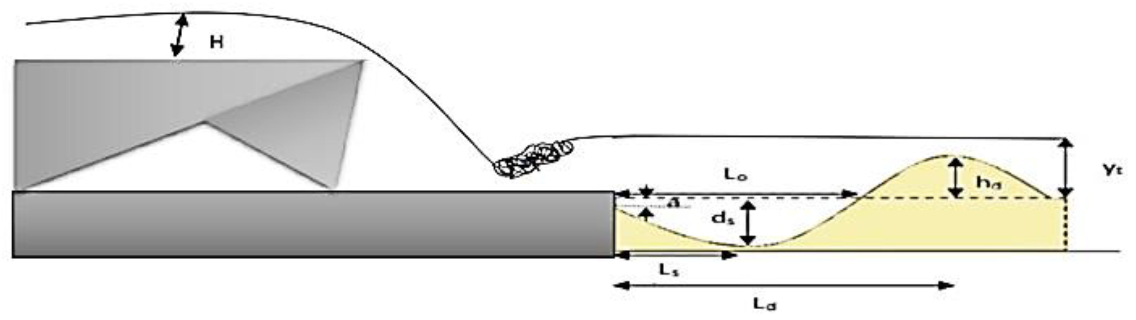
Figure 1.
Schematic view of scour hole and its characteristic parameters.
Figure 1.
Schematic view of scour hole and its characteristic parameters.
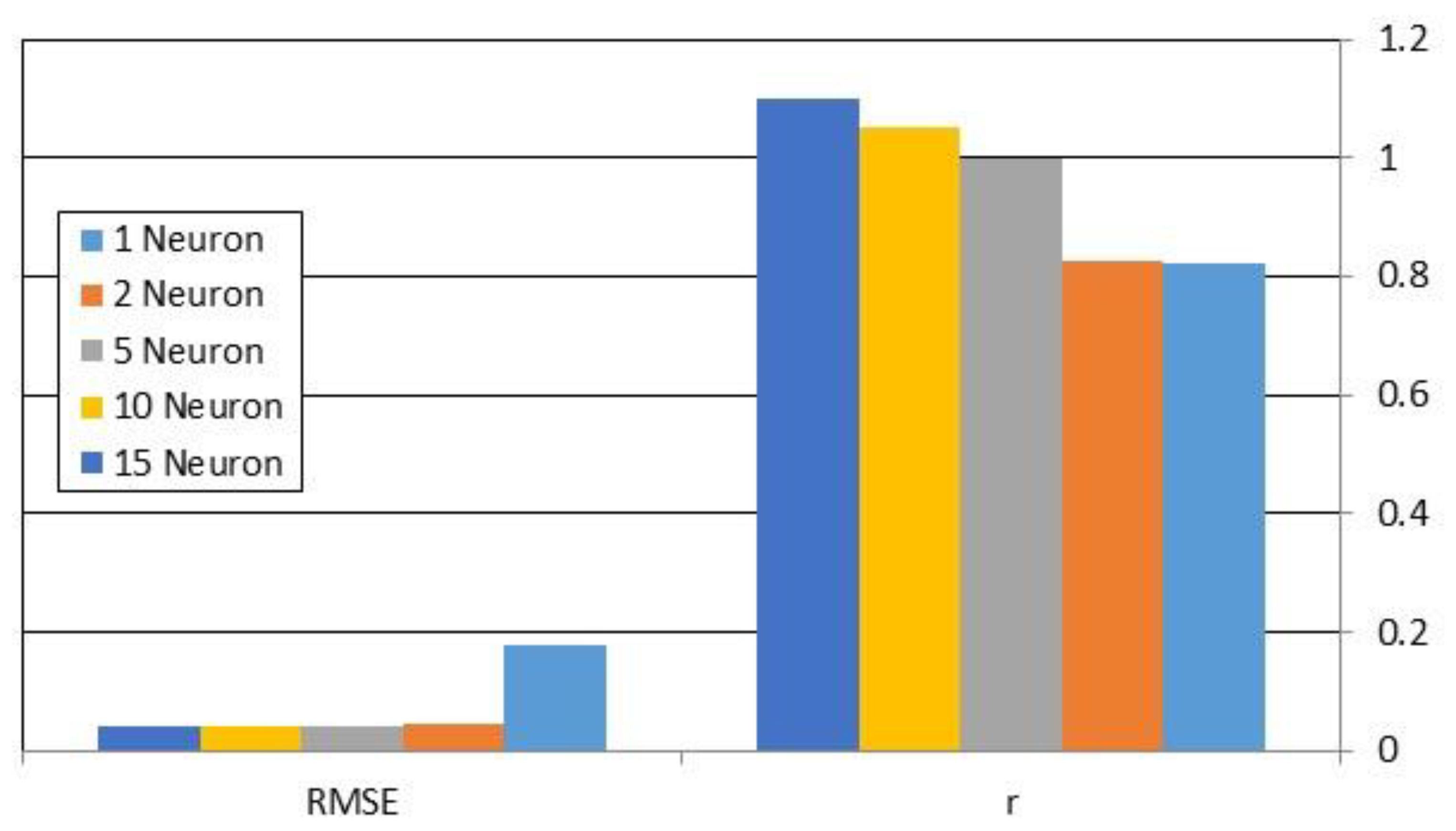
Figure 2.
Verification indicators for networks with different numbers of neurons. Note. RMSE: Root means square error.
Figure 2.
Verification indicators for networks with different numbers of neurons. Note. RMSE: Root means square error.
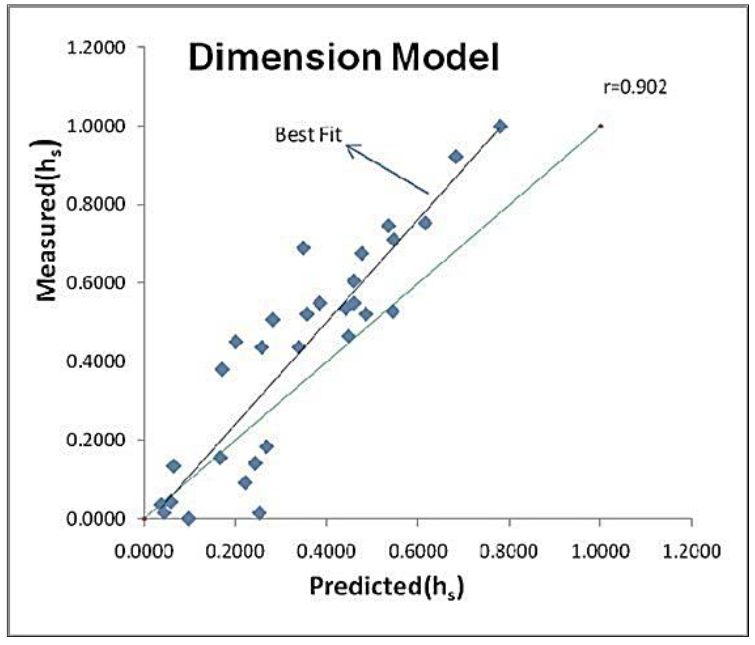
Figure 3.
Performance of the dimensional model when estimating the depth of the scour hole in the network with ten neurons in the hidden layer.
Figure 3.
Performance of the dimensional model when estimating the depth of the scour hole in the network with ten neurons in the hidden layer.
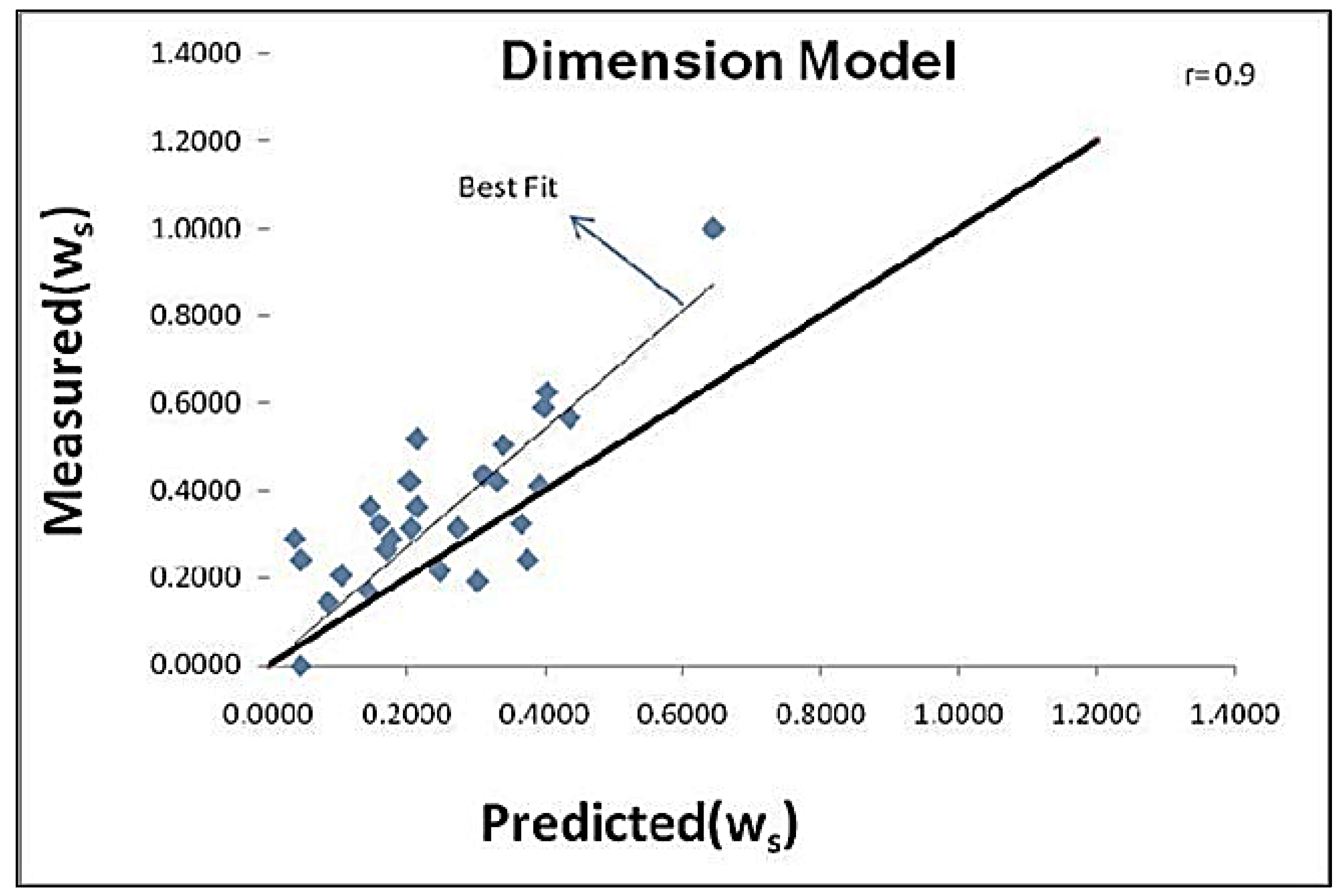
Figure 4.
Performance of the dimensional model when estimating the width of the scour hole in the network with ten neurons in the hidden layer.
Figure 4.
Performance of the dimensional model when estimating the width of the scour hole in the network with ten neurons in the hidden layer.
Figure 5.
Performance of the dimensionless model in estimating the height of the scour hole in the network with ten neurons in the hidden layer.
Figure 5.
Performance of the dimensionless model in estimating the height of the scour hole in the network with ten neurons in the hidden layer.
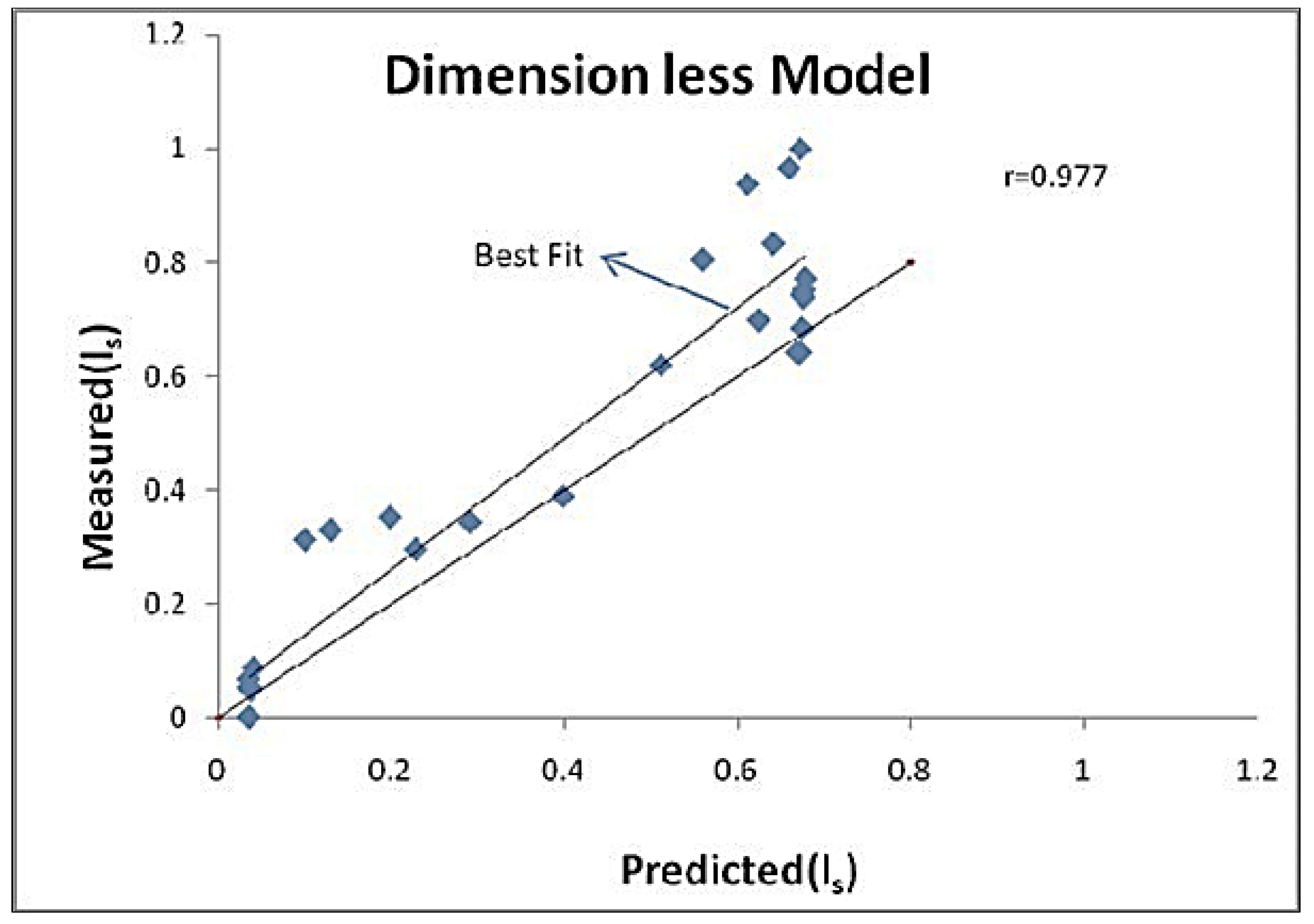
Figure 6.
Performance of the dimensionless model when estimating the length of the scour hole in the network with ten neurons in the hidden layer.
Figure 6.
Performance of the dimensionless model when estimating the length of the scour hole in the network with ten neurons in the hidden layer.
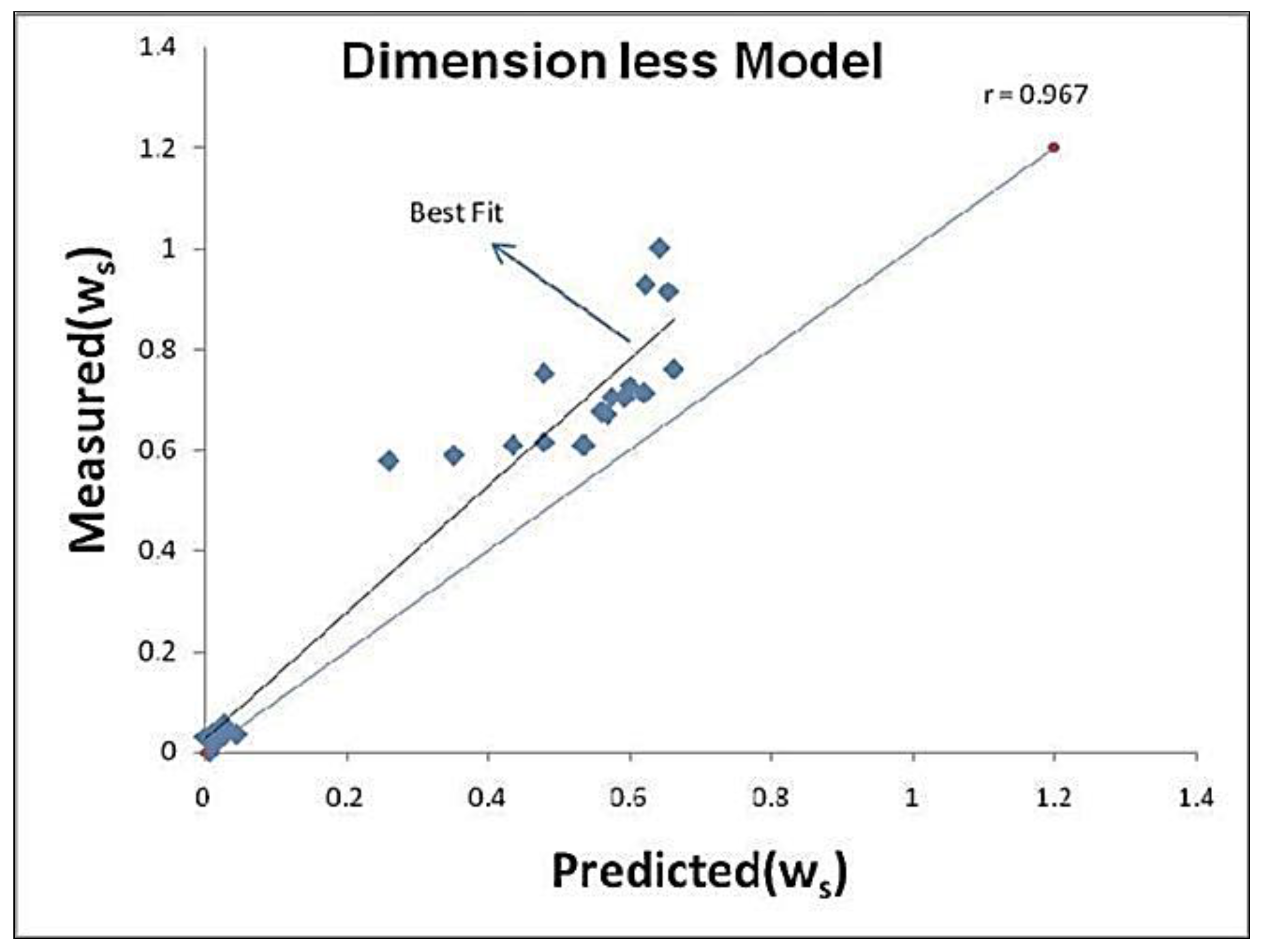
Figure 7.
Performance of the dimensionless model when estimating the width of the scour hole in the network with ten neurons in the hidden layer.
Figure 7.
Performance of the dimensionless model when estimating the width of the scour hole in the network with ten neurons in the hidden layer.
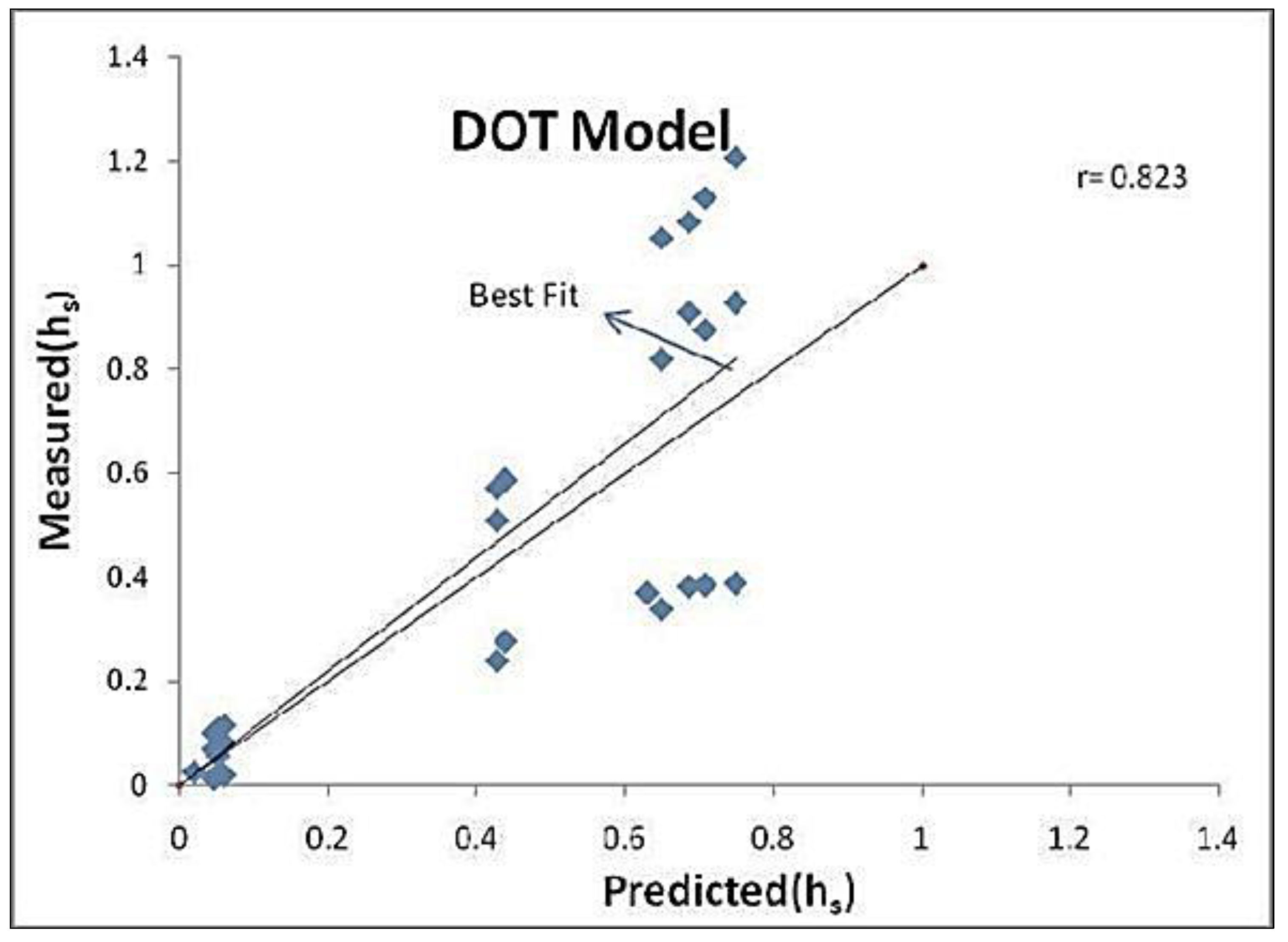
Figure 8.
Performance of the DOT model when estimating the height of the scour hole in the network with one neuron in the hidden layer.
Figure 8.
Performance of the DOT model when estimating the height of the scour hole in the network with one neuron in the hidden layer.
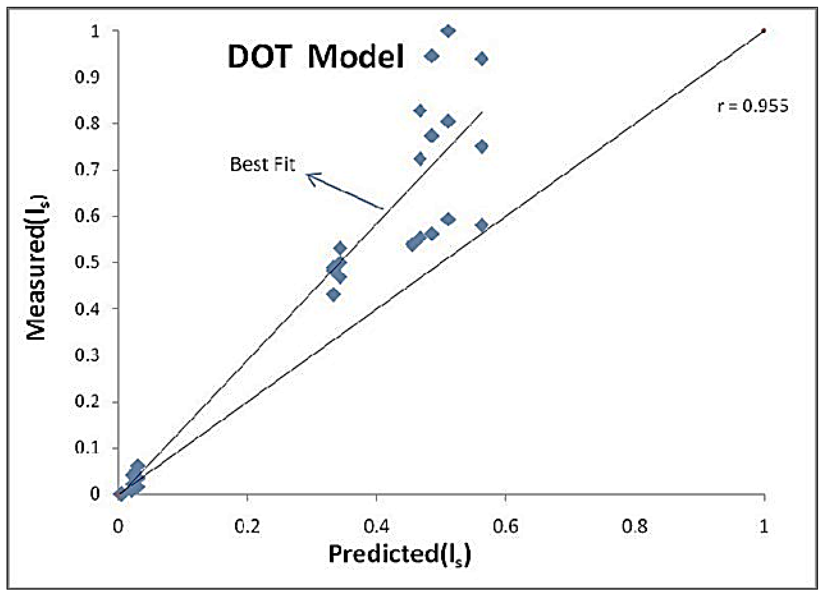
Figure 9.
Performance of the DOT model when estimating the length of the scour hole in the network with one neuron in the hidden layer.
Figure 9.
Performance of the DOT model when estimating the length of the scour hole in the network with one neuron in the hidden layer.
Figure 10.
Performance of the DOT model when estimating the width of the scour hole in the network with one neuron in the hidden layer.
Figure 10.
Performance of the DOT model when estimating the width of the scour hole in the network with one neuron in the hidden layer.
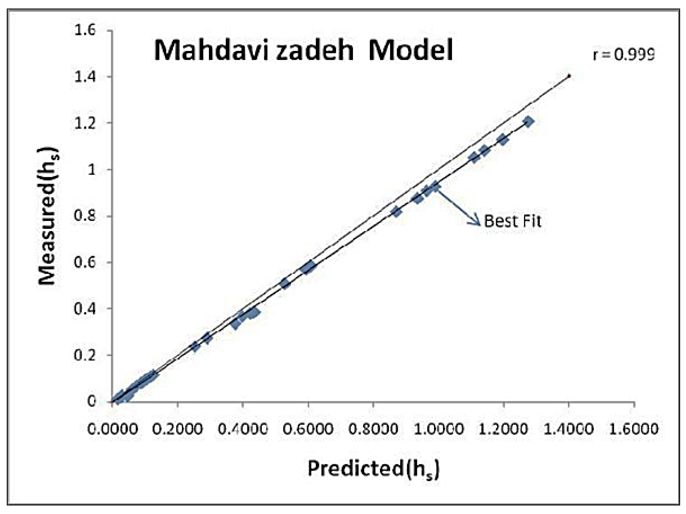
Figure 11.
Performance of the modified DOT model in estimating the height of the scour hole in the network with ten neurons in the hidden layer
Figure 11.
Performance of the modified DOT model in estimating the height of the scour hole in the network with ten neurons in the hidden layer
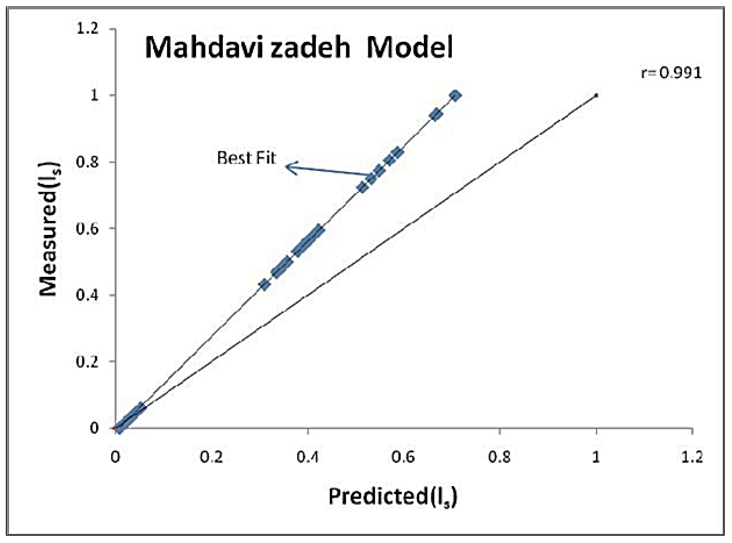
Figure 12.
Performance of the modified DOT model when estimating the length of the scour hole in the network with ten neurons in the hidden layer.
Figure 12.
Performance of the modified DOT model when estimating the length of the scour hole in the network with ten neurons in the hidden layer.
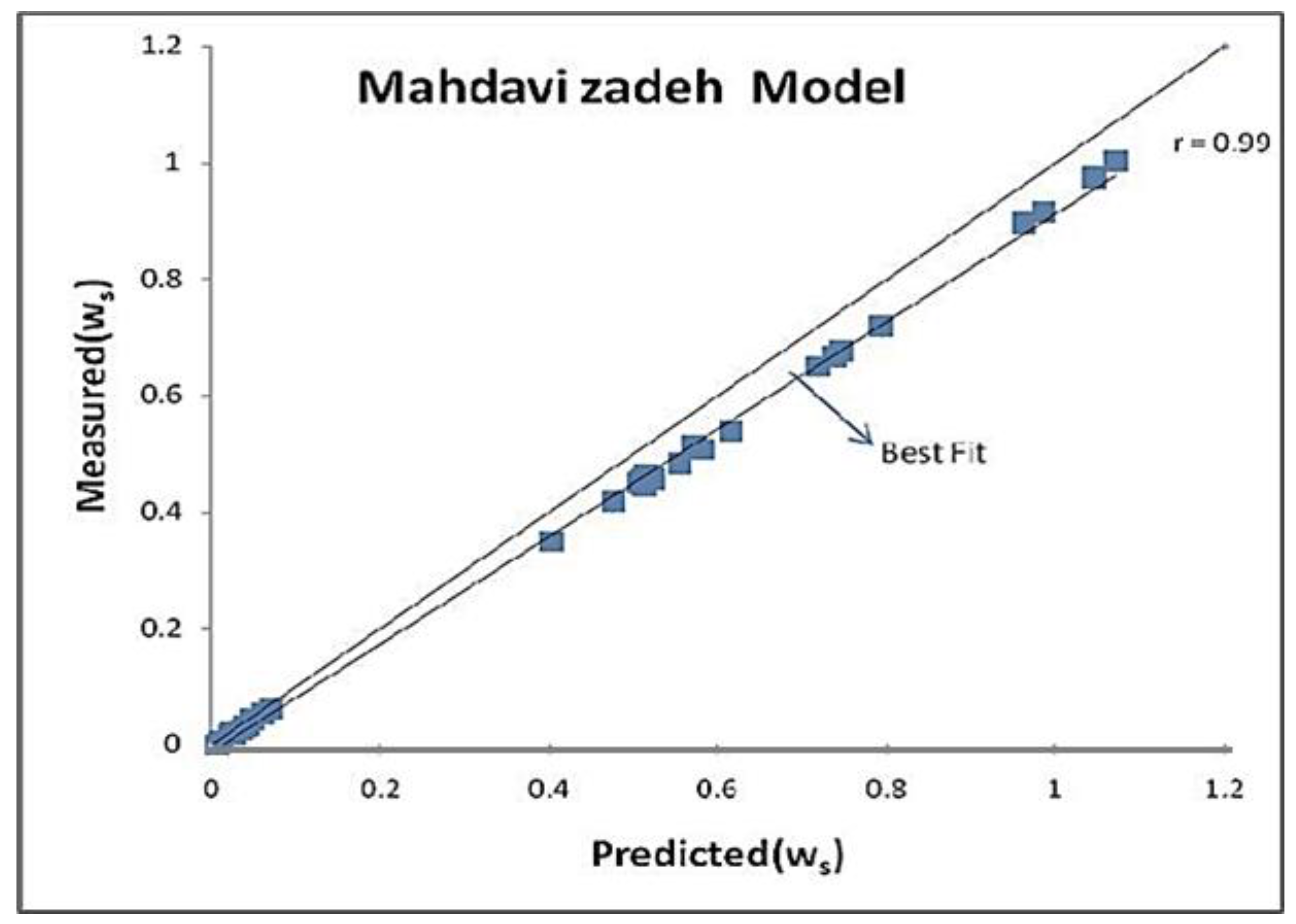
Figure 13.
Performance of the modified DOT model when estimating the width of the scour hole in the network with ten neurons in the hidden layer.
Figure 13.
Performance of the modified DOT model when estimating the width of the scour hole in the network with ten neurons in the hidden layer.
Table 1.
Network specifications
Table 1.
Network specifications
| Network Type | Educational Function | Learning Function | Execution Function | Transfer Function of First Layer | Transfer Function of Second Layer |
|---|
| Feed-forward back propagation | TrainLM | Learngdm | MSE | Tansig | Purelin |
Table 2.
Problem inputs and data range in the dimensional model.
Table 2.
Problem inputs and data range in the dimensional model.
| Problem Inputs | Q | Tw | Hc | Rc | t |
|---|
| Data range before normalization | 1.02–1.77 | 6–18 | 35–65 | 0.01–0.075 | 5–300 |
| Problem objectives | hs | Ls | ws |
| Data range before normalization | 0.05–0.2 | 0.29–1.1 | 0.27–0.72 |
Table 3.
Verification indicators of the dimensional model for estimating the depth of the scour hole in networks with one and ten neurons in the hidden layer.
Table 3.
Verification indicators of the dimensional model for estimating the depth of the scour hole in networks with one and ten neurons in the hidden layer.
| Verification Indicator | For 1 Neuron | For 10 Neurons |
|---|
| r | 0.888 | 0.9020 |
| RMSE | 0.171 | 0.16 |
Table 4.
Verification indicators of the dimensional model to estimate the length of the scour hole in networks with one and ten neurons in the hidden layer
Table 4.
Verification indicators of the dimensional model to estimate the length of the scour hole in networks with one and ten neurons in the hidden layer
| Verification Indicator | For 1 Neuron | For 10 Neurons |
|---|
| r | 0.779 | 0.9270 |
| RMSE | 0.3 | 0.263 |
Table 5.
Verification indicators of the dimensional model when estimating the width of the scour hole in networks with one and ten neurons in the hidden layer.
Table 5.
Verification indicators of the dimensional model when estimating the width of the scour hole in networks with one and ten neurons in the hidden layer.
| Verification Indicator | For 1 Neuron | For 10 Neurons |
|---|
| r | 0.765 | 0.8670 |
| RMSE | 0.213 | 0.219 |
Table 6.
Problem inputs and data range in the dimensionless model with all input parameters.
Table 6.
Problem inputs and data range in the dimensionless model with all input parameters.
| Problem Inputs | | | |
|---|
| Data range before normalization | 211.4037–40,547.97 | 0.0158–0.9494 | 0.0923–0.5143 |
| Problem objectives | | | |
| Data range before normalization | −3337.0–16.666 | −3.867–1.667 | −766.3–60 |
Table 7.
Verification indicators of the dimensionless model for estimating the height of the scour hole in networks with one and ten neurons in the hidden layer.
Table 7.
Verification indicators of the dimensionless model for estimating the height of the scour hole in networks with one and ten neurons in the hidden layer.
| Verification Indicator | For 1 Neuron | For 10 Neurons |
|---|
| r | 0.954 | 0.954 |
| RMSE | 0.18 | 0.101 |
Table 8.
Verification indicators of the dimensionless model for estimating the length of the scour hole in networks with one and ten neurons in the hidden layer.
Table 8.
Verification indicators of the dimensionless model for estimating the length of the scour hole in networks with one and ten neurons in the hidden layer.
| Verification Indicator | For 1 Neuron | For 10 Neurons |
|---|
| R | 0.975 | 0.977 |
| RMSE | 0.261 | 150.2 |
Table 9.
Verification indicators of the dimensionless model for estimating the width of the scour hole in networks with one and ten neurons in the hidden layer.
Table 9.
Verification indicators of the dimensionless model for estimating the width of the scour hole in networks with one and ten neurons in the hidden layer.
| Verification Indicator | For 1 Neuron | For 10 Neurons |
|---|
| r | 0.96 | 0.967 |
| RMSE | 0.133 | 720.1 |
Table 10.
Problem inputs and data range in the dimensionless model (considering the discharge and time)
Table 10.
Problem inputs and data range in the dimensionless model (considering the discharge and time)
| Problem Inputs | |
|---|
| Data range before normalization | 211.4037–40,547.97 0.0158–0.9494 |
| Problem objectives | | | |
| Data range before normalization | −3337.0–16.666 | −768.3–91.667 | −766.3–60 |
Table 11.
Verification indicators of the dimensionless model when estimating the height of the scour hole in the network with one neuron in the hidden layer (Inputs: discharge and time).
Table 11.
Verification indicators of the dimensionless model when estimating the height of the scour hole in the network with one neuron in the hidden layer (Inputs: discharge and time).
| Verification Indicator | For 1 Neuron |
|---|
| r | 0.867 |
| RMSE | 0.18 |
Table 12.
Verification indicators of the dimensionless model when estimating the length of the scour hole in the network with one neuron in the hidden layer (Inputs: discharge and time).
Table 12.
Verification indicators of the dimensionless model when estimating the length of the scour hole in the network with one neuron in the hidden layer (Inputs: discharge and time).
| Verification Indicator | For 1 Neuron |
|---|
| r | 0.972 |
| RMSE | 0.261 |
Table 13.
Verification indicators of the dimensionless model when estimating the width of the scour hole in the network with one neuron in the hidden layer (Inputs: discharge and time).
Table 13.
Verification indicators of the dimensionless model when estimating the width of the scour hole in the network with one neuron in the hidden layer (Inputs: discharge and time).
| Verification Indicator | For 1 Neuron |
|---|
| r | 0.963 |
| RMSE | 0.133 |
Table 14.
Problem inputs and data range in the dimensionless model (considering the discharge, downstream depth, and spillage height).
Table 14.
Problem inputs and data range in the dimensionless model (considering the discharge, downstream depth, and spillage height).
| Problem Inputs | |
|---|
| Data range before normalization | −211.4037–40,547.97 −0.5143–0.0923 |
| Problem objectives | | | |
| Data range before normalization | −16.666–0.7333 | −91.667–3.867 | −766.3–60 |
Table 15.
Verification indicators of the dimensionless model when estimating the depth of the scour hole in the network with one neuron in the hidden layer (Inputs: discharge, downstream depth, and spillage height).
Table 15.
Verification indicators of the dimensionless model when estimating the depth of the scour hole in the network with one neuron in the hidden layer (Inputs: discharge, downstream depth, and spillage height).
| Verification Indicator | For 1 Neuron |
|---|
| r | 0.931 |
| RMSE | 0.142 |
Table 16.
Verification indicators of dimensionless model when estimating the length of the scour hole in the network with one neuron in the hidden layer (Inputs: discharge, downstream depth, and spillage height).
Table 16.
Verification indicators of dimensionless model when estimating the length of the scour hole in the network with one neuron in the hidden layer (Inputs: discharge, downstream depth, and spillage height).
| Verification Indicator | For 1 Neuron |
|---|
| r | 0.963 |
| RMSE | 0.245 |
Table 17.
Verification indicators of dimensionless model when estimating the width of the scour hole in the network with one neuron in the hidden layer (Inputs: discharge, downstream depth, and spillage height).
Table 17.
Verification indicators of dimensionless model when estimating the width of the scour hole in the network with one neuron in the hidden layer (Inputs: discharge, downstream depth, and spillage height).
| Verification Indicator | For 1 Neuron |
|---|
| r | 0.886 |
| RMSE | 0.133 |
Table 18.
Coefficients and verification indicators of the regression model
Table 18.
Coefficients and verification indicators of the regression model
| Verification Indicators | Coefficients | Output Parameter |
|---|
| RMSE | R | c | b | a | k |
|---|
| 1.537 | 0.845 | 0.165 | 0.128 | 0.4 | 0.224 | |
| 3.181 | 0.887 | 0.03 | 0.102 | 0.389 | 0.848 | |
| 3.165 | 0.939 | −0.015 | 0.096 | 0.393 | 0.682 | |
Table 19.
Problem inputs and data range in DOT model (considering all parameters).
Table 19.
Problem inputs and data range in DOT model (considering all parameters).
| Problem Inputs | | | Ch | Cs |
|---|
| Data range before normalization | −860.8–−62.677 | −685.0–−0.978 | 1 | 1 |
| Problem objectives | | | |
| Data range before normalization | −337.3–−91.666 | −337.3–−91.666 | −456.0–−1.068 |
Table 20.
Verification indicators of the DOT model when estimating the depth of the scour hole in networks with one and ten neurons in the hidden layer.
Table 20.
Verification indicators of the DOT model when estimating the depth of the scour hole in networks with one and ten neurons in the hidden layer.
| Verification Indicator | For 1 Neuron | For 10 Neurons |
|---|
| r | 0.823 | 0.823 |
| RMSE | 0.221 | 0.222 |
| Test Statistics |
| tailed Asymp. Sig. 2- | 0.94 | 0.952 |
Table 21.
Verification indicators of the DOT model when estimating the length of the scour hole in networks with one and ten neurons in the hidden layer.
Table 21.
Verification indicators of the DOT model when estimating the length of the scour hole in networks with one and ten neurons in the hidden layer.
| Verification Indicator | For 1 Neuron | For 10 Neurons |
|---|
| r | 0.912 | 0.955 |
| RMSE | 0.197 | 0.196 |
Table 22.
Verification indicators of the DOT model when estimating the width of the scour hole in networks with one and ten neurons in the hidden layer.
Table 22.
Verification indicators of the DOT model when estimating the width of the scour hole in networks with one and ten neurons in the hidden layer.
| Verification Indicator | For 1 Neuron | For 10 Neurons |
|---|
| R | 0.920 | 0.920 |
| RMSE | 0.127 | 0.127 |
Table 23.
Problem inputs and data range in the modified DOT model (considering all parameters).
Table 23.
Problem inputs and data range in the modified DOT model (considering all parameters).
| Problem Inputs | | | Ch | Cs |
|---|
| Data range before normalization | −860.8–−62.677 | −685.0–−0.978 | −5238.0–−5.744 | 1 |
| Problem objectives | | | |
| Data range before normalization | −6685.0–16.666 | −337.3–−91.666 | 0.654–1.068 |
Table 24.
Verification indicators of the modified DOT model when estimating the depth of the scour hole in networks with one and ten neurons in the hidden layer.
Table 24.
Verification indicators of the modified DOT model when estimating the depth of the scour hole in networks with one and ten neurons in the hidden layer.
| Verification Indicator | For 1 Neuron | For 10 Neurons |
|---|
| r | 0.892 | 0.99 |
| RMSE | 0.174 | 0.30 |
| Test Statistics |
| tailed Asymp. Sig. 2- | 0.79 | 0.631 |
Table 25.
Verification indicators of the modified DOT model when estimating the length of the scour hole in networks with one and ten neurons in the hidden layer.
Table 25.
Verification indicators of the modified DOT model when estimating the length of the scour hole in networks with one and ten neurons in the hidden layer.
| Verification Indicator | For 1 Neuron | For 10 Neurons |
|---|
| r | 0.906 | 90.9 |
| RMSE | 0.158 | 60.15 |
Table 26.
Verification indicators of the modified DOT model when estimating the width of the scour hole in networks with one and ten neurons in the hidden layer
Table 26.
Verification indicators of the modified DOT model when estimating the width of the scour hole in networks with one and ten neurons in the hidden layer
| Verification Indicator | For 1 Neuron | For 10 Neurons |
|---|
| r | 0.920 | 90.9 |
| RMSE | 0.06 | 50.0 |
Table 27.
Verification indicators for dimensions of the scour hole for one and ten neurons in the hidden layer for dimensional input parameters.
Table 27.
Verification indicators for dimensions of the scour hole for one and ten neurons in the hidden layer for dimensional input parameters.
| Input Parameters | Number of Hidden Layer Neurons | hs | ls | ws |
|---|
| r | RMSE | r | RMSE | r | RMSE |
|---|
| 1 | 0.888 | 0.171 | 0.779 | 0.3 | 0.765 | 0.213 |
| 10 | 0.902 | 0.16 | 0.927 | 0.263 | 0.867 | 0.219 |
Table 28.
Verification indicators for dimensions of the scour hole for one and ten neurons in the hidden layer for dimensionless input parameters.
Table 28.
Verification indicators for dimensions of the scour hole for one and ten neurons in the hidden layer for dimensionless input parameters.
| Input Parameters | Number of Hidden Layer Neurons | | | |
|---|
| r | RMSE | r | RMSE | r | RMSE |
|---|
| | 1 | 0.954 | 0.18 | 0.975 | 0.261 | 0.960 | 0.133 |
| | 10 | 0.954 | 0.101 | 0.977 | 0.251 | 0.967 | 0.172 |
| | 1 | 0.867 | 0.18 | 0.972 | 0.245 | 0.963 | 0.13 |
| | 1 | 0.931 | 0.142 | 0.963 | 0.245 | 0.886 | 0.133 |
Table 29.
Verification indicators for dimensions of the scour hole for the regression dimensionless model.
Table 29.
Verification indicators for dimensions of the scour hole for the regression dimensionless model.
| Input Parameters | | | |
|---|
| r | RMSE | r | RMSE | r | RMSE |
|---|
| 0.854 | 1.537 | 0.887 | 3.181 | 0.939 | 3.165 |
Table 30.
Verification indicators for dimensions of the scour hole for one and ten neurons in the hidden layer for the input parameters of the DOT relationship.
Table 30.
Verification indicators for dimensions of the scour hole for one and ten neurons in the hidden layer for the input parameters of the DOT relationship.
| Input Parameters | Number of Hidden Layer Neurons | hs | ls | ws |
|---|
| r | RMSE | r | RMSE | r | RMSE |
|---|
| | 1 | 0.823 | 0.221 | 0.912 | 0.197 | 0.920 | 0.127 |
| | 10 | 0.823 | 0.222 | 0.955 | 0.196 | 0.920 | 0.127 |
Table 31.
Verification indicators for dimensions of the scour hole for one and ten neurons in the hidden layer for the input parameters of the modified DOT relationship.
Table 31.
Verification indicators for dimensions of the scour hole for one and ten neurons in the hidden layer for the input parameters of the modified DOT relationship.
| Input Parameters | Number of Hidden Layer Neurons | hs | ls | ws |
|---|
| r | RMSE | r | RMSE | r | RMSE |
|---|
| | 1 | 0.892 | 0.471 | 0.906 | 0.158 | 0.920 | 0.06 |
| | 10 | 0.99 | 0.03 | 0.99 | 0.156 | 0.99 | 0.05 |


