Article

CSO Generator—A Parsimonious Wastewater Quality Model for Combined Sewer Overflows

Aquafin NV, Dijkstraat 8, B-2630 Aartselaar, Belgium
*
Author to whom correspondence should be addressed.
Water 2023, 15(19), 3424; https://doi.org/10.3390/w15193424
Submission received: 17 July 2023 / Revised: 8 September 2023 / Accepted: 10 September 2023 / Published: 28 September 2023
(This article belongs to the Special Issue Modeling and Simulation of Urban Drainage Systems)

Abstract

:
Combined sewage overflows (CSOs) are a common consequence of heavy rainfall events and can have significant implications for water quality in receiving waterbodies. With climate change, these events are becoming more frequent and intense, placing greater pressure on aquatic ecosystems. To prevent water pollution, it is essential to utilize numerical tools to investigate, forecast, and establish control measures for CSOs. Typically, these tools involve a dynamic model for flow simulation combined with either a detailed model for pollutants or a simplified event mean concentration (EMC) calculation. However, both approaches have drawbacks: a detailed model requires extensive calibration time, while the EMC does not account for system dynamics. To overcome these issues, a novel system was developed that integrates the dynamic nature of the detailed model with the rapid calibration of the EMC. This model employs two distinct concepts for pollution modeling: one for soluble compounds and one for suspended solids. The resulting model was evaluated at multiple locations with varying hydraulic dynamics, demonstrating its potential utility at any location where a dynamic model of the sewer system is available.

1. Introduction

In a combined sewer system, the wastewater generated from households, and potentially from industries, is conveyed together with additional inflow during precipitation events. To ensure cost-effectiveness and environmental sustainability, the sewer system is designed to accommodate a limited flow at specific throttle points [1]. Under normal dry weather conditions, the flow can pass through the throttle unobstructed. However, during rainfall events, the flow rate may surpass the capacity of the throttle, leading to a backup of water in the sewer system. A combined sewer overflow (CSO) occurs to prevent the sewer system from surcharging and discharging to the streets when the rainfall intensity or duration is excessive. This results in potential environmental and health impacts.
Accurately quantifying the emissions and loads associated with combined sewer overflows is a vital aspect of planning, evaluating, and optimizing urban drainage systems. This task is complex and requires reliable modeling techniques. Detailed, distributed hydrodynamic models such as SWMM [1], Infoworks [2] or Mike [3] are commonly used to achieve high hydraulic accuracy [4]. Water quality is commonly evaluated based on the concentrations of various wastewater constituents, such as chemical oxygen demand (COD), biological oxygen demand (BOD), suspended solids (SSs), total nitrogen (TN), and total phosphorus (TP) [5]. During combined sewer overflow events, water quality can be characterized by an event mean concentration (EMC), which represents the average load divided by the average flow of the event [6]. Due to the dynamics of the system, a non-linear relationship between the load and the flow during a CSO event is observed [6,7,8], making it difficult to represent the water quality accurately using a fixed EMC value. In addition, previous studies [9,10,11] have shown that the minimum concentration during a CSO event varies for different overflow events and locations, indicating that a constant EMC value would lead to significant over- or underestimation of total emitted loads. While the EMC can be determined for each event, the result is only valid for that specific location and rain event. Therefore, water quality at CSO locations can only be properly characterized through monitoring at high temporal resolution [12,13,14,15].
The use of dynamic models for estimating water quality at CSO locations requires a sound basis of monitoring data for calibration. To develop and calibrate dynamic models, it is essential to have a complete understanding of the dynamics of the sewer system, including the different concentrations of wastewater constituents. Moreover, it involves considerable effort to calibrate the quality of wastewater simulations in a detailed modeling environment and raises questions about whether the calibration time and effort are justifiable for the simulation results. Some researchers address this issue by employing simplified models for both quantity and quality [16,17].
To address the trade-off between the effort required for wastewater quality modeling in urban drainage systems and the resulting benefits, we propose a hybrid approach that combines the strengths of both detailed hydrodynamic models and simplified wastewater quality models. This is achieved by integrating flow from a hydrodynamic model with a parsimonious wastewater quality model that has been calibrated using long-term water quality monitoring data. Conceptually, this approach is similar to the use of influent generators in the field of wastewater treatment plant modeling [16,18].

2. Materials and Methods

2.1. Case Study Area

In this work, we focused on a combined sewer system located in Limburg, in the northeast of Flanders, Belgium. There are 4 plants treating in total 78,800 people equivalent (p.e.) with 9000 to 30,000 p.e. per plant. The amount of p.e. is determined by 60 gBOD/p.e./day. A small part of the load of pollutants is linked to industrial activities. but this is considered to be negligible compared to the load from the households.

2.2. Monitoring Campaign

2.2.1. Monitoring Locations

Because of budget and time constraints, 13 monitoring locations were chosen. Multiple variables were measured at each location. All locations fulfill a set of predefined requirements, such as (i) easy accessibility with regard to road traffic, (ii) a secure location to place measuring and sampling devices, (iii) close vicinity to a throttle or pumping location where the flow is restricted in rain events, (iv) multiple different locations in each sewer system, (v) close vicinity to an overflow structure, (vi) an overflow visible in the hydrodynamic model at rain events of low to medium intensity, and (vii) electricity to power the devices. The measuring instruments were placed on a floating device to prevent them from running dry and to ensure that a usable signal was recorded also during dry weather. A measuring period of at least 1 year allowed us to investigate the long-term effects, e.g., seasonal changes.

2.2.2. Monitored Variables

The model focuses on 7 variables that either have a direct impact on the investigated values or are directly measured. These variables include:
(1)
Rainfall on the catchment surface (mm/h).
(2)
Flow in the sewer system and at the overflow, which varies due to the diurnal wastewater production, parasitic water, and rainfall (L/s).
(3)
Water level (m), which is used to calculate overflow volume using, e.g., the Poleni equation [19]—see, e.g., [20]. When there is a backup when a lower subcatchment is not emptying fast enough, levels will still reflect rainy conditions while flows drop below the detection limit.
(4)
Conductivity, a simple and reliable measurement that we found to be relatable with ammonia (µS/cm2).
(5)
Ammonia concentration (grab samples) (mg/L).
(6)
Turbidity, as a surrogate for suspended solids (mg/L).
(7)
Suspended solid concentration (grab samples) (mg/L).

2.2.3. Monitoring Devices and Storage

Flow monitoring is conducted using hydrostatic depth transducers and ultrasound Doppler velocity sensors (device: ISCO 2150). To supplement the flow monitoring data, 20 permanent pressure gauges (device: ECOLOG500 (OTT Hydromet, Kempten, Germany)) have been installed at CSO locations in collectors and/or storage tanks to measure water levels, and 15 data loggers have been set up to record level measurements in pumping stations. Although full flow monitoring is not possible at these locations due to poor velocity conditions, flows can be estimated using the wet well’s geometry, as demonstrated by [21,22]. Additionally, ammonia and suspended solids are measured (device: S::CAN ammo::lyser and S::CAN spectro::lyser(s::can, Vienna, Austria)). The data are logged every minute and transferred to a data server. To enable direct follow-up of the devices, the data are stored in a database along with such metadata as device location and maintenance information. In order to calibrate hydrodynamic models within AQUAFIN, a minimum of 2 precipitation monitoring locations were chosen, depending on the density of urbanization. For the current project, 12 tipping bucket rain gauges (device: ARG100 (Campbell Scientific Ltd, Loughborough, UK)) were installed in the study area, taking the size of the catchment into account. These gauges were selected as a cost-effective option compared to other techniques, as the loss in accuracy was deemed acceptable and allowed for a higher number of monitoring locations. They were installed on the ground at fenced company sites, such as WWTPs, pumping stations, and storage tanks. Sites were selected based on factors such as the distance from the mounting point to the site fence, any obstructions, and GPRS signal strength. Additionally, 1 min-resolution rain gauge data from an external source (www.waterinfo.be) was used to supplement the monitoring campaign data. Precipitation data from the nearest rain gauge was used for each CSO location to be modeled. More information regarding accuracy and measuring principles for these data can be obtained from the suppliers. Waterinfo is a webservice of the Flemish Government providing rainfall, discharge, and water levels forecast and rainfall monitoring data.

2.2.4. Data Preparation

The data used for calibration and validation are manually checked on a weekly basis to ensure accuracy. Afterward, the data are cleaned by examining when operators passed by, taking grab samples, and taking into account operator observations. Data are considered accurate if values before do not deviate more than 5% compared to after cleaning, or if a related sensor shows similar trend lines. Since two sensors will likely clog differently, an additional sensor is used to determine data validity. If one of the sensors is not working during a small window (less than half a day), a surrogate sensor will supply the data as long as the previous state was still valid before and after. In locations where the wastewater treatment plant is close, grab-sample data and daily averaged data are also used for data verification.

2.2.5. Hydraulic Data

The hydraulic models for all catchments have been calibrated and validated using the Infoworks ICM modeling environment. Validation has been performed using reference flow and level data for all monitoring locations in the sewer system. In addition to rain, groundwater infiltration (parasitic water) affects the sewer system. To calibrate the hydrodynamic sewer model, different flow and height measurements are used along with pump station characteristics. Parasitic water, which is difficult to quantify, can be estimated by analyzing dry weather flow, while calibration of land runoff surface can be done by analyzing different rain events—see, e.g., [22].

2.2.6. WWTP Data

During the calibration period, daily composite samples of influent and effluent flows were collected approximately every two weeks. The samples were analyzed for BOD5, COD, suspended solids, total nitrogen, Kjeldahl nitrogen, ammonia, nitrate, orthophosphate, and total phosphorus using standard methods [23]. A 0.45 µm polyester filter was used for sample filtration. The inlet water flow and water level were monitored every 30 s. The level of the influent of the WWTP was measured, and thus the water level of the overflow structure of the inlet of the WWTP was also recorded. Historical data spanning over 7 years are available for most WWTPs and integrated in the same dataset.

2.3. Modeling Concept

2.3.1. General Approach

To determine the amount of pollutants discharged from a combined sewer overflow, one can use a combination of dynamic flow measurements and a constant concentration value. This constant concentration value, known as the event mean concentration ([6,7,8]), is calculated based on historical data from various events. However, when examining data on conductivity, turbidity, ammonia, and suspended solids, it is evident that the concentration of pollutants varies significantly over time [11]. This paper provides several examples of such variations. Furthermore, it is expected that concentrations will differ across locations, as a system with a higher extraneous flow will have lower pollutant concentrations compared to a system without such water.
It is possible to calibrate the flow-dependent settling and resuspendable parameters and sheer stress for each separate link and node in the hydrodynamic simulation, although this approach has limitations. The number of parameters that need to be adjusted increases with the number of links and nodes, resulting in an underdetermined system and increasing the risk of overfitting the model.
We propose using available accurate dynamic flow models in combination with a simple dynamic quality model. By doing so, we can combine the accuracy and details of the dynamic model and integrate the dynamics into a simple water quality model. However, it may be necessary to invest additional time to calibrate and validate a fully detailed dynamic model with all its parameters.

2.3.2. Dissolved Compounds

Upon examining the dissolved compounds present in an ideal sewer system where each household has the same number of residents and similar surface runoff, it may be assumed that the concentration in the sewer system can be represented by Equation (1):
L P E Q P E + Q R a i n ,
where LPE denotes the load of the dissolved compound, QPE represents the flow associated with the people’s load, and QRain refers to the flow entering the sewer. All these parameters are time-dependent. Due to the dilution of rainwater throughout the entire system, the load should remain constant and equal to the load under dry weather conditions. However, in reality, this is not the case, as occasional high loadings, known as the first flush [24], occur at the beginning of a rain event. This phenomenon can be attributed to the difference in the time it takes for the concentration to drop compared to the rise in flow, resulting in an additional peak load at the start of the rain and a smaller load at the end of the rain.
In our model, the first step involves determining the dry weather concentration of pollutants from households. This concentration is then subjected to dilution caused by parasitic water and rainwater. In reality, parasitic water and rainwater contain additional pollutants, but these are not taken into account in the model. A time delay (lag) might occur due to the large volume of the sewer system relative to the flow, resulting in a smoothing effect on the concentration. The level is used to ascertain whether it is in a dry weather state or a rainy weather state. When the system is in a dry weather state, the concentration gradually returns to the dry weather levels. A schematic overview is shown in Figure 1.
The model employs four inputs and nine parameters. The inputs comprise the following:
  • Smoothed rainfall (mm/h), which accounts for the volume of water flowing into the sewer, and consequently, the target concentration within the sewer.
  • Water level (m), which determines whether the system has returned to dry weather conditions.
  • Flow (L/s).
  • Parasitic flow, which is used to determine dry weather dilution (L/s).
The parameters, on the other hand, are:
  • A dry weather concentration (mg/L) (used in cases of no parasitic water), which is determined by the average load and flow of the households. The load and flow can be determined from the average load of the WWTP.
  • The dry weather level (m). Below this level, there is no runoff effect anymore of any rain into the sewer. This parameter is dependent on the amount of parasitic water in the system.
  • A daily wastewater profile. A sinus profile characterized by an amplitude and a phase shift (radians). Some authors [25] suggest using a combination of two sinus functions with several parameters.
  • The equation used for the incoming time-dependent dry weather concentration at each node in the sewer system is represented as y = C_dry × (1 + ap sin(t/2pi + bp)), where y is the concentration, C_dry denotes the average dry weather concentration (mg/L), and ap and bp represent the two fitting parameters for the sinusoidal function.
  • A rain factor (h/mm): to determine how much dilution comes from 1 mm of rain by using the following equation: C = C_dry × (1/(1 + rain factor × rain)). This parameter is related to the size of the runoff surface.
  • A rain-dependent time delay (2 parameters: time-lag DWA and time-lag RWA (d)). This determines the time between the start of the rain and the reaction on the incoming concentration.
  • The logistic function (2 parameters: c_logDWA and c_logRWA (1/d)). Our model incorporates a function that accounts for the time delay between the incoming concentration of pollutants in the sewer and the concentration at a specific location. This function also enables a smooth transition from the original concentration to another through an exponential curve. The time-dependent concentration equation utilized for this purpose is as follows: y = 1/(1 + exp(−1 × (t − b)/c_log)). The parameter c_log, which influences the steepness of the transition, is dependent on the rain, the flow rate, and the level within the sewer system.

2.3.3. Suspended Solids

A portion of the suspended solids is in motion and can be modeled with the same equations used for the dissolved compounds. However, the remaining settleable and resuspendable fraction requires an extension to the model. Under low flow conditions, all settleable particles will settle, whereas at higher flow rates, more particles will be in motion. At the peak flow, the maximum number of particles will remain in suspension. Subsequent to the decrease in flow, a greater proportion of particles will settle. Due to the characteristic rise to a maximum followed by a return to normal, it is presumed that the prevailing time-dependent function follows a Gaussian function (see Equation (2)). The width of this Gaussian function (parameter c in Equation (2)) is dependent upon the size and retention time of the sewer system, while the amplitude (parameter a in Equation (2)) depends on the time interval between rainfall events and the cessation of the preceding rain. The parameter t0 denotes the mid time of the flush and is dependent on the beginning of the rain and the rain duration.
c o n c e n t r a t i o n t = a e t t 0 2 2 c 2 ,
The intensity of rain affects the amount of water entering the sewer system, which in turn increases the velocity and resuspends a higher load of particles. The amount of resuspended particles is set to be linearly dependent on the flow, which is a first-order approximation of the more complex relationship of reality. Meanwhile, the accumulation of solids is influenced by the time between rain events, with longer intervals resulting in more solids accumulating. As more solids settle, the wet section in the pipe decreases and the velocity increases, which makes it harder for the solids to settle and the increase in solids starts to level out. The increase in accumulation rate is modeled with a simple square-root dependence on the time between the current and previous rain, similar to other studies [26].

2.3.4. Model Calibration

To establish the CSO model, certain initial information is required for each location:
  • Firstly, we need to identify the pipe in the trunk sewer (LCSO) where we can assume that the pollutant concentrations at the CSO will be similar to the concentrations at the LCSO. When this LCSO is close to a pumping station, the incoming pipe to the pumping station was chosen as LCSO because during dry weather the levels are as high as during wet weather. Before making this assumption, it is important to check for any differences between overflow and carry-on concentrations. For the locations discussed in this paper, any discrepancies between concentrations at LCSO and at CSO locations were assumed as negligible due to the short distance between the CSO and the LCSO and the small size of the CSO chambers.
  • Secondly, the dry weather and parasitic flow and daily dry weather profile at the LCSO location must be known. This can be either determined by a measuring campaign or by a full dynamic model.
  • Finally, the daily average pollutant load at the LCSO location must be determined, either through measuring campaigns or by deducing it from WWTP daily average loads and related people equivalent. If these data are not available, general patterns or design values from a WWTP can be used.
The above information will be used for the calibration of the CSO generator, following these major steps, which will be explained in detail below:
  • Determine the dry weather flow logistic function parameter for soluble compounds.
  • Determine the full set of parameters for soluble compounds.
  • Determine all additional parameters for suspended solids compounds.
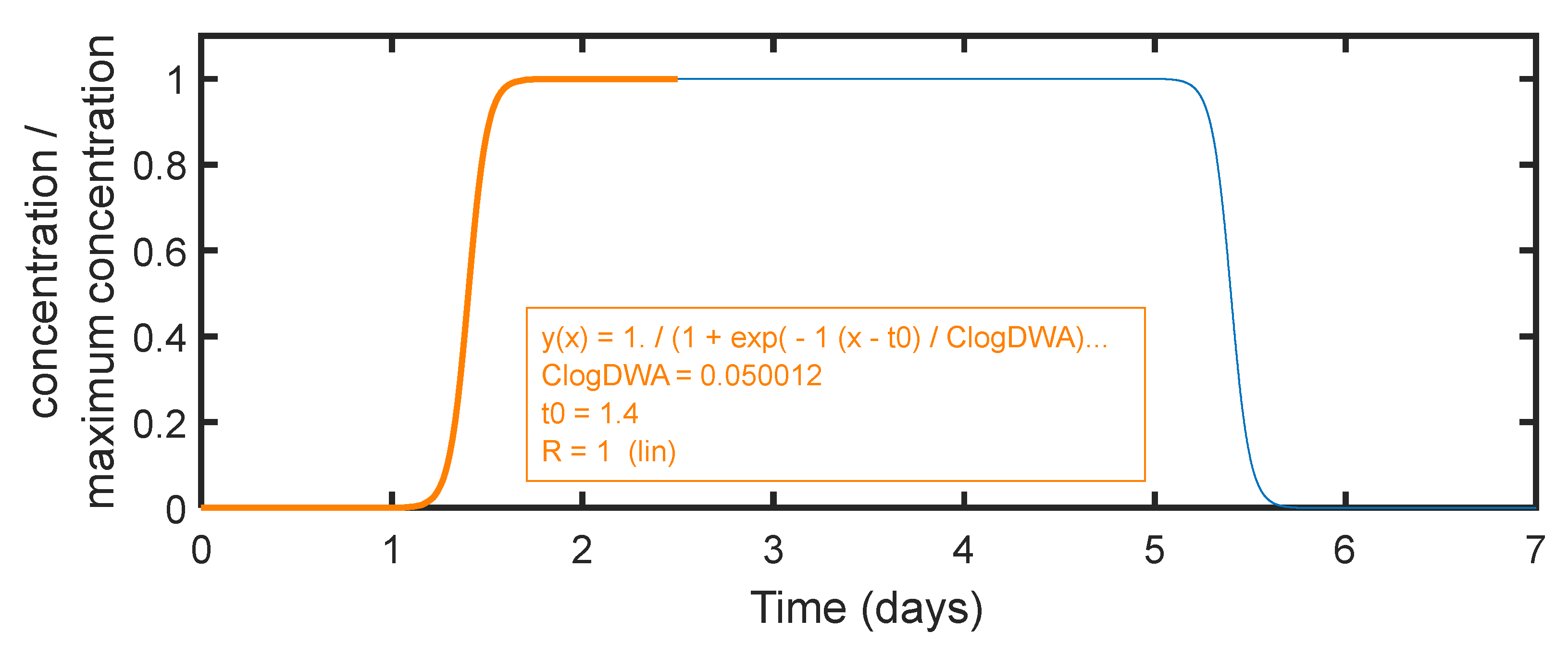
To acquire C_logDWA, a fixed general pollutant is used in the model, and the sewer system is analyzed by keeping the flow constant and alternating the general pollutant on a weekly basis. Specifically, the concentration of NH4+ (or a similar non-settleable compound) is set to 0 mg/L for 2 days and then set to 1000 mg/L for 5 days. This process is repeated on a weekly basis. This alternating concentration simulates the concentration build-up that occurs during dry weather. The concentration data are then used to determine the C_LogDWA by analyzing the steepness and shape of the increasing and decreasing concentration as a function of the time. A mean squared error on the concentration is used for the calibration. The C-LogDWA is only one parameter that needs to be determined in the calibration process. An example can be seen in Figure 2.
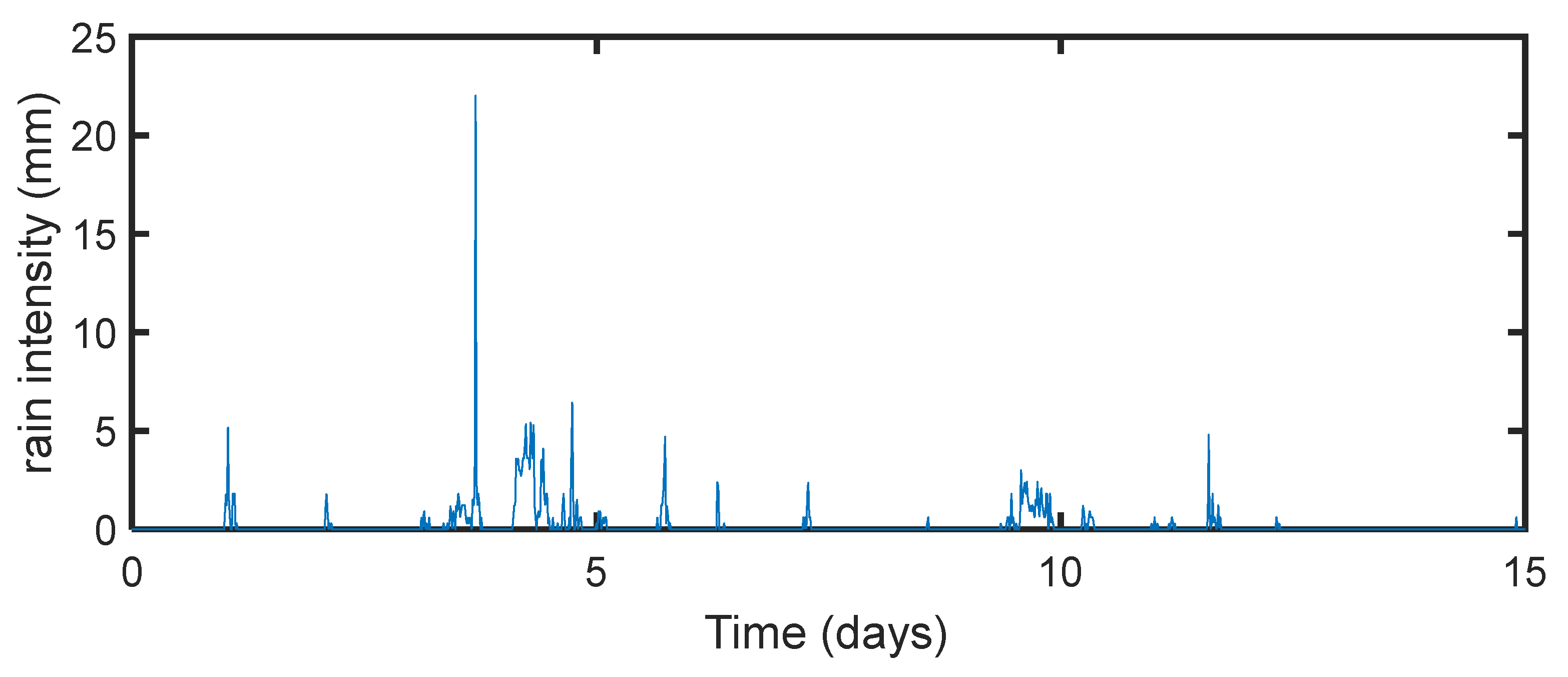
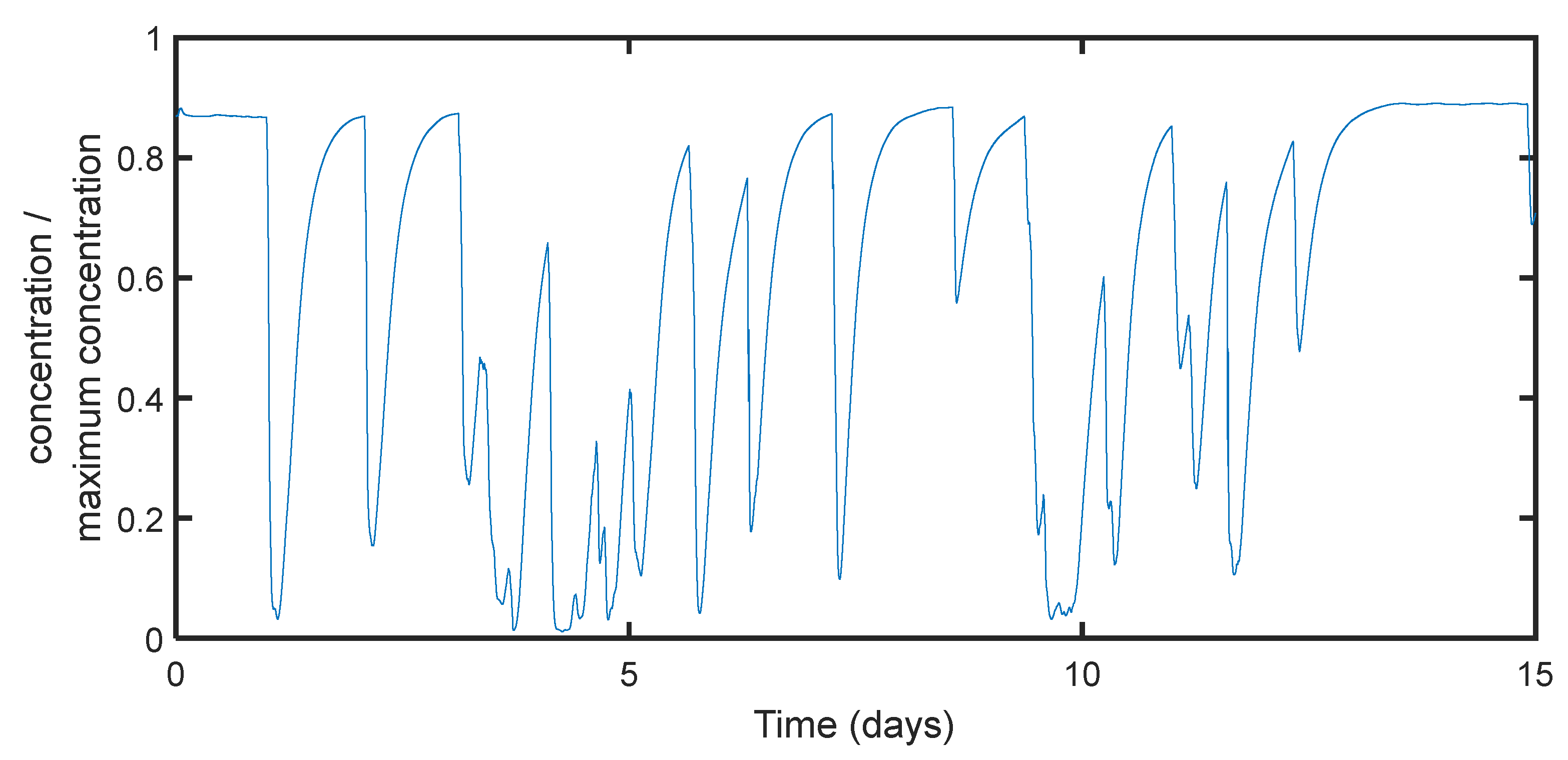
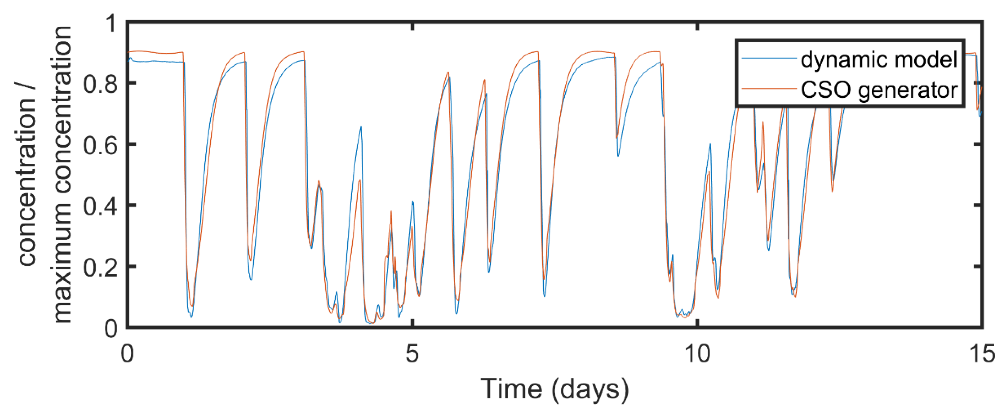
In the second step of the calibration process, the previously determined C_logDWA factor is utilized as input. This step involves the use of the NH4+ concentration (any soluble compounds would suffice) data obtained from 15 days’ hydrodynamic simulation, which is based on a specific rainfall pattern (as shown in Figure 3). The rainfall pattern consists of dry periods as well as periods of varying rainfall intensity, which help to characterize the transition between different states of the sewer system and to determine the rain dependency of certain parameters. The rainfall data set is taken as a subset from real rainfall data at Ukkel, Belgium. By examining multiple systems and multiple locations over a full year simulation, only a fit on this arbitrary 15 day period was necessary to determine the model parameters. An illustration of the normalized concentration of one location in the hydrodynamic model is provided in Figure 4. In this figure, a fixed dry weather load is used. A time-dependent dry weather load resembles more reality. In this paper we have chosen a 2-step approach to first fit the concentration with a fixed dry weather load and afterwards do a fit with a time-dependent dry weather load. A fit on the concentration can be performed using a mean absolute error, based on the previously determined DWA value and the available data. A mean absolute error enables us to focus the fit more on the low values compared to the mean squared error.
In the final step, the suspended solids concentration model uses the previously determined soluble compound parameters in combination with fixed values for additional parameters, which will be selected based on fitting past suspended solid data or prior knowledge. By using this system, the NH4+ and suspended solid concentrations can be determined. If the reader wants to generate, for example, the BOD concentration, one still must deduce a relationship between the BOD and NH4+ and suspended solids (for example WWTP measurements) and use these to determine the time-dependent values.

3. Results

In the subbasins mentioned above, there are multiple CSOs. The results shown in this paper are taken at arbitrary locations. Similar results could be seen and conclusions could be taken when a different location would have been chosen. In the paper, we focus on the concentrations at the LSCO because they will in a later stage be combined with the flow of the CSO.

3.1. NH4+ Concentration

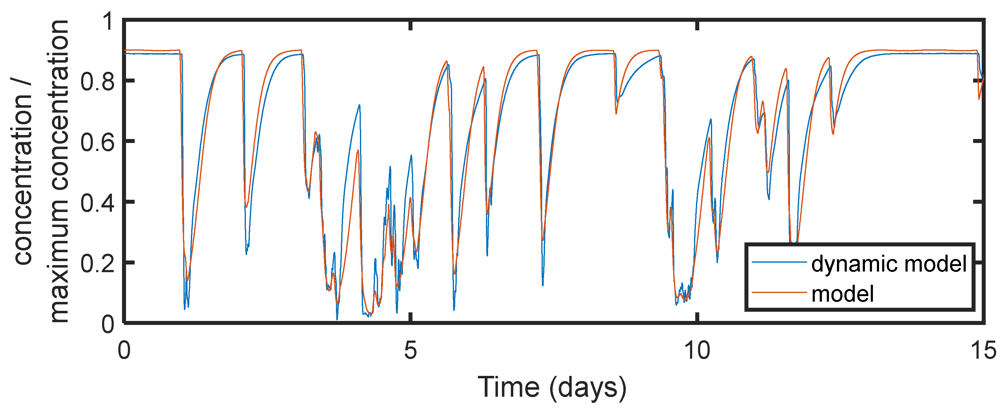
The scaled concentration of NH4+ as a function of time is presented for one random location in Figure 5 for both the hydrodynamic model and the new CSO model. The rainfall used as input is shown in Figure 3. The concentration drops when rainfall runoff enters the sewer system, due to dilution. During heavier rainfall events, the concentration drops lower compared to lighter rainfall events. After the rainfall event ends, the concentration gradually rises to the dry weather concentration, which typically takes around 0.5–1 day. In most subcatchments in Flanders, the hydraulic retention time during dry weather is around 6–24 h; therefore, a gradual rise in concentration is expected for this duration. The Nash–Sutcliffe efficiency (NSE) of 0.93 indicates that the model provides a good representation of the data. Literature suggests that a NSE above 0.6 is considered a good fit [27]. The root mean squared error (RMSE) is 0.06.
In Figure 6, the scaled concentration in another location is presented and a NSE of 0.96 and an RMSE of 0.06 is observed, indicating good agreement between the model results and the measurements. Similar results were obtained for various other locations.

3.2. NH4+ Load

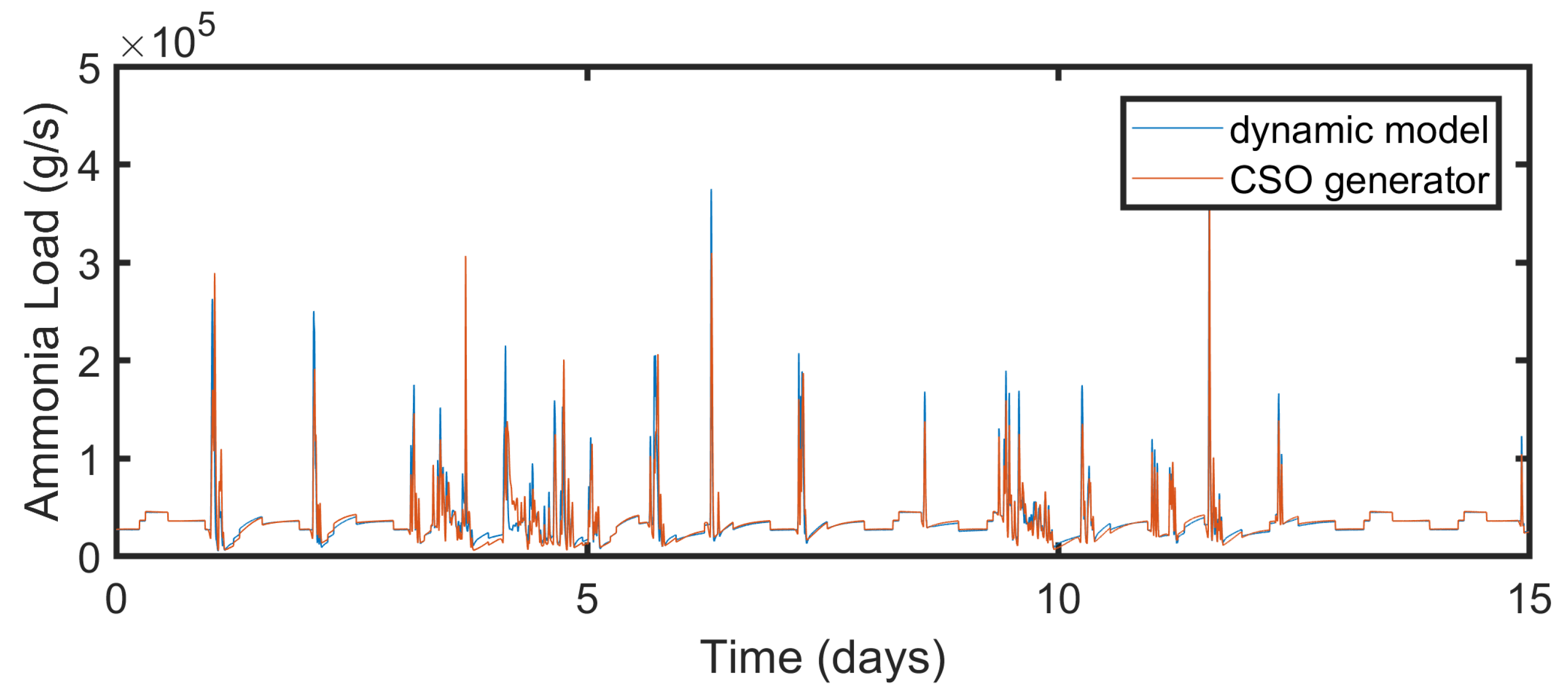
Figure 7 shows a comparison between the load of ammonia according to the existing hydrodynamic model and the load after the new model. The Nash–Sutcliffe efficiency (NSE) for this fit is 0.65 and a RMSE of 14 × 103 g/s. For location 2, the NSE of the load is 0.76 and a RMSE of 17 × 103 g/s. The rainfall series used in the simulation consists of more dry weather periods than rainy periods. Therefore, the calibration will also be more suited for situations with predominantly dry weather. However, the load is mainly determined during the first flush moments, which occur during rainy periods, as the load during this time is almost 10 times higher than during dry weather. Thus, even small deviations in concentration during the first flush moments can significantly affect the load. Hence, the NSE for the load is slightly lower when using the concentration calibration. If the focus is on peak loads in the sewer system, a specific model fit could be performed using the load instead of the concentration. This would result in a higher NSE for the load, but a lower NSE for the concentration, depending on whether the user wants to put more emphasis on the load or on the concentration. In this paper, more emphasis has been given to the concentration as it will be combined with the flow at the CSO location.
As shown in Figure 7, load peaks of ammonia up to nine times the dry weather load can occur, which is consistent with other references [24]. This peak is only visible for a short period of time, typically a few hours, after which the load becomes the same as the dry weather load. When a peak load is observed, it could be assumed that it comes from an extra external source. However, in the hydrodynamic model, there is no such extra load. The first flush occurs due to the delay in concentration compared to the flow. The peak value depends on the location, but a peak of up to 10 times the dry weather concentration seems to occur in most systems investigated. The higher the rain intensity after a dry weather period, the higher the flushing effect.
The peak is also lower when the system is still not yet in full dry weather conditions after the previous rain, which can be observed when comparing around day 12 (long dry weather period) with around day 4.75 (directly after rain period), where the rain (see Figure 3) almost looks similar, but peak loading is much higher around day 12.

3.3. Conductivity

Figure 8 displays the conductivity load data for a location in Eksel. In this study, we found that the concentration of soluble compounds can be extended to non-dissolved compounds for the suspended solids using fixed parameters for flushing of the suspended solids. The dissolved compound part of the CSO generator model is used for conductivity since in the paper it is assumed that only a small part of conductivity comes from suspended solids, and the effect of suspended solids on conductivity is minimal, which is seen by the fit of the CSO model. The model fits well for conductivity, with a Nash–Sutcliffe efficiency (NSE) of 0.71 and an RMSE of 1.7 × 10³ g/h over the whole period. The results shown are only for the period between 7 February 2018 and 22 March 2018 and were obtained using a single point (non-corrected) rainfall. The model results show good agreement with the dry weather profile and also during the rain peaks. As seen in previous hydrodynamic model results, peak values are about one order of magnitude higher than during dry weather periods, and this is still observed even for dissolved compounds. Therefore, the time difference between flow and concentration suggested by Krebs [24] is confirmed by these results. A slight difference between the model and the data is observed around 4 March 2018. Because the rain is non-corrected rainfall data, differences between reality and the rain data are possible. When a peak occurs in a different time or a different peak intensity, this could vary the model results. This could result in fewer peaks in the loading due to a smaller time lag between the concentration and flow. Alternatively, an increased conductivity observed could be due to the degradation of suspended solids to soluble compounds in the sewer or due to deicing salt or any other extra ions, although the authors were unable to distinguish between these possibilities.

3.4. Suspended Solids

Figure 9 displays the suspended load data for the same location as Figure 8. The CSO model was expanded to incorporate suspended solids, using the mean concentration and peak dry weather factor of the dry weather profile. Fixed values were selected for the fitting parameters of suspended solids, mainly accounting for flush effects from settling and resuspension. Visual analysis suggests a good match, but the Nash–Sutcliffe efficiency (NSE) is below 0.1, indicating poor fit. The discrepancy between visual and NSE evaluations is likely due to a last effect that was not considered in the model. Specifically, some solids remained settled in the main trunk after the rain, and as the water level in the main trunk dropped and water speed increased, these solids were resuspended, leading to a so called last flush effect. This effect was not accounted for in the new model, explaining the low NSE despite the apparent visual agreement. Refs. [28,29] describe this phenomenon.
On approximately 4 March 2018, it appears that the “first” flush was smaller than expected. This could be explained by the lower rain intensity on the subcatchment compared to what was actually observed. A higher rain intensity would have a greater flushing effect, leading to a larger first flush. The fact that both the conductivity and suspended solids were not fully flushed out around this time suggests that higher rain intensity may be a contributing factor, because with a higher rain intensity, more suspended solids flush out in the model of the suspended solids.
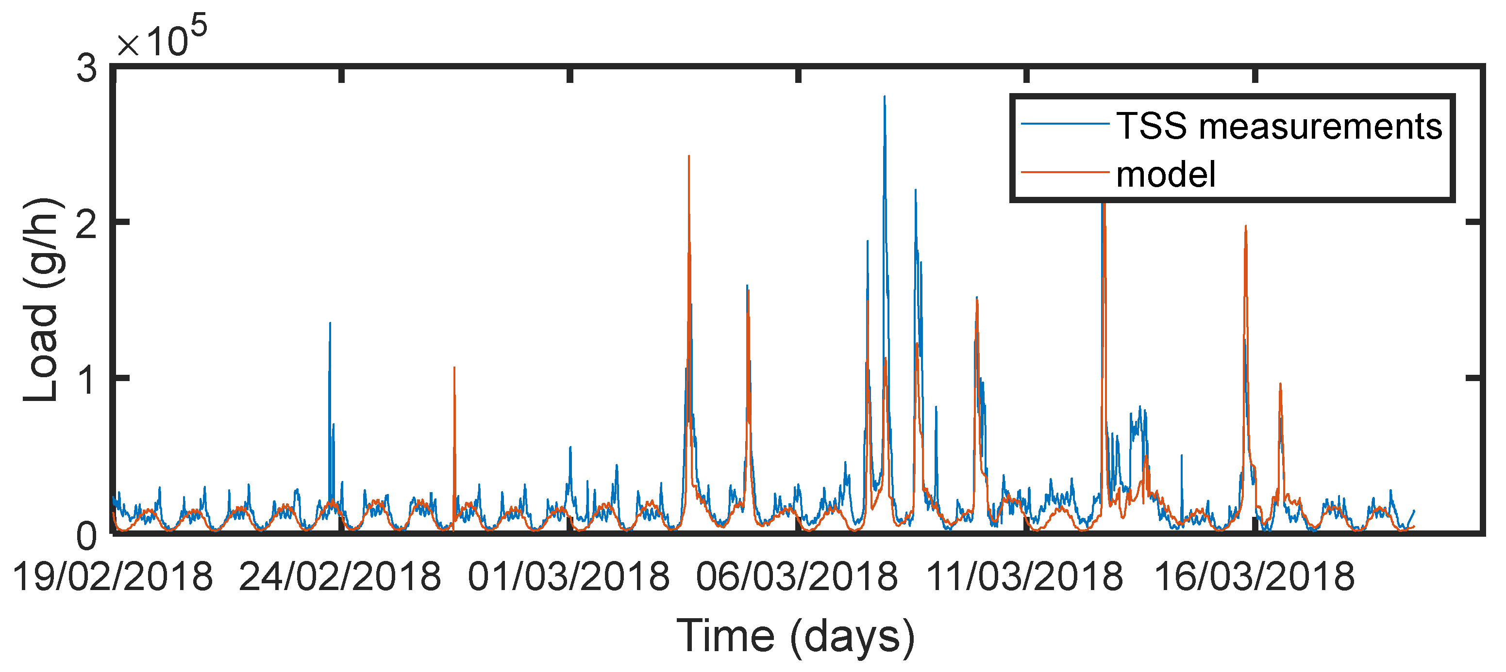
Figure 10 displays the load of suspended solids at a location in Peer, and the model appears to provide a good representation of the data. However, some discrepancies are observed, such as a TSS load peak on 24 February 2008 despite no measured rain within two days, and a rain peak on 27 February 2008 without a corresponding TSS peak. These differences may be due to small variations in the rain falling on the subcatchment compared to the measured rain, since the rain measurement used is close but not exactly on the location. No data points were removed in the data analysis, and only the average was taken. Another problem arises on 13 March 2018, where the TSS signal remains high, despite only a small increase seen in the model. This constant high value is likely due to dirt sticking to the meter, which is removed at the end of the event when velocities are higher as the system empties.
Additionally, it is observed that the DWA profile does not match exactly a simple sinus function does well enough. The Nash–Sutcliffe efficiency (NSE) is 0.43 and an RMSE of 16 × 103 g/h, indicating moderate agreement between the model and data, with good visual agreement. The absence of a last flush effect in this data leads to a better fit than seen in the Eksel case. Further data cleaning would likely resolve the deviation around 13 March 2018 and result in a higher NSE. Overall, the results of the model of the suspended solids show a bigger error because there is a big dependency of the suspended solid peaks on the rain. Furthermore, in our dataset the measurements of suspended solids were more susceptible to error due to clogging compared to a conductivity measurement.

4. Discussion

The architecture of the CSO generator is simple and easy to calibrate. It allows for adjusting the DWA profile as needed. The model parameters are easy to understand, calibrate, and manually adjust. The newly designed model uses data and underlying dynamics available from the hydrodynamic model, which can be used to gain extra information. The model can perform long-term simulations without requiring extra time, as a 15-day time period is enough to determine the model’s parameters for the dissolved compound. After calibration, the model can run in minutes, while the hydrodynamic model combined with the dissolved compounds would run for hours or even days. This way, multiple scenarios can be investigated.
Figure 5 shows that the concentration of dissolved compounds during high flows highly varies with time. A factor of 3 can be observed between the minimum concentration of different rain events. The same amount of information as an extensive EMC database can be obtained with less effort and fewer measurements. The model only needs a short well-defined rain event for calibration, which requires a low amount of calibration time. The newly designed model uses the hydrodynamic model, which incorporates the rain, parasitic water, and all other effects, to get a better estimate of the concentration in each situation without an extensive measuring campaign.
Figure 6 shows that the lowest concentration during different rain events varies. Choosing one EMC to represent all concentrations for only one overflow structure could hence lead to significant errors. The concentrations change as a function of time during the rain event. Thus, using an EMC to account for the time-dependent effect is not advisable. Extrapolating concentrations from one location to another is impossible due to variation in rain intensity and dry weather concentration due to parasitic water. Therefore, the EMC should not only depend on the rain event and location but also the amount of parasitic water. Using the EMC would only be practical if a large database could be set up that takes into account all these effects, which would require an enormous amount of time/work. Some authors [30] use a location-independent time-dependent concentration instead of an EMC. However, this time-dependent concentration does also not solve the issues stated above about the parasitic water.
The newly created model combines the high-accuracy results of the dynamic model with a simple, easy-to-calibrate gray-box model for the concentration. This allows the authors to take the full effect of all dynamics in the system into account with an easy-to-calibrate system for the quality model. This will ensure that the emissions to the river will be easier to investigate by using the already available water quantity model. The results were obtained by investigating four subcatchments located close to each other, where the topology of the urban drainage system is similar. However, extra care should be taken to investigate that the parameters for non-dissolved compounds could depend on the topology of the system. A new study close to Houthalen in Belgium is under investigation.

5. Conclusions

A new model is designed by integrating the flow from a hydrodynamic model with a parsimonious wastewater quality model that has been calibrated using long-term water quality monitoring data. The general concept of the model uses time dilation of the concentration with respect to the flow. The results of the model are near perfect compared to the hydrodynamic NH4+ results. The results of the model are comparable with the real live conductivity data. The model results have a visually good fit with the suspended solids data, but some deviations are still present due to inaccurate rain data or due to a last flush effect. The latter is not yet incorporated in the newly designed model. In this paper, a new model is thus presented that integrates both the dynamic behavior of the detailed hydrodynamic models and a rapid calculation.

Author Contributions

Conceptualization, methodology and original draft preparation: T.W.; visualization, review and editing: S.K.; review and editing: R.D.; review and editing and funding acquisition: J.V.A. All authors have read and agreed to the published version of the manuscript.

Funding

This research was partially funded by Interreg Vlaanderen-Nederland, European Fund for Regional Development, under the project IMPAKT!

Data Availability Statement

The data presented in this study are available on request from the corresponding author.

Conflicts of Interest

The authors declare no conflict of interest. The funders had no role in the design of the study; in the collection, analyses, or interpretation of data; in the writing of the manuscript, or in the decision to publish the results.

References

  1. Rossman, L.A. Storm Water Management Model: User’s Manual, Version 5.0; United States Environmental Protection Agency: Cincinnati, OH, USA, 2005.
  2. Innovyze. InfoWorks Integrated Catchment Modeling (ICM), Version 8.5.5; Innovyze: San Francisco, CA, USA, 2018. [Google Scholar]
  3. DHI. MIKE+Collection System User Guide; DHI: Shenzhen, China, 2023. [Google Scholar]
  4. Vezzaro, L.; Grum, M. A Generalised Dynamic Overflow Risk Assessment (DORA) for Real Time Control of Urban Drainage Systems. J. Hydrol. 2014, 515, 292–303. [Google Scholar] [CrossRef]
  5. Koot, A.C.J. Behandeling van Afvalwater; 2e ongew. en uitgebr. dr.; Waltman: Delft, The Netherlands, 1982; ISBN 978-90-212-3076-4. [Google Scholar]
  6. Lee, J.H.; Bang, K.W. Characterization of Urban Stormwater Runoff. Water Res. 2000, 34, 1773–1780. [Google Scholar] [CrossRef]
  7. Kabbani, M.S. Using PCSWMM to Simulate First Flush and Assess Performance of Extended Dry Detention Ponds as Structural Stormwater BMPs in a Large Polluted Urban Watershed. Ph.D. Thesis, University of Iowa, Iowa City, IA, USA, 2015. [Google Scholar]
  8. Kang, J. Modeling First Flush and Particle Destabilization: Implications for Design and Operation of Stormwater BMPs; University of California: Los Angeles, CA, USA, 2005; Volume 174. [Google Scholar]
  9. Di Modugno, M.; Gioia, A.; Gorgoglione, A.; Iacobellis, V.; la Forgia, G.; Piccinni, A.; Ranieri, E. Build-Up/Wash-Off Monitoring and Assessment for Sustainable Management of First Flush in an Urban Area. Sustainability 2015, 7, 5050–5070. [Google Scholar] [CrossRef]
  10. Kim, L.-H.; Jeong, S.-M.; Ko, S.-O. Determination of First Flush Criteria Using Dynamic EMCs (Event Mean Concentrations) on Highway Stormwater Runoff. Water Sci. Technol. 2007, 55, 71–77. [Google Scholar] [CrossRef] [PubMed]
  11. Leutnant, D.; Muschalla, D.; Uhl, M. Stormwater Pollutant Process Analysis with Long-Term Online Monitoring Data at Micro-Scale Sites. Water 2016, 8, 299. [Google Scholar] [CrossRef]
  12. Gamerith, V.; Muschalla, D.; Veit, J.; Gruber, G. Online Monitoring of Combined Sewer Systems: Experiences and Application in Modeling. J. Water Manag. Model. 2011. [Google Scholar] [CrossRef]
  13. Gruber, G.; Bertrand-Krajewski, J.-L.; Beneditis, J.D.; Hochedlinger, M.; Lettl, W. Practical Aspects, Experiences and Strategies by Using UV/VIS Sensors for Long-Term Sewer Monitoring. Water Pract. Technol. 2006, 1, wpt2006020. [Google Scholar] [CrossRef]
  14. Lepot, M.; Torres, A.; Hofer, T.; Caradot, N.; Gruber, G.; Aubin, J.-B.; Bertrand-Krajewski, J.-L. Calibration of UV/Vis Spectrophotometers: A Review and Comparison of Different Methods to Estimate TSS and Total and Dissolved COD Concentrations in Sewers, WWTPs and Rivers. Water Res. 2016, 101, 519–534. [Google Scholar] [CrossRef] [PubMed]
  15. Langergraber, G.; Fleischmann, N.; Hofstädter, F. A Multivariate Calibration Procedure for UV/VIS Spectrometric Quantification of Organic Matter and Nitrate in Wastewater. Water Sci. Technol. 2003, 47, 63–71. [Google Scholar] [CrossRef] [PubMed]
  16. Gernaey, K.V.; Flores-Alsina, X.; Rosen, C.; Benedetti, L.; Jeppsson, U. Dynamic Influent Pollutant Disturbance Scenario Generation Using a Phenomenological Modelling Approach. Environ. Model. Softw. 2011, 26, 1255–1267. [Google Scholar] [CrossRef]
  17. Gernaey, K.V.; Rosen, C.; Benedetti, L.; Jeppsson, U. Phenomenological Modeling of Wastewater Treatment Plant Influent Disturbance Scenarios. In Proceedings of the 10th International Conference on Urban Drainage, Copenhagen, Denmark, 21–26 August 2005; Volume 8. [Google Scholar]
  18. Flores-Alsina, X.; Gernaey, K.V.; Jeppsson, U. Global Sensitivity Analysis of the BSM2 Dynamic Influent Disturbance Scenario Generator. Water Sci. Technol. 2012, 65, 1912–1922. [Google Scholar] [CrossRef] [PubMed]
  19. Poleni, G. De Motu Aquae MixtoLibri Duo; Kessinger Publishing: Whitefish, MO, USA, 1717. [Google Scholar]
  20. Bollrich, G. Technische Hydromechanik—Grundlagen, Band 1, 6th ed.; Huss-Medien: Berlin, Germany, 2007; ISBN 978-3-345-00912-9. [Google Scholar]
  21. Fencl, M.; Grum, M.; Borup, M.; Mikkelsen, P.S. Robust Model for Estimating Pumping Station Characteristics and Sewer Flows from Standard Pumping Station Data. Water Sci. Technol. 2019, 79, 1739–1745. [Google Scholar] [CrossRef] [PubMed]
  22. Van Assel, J.; Kroll, S.; Delgado, R. Calculation of Dry Weather Flows in Pumping Stations to Identify Inflow and Infiltration in Urban Drainage Systems. Water 2023, 15, 864. [Google Scholar] [CrossRef]
  23. APHA. Standard Methods for the Examination of Water and Wastewater, 20th ed.; American Public Health Association: Washington, DC, USA, 1999. [Google Scholar]
  24. Krebs, P.; Holzer, P.; Huisman, J.L.; Rauch, W. First Flush of Dissolved Compounds. Water Sci. Technol. 1999, 39, 55–62. [Google Scholar] [CrossRef]
  25. Langergraber, G.; Alex, J.; Weissenbacher, N.; Woerner, D.; Ahnert, M.; Frehmann, T.; Halft, N.; Hobus, I.; Plattes, M.; Spering, V.; et al. Generation of Diurnal Variation for Influent Data for Dynamic Simulation. Water Sci. Technol. 2008, 57, 1483–1486. [Google Scholar] [CrossRef] [PubMed]
  26. Gupta, K.; Saul, A.J. Suspended Solids in Combined Sewer Flows. Water Sci. Technol. 1996, 33, 93–99. [Google Scholar] [CrossRef]
  27. Moriasi, D.N.; Arnold, J.G.; Van Liew, M.W.; Bingner, R.L.; Harmel, R.D.; Veith, T.L. Model Evaluation Guidelines for Systematic Quantification of Accuracy in Watershed Simulations. Trans. ASABE 2007, 50, 885–900. [Google Scholar] [CrossRef]
  28. Qin, H.; He, K.; Fu, G. Modeling Middle and Final Flush Effects of Urban Runoff Pollution in an Urbanizing Catchment. J. Hydrol. 2016, 534, 638–647. [Google Scholar] [CrossRef]
  29. Silvagni, G.; Volpi, F.; Celestini, R. Sediment Transport in Sewers: The Cesarina Combined Sewer Network. WIT Trans. Ecol. Environ. 2014, 182, 283–295. [Google Scholar]
  30. Dirckx, G.; Vinck, E.; Kroll, S. Stochastic Determination of Combined Sewer Overflow Loads for Decision-Making Purposes and Operational Follow-Up. Water 2022, 14, 1635. [Google Scholar] [CrossRef]
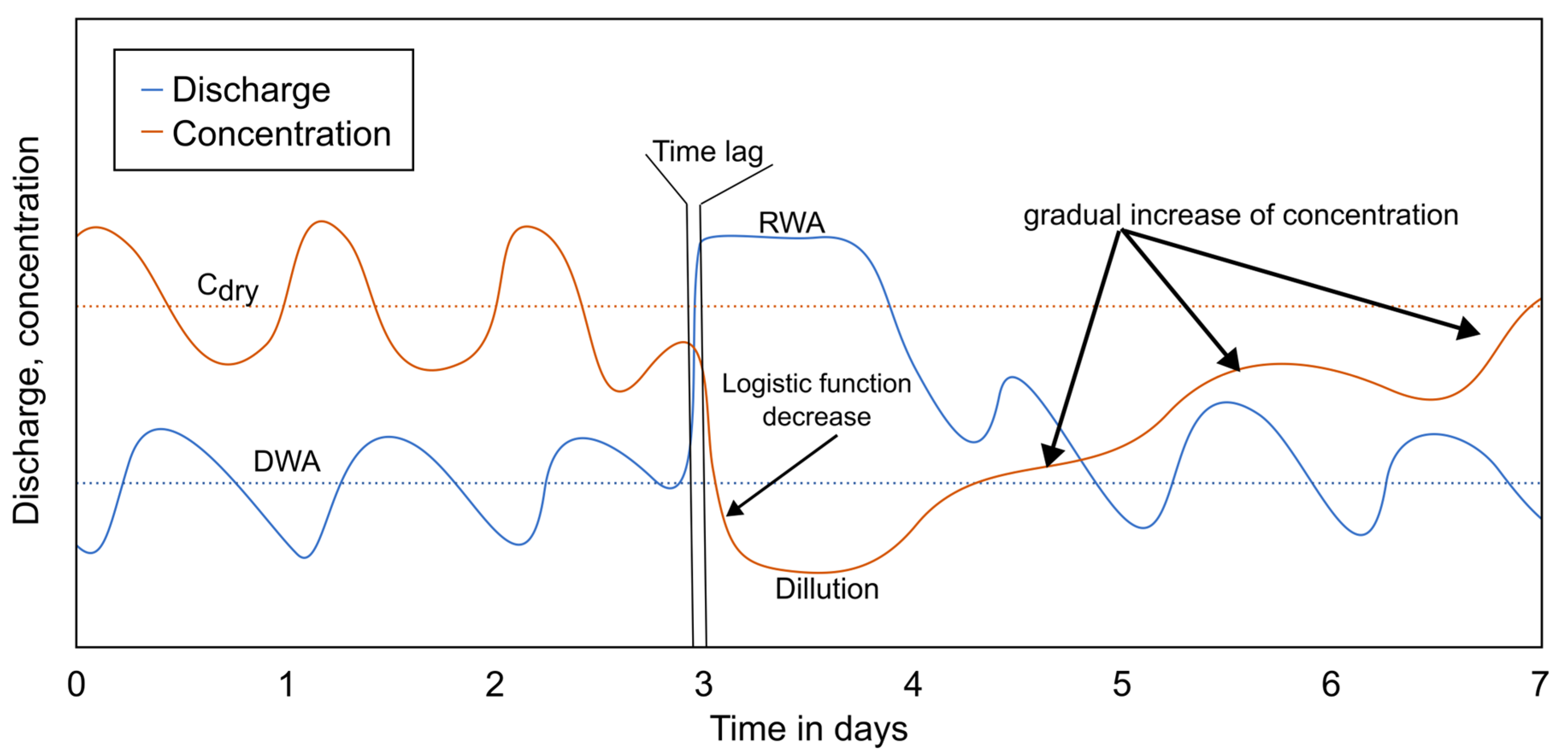
Figure 1. Schematic overview of the results of the model.
Water 15 03424 g001
Figure 2. Concentration of NH4+ as function of the time to determine the DWA factor for the logistic function (C_logDWA).
Water 15 03424 g002
Figure 3. Specific rain profile for 15 d calibration.
Water 15 03424 g003
Figure 4. Concentration at 1 location of the hydrodynamic model as function of the time.
Water 15 03424 g004
Figure 5. Fit of the concentration as function of the time for 1 location.
Water 15 03424 g005
Figure 6. Fit of the concentration as function of the time for 1 location.
Water 15 03424 g006
Figure 7. Fit of the load of a soluble compound as function of the time for 1 location.
Water 15 03424 g007
Figure 8. Conductivity load as function of the time for a location in Eksel.
Water 15 03424 g008
Figure 9. TSS load as function of the time for a location in Eksel.
Water 15 03424 g009
Figure 10. TSS load as function of the time for a location in Peer.
Water 15 03424 g010
Disclaimer/Publisher’s Note: The statements, opinions and data contained in all publications are solely those of the individual author(s) and contributor(s) and not of MDPI and/or the editor(s). MDPI and/or the editor(s) disclaim responsibility for any injury to people or property resulting from any ideas, methods, instructions or products referred to in the content.