

Mapping Mean Velocity Field over Bed Forms Using Simplified Empirical-Moment Concept Approach

Abstract
:1. Introduction
2. Methodology
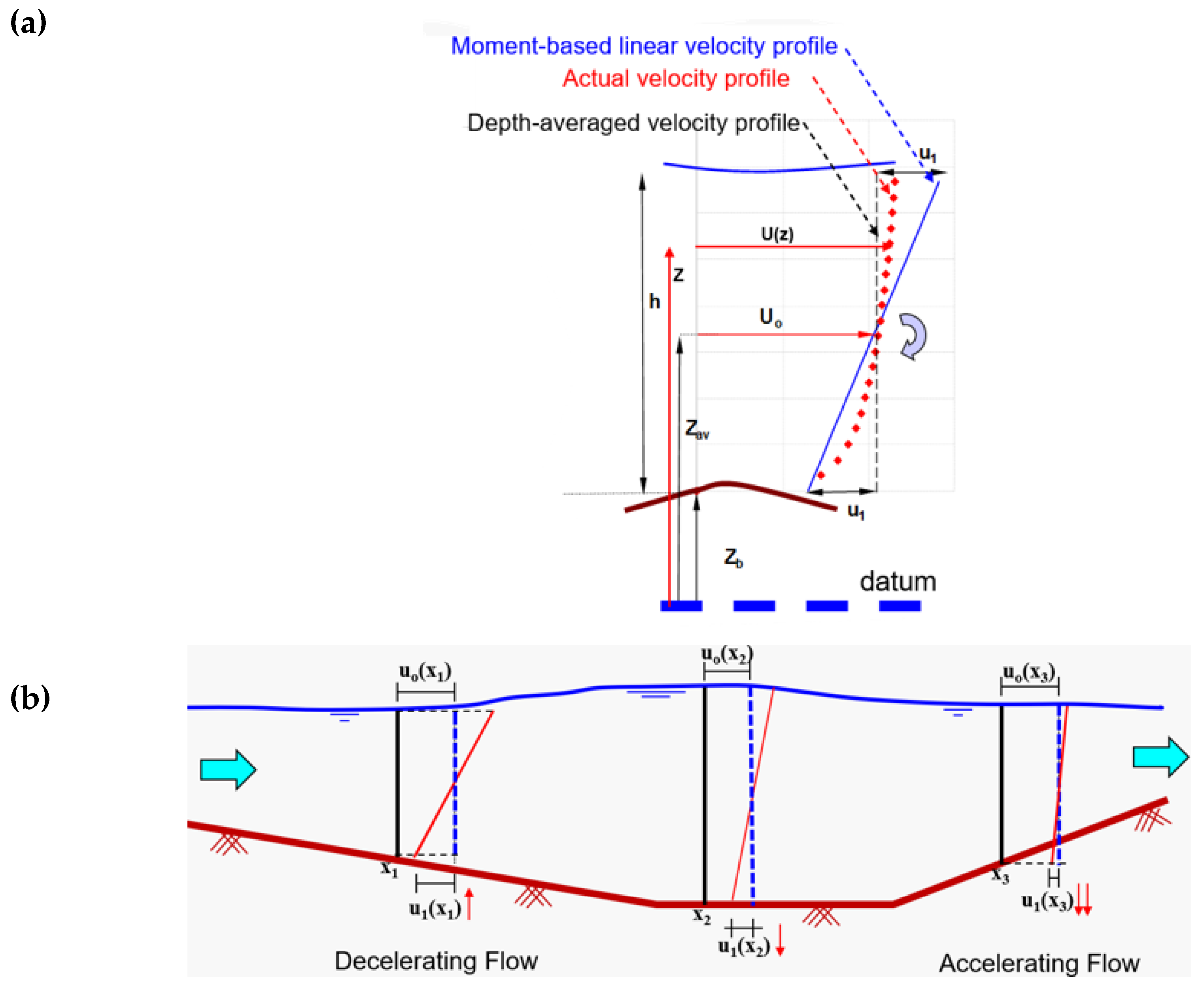
2.1. Moment of Momentum Concept
2.2. Selected Lab Experiments from the Literature
Criteria of Selection
2.3. Main Assumptions
3. Analysis Using an Empirical Approach
3.1. Selection of Velocity and Length Scales
- Mean Bed Level Up Crossings: Defined as the distance between two consecutive crossings of the mean bed level when ascending;
- Mean Bed Level Down Crossings: Signifying the distance between two successive crossings of the mean bed level when descending;
- Crest-to-Crest: Describing the distance between two consecutive crests;
- Trough-to-Trough: Denoting the distance between two successive troughs.
3.2. Dimensional Analysis
3.3. Velocity Functions and Flow/Boundary Conditions
3.3.1. Velocity Distribution Functions
3.3.2. Flow and Boundary Conditions
4. Results and Discussion
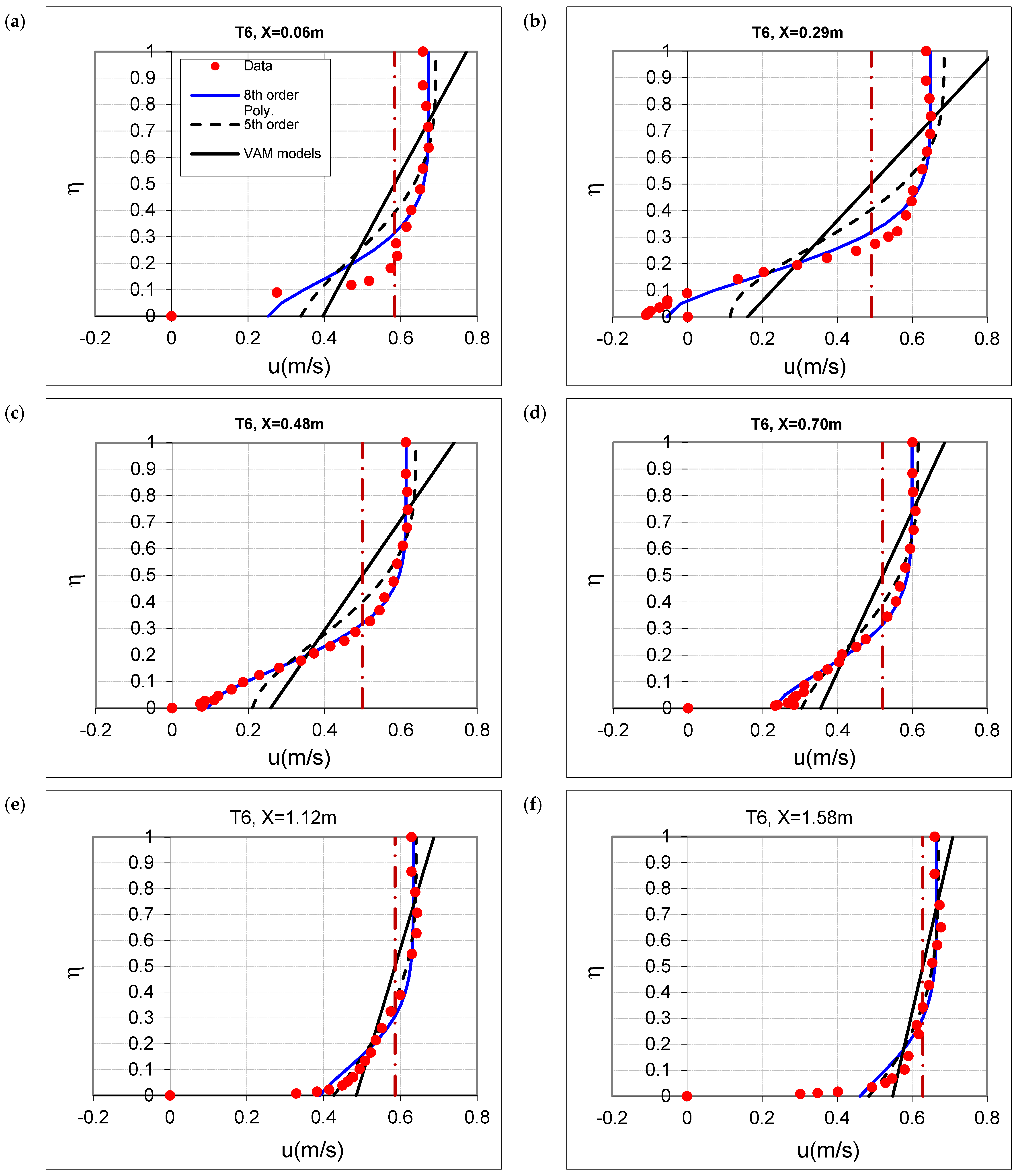
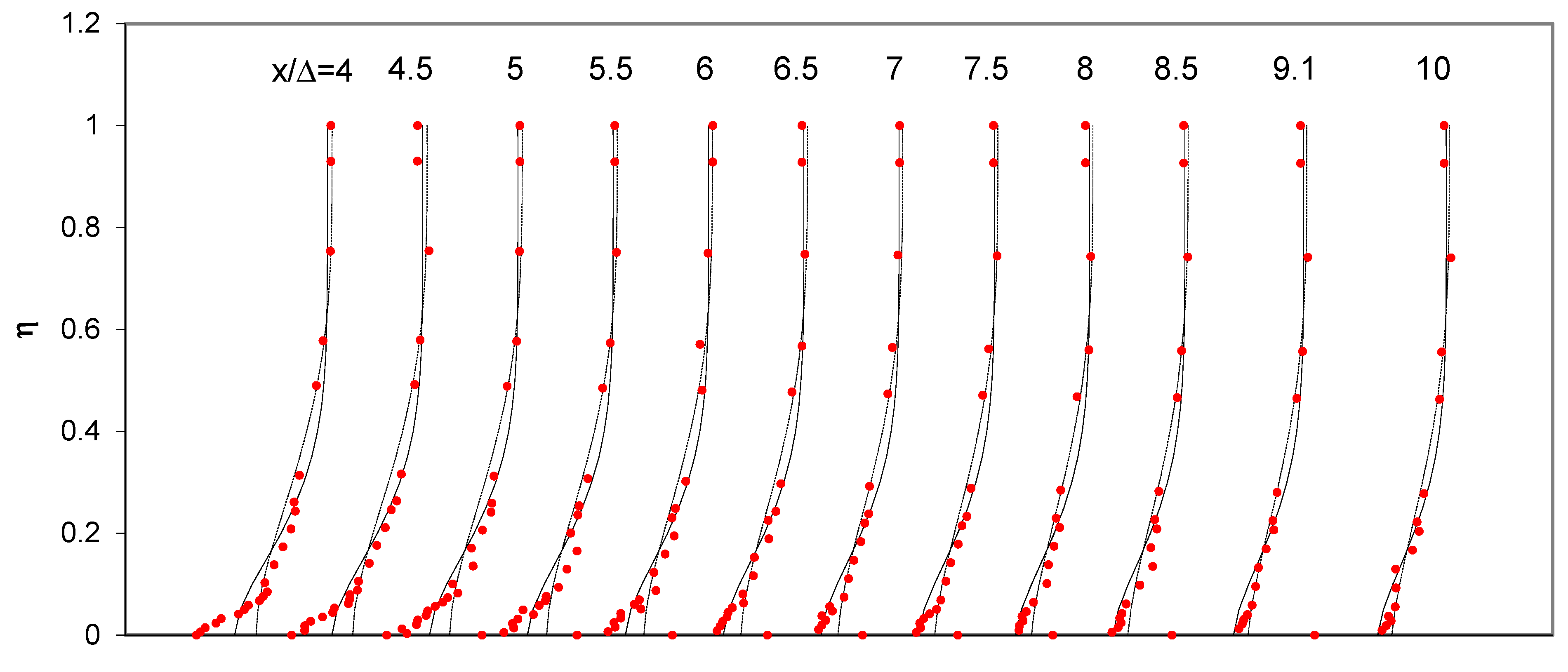
4.1. Verification of Flow over Bedforms
- The optimal constants for the log law vary based on the bedform’s location;
- As expected, the log law cannot accurately predict reverse flow and exhibits significant discrepancies within separation zones;
- A reasonable match with measurements near the crest can be achieved by optimizing the constants;
- Currently, no known formula exists for predicting the values of and over bedforms.
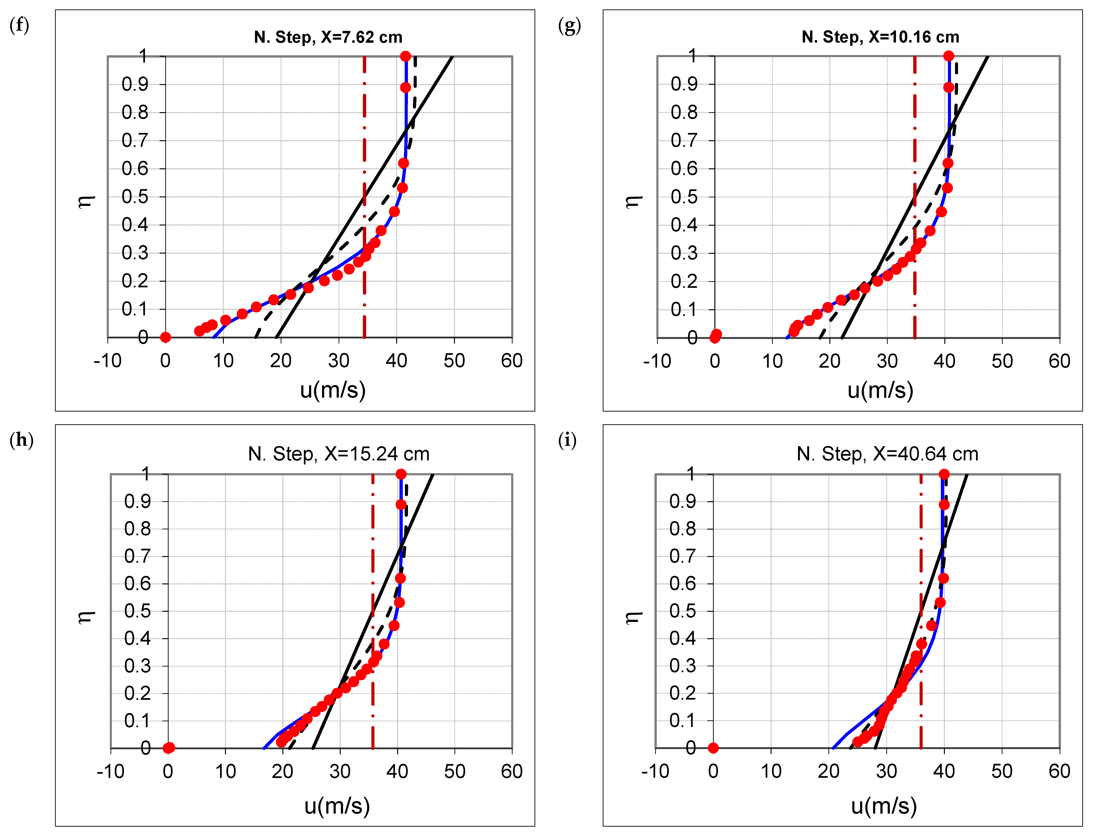
4.2. Evaluation in the Context of Negative Step Case
5. Conclusions
- The adoption of a slip boundary condition at the bed yielded improved agreement between the empirical velocity profiles and measurements, as opposed to the accuracy achieved by considering the more realistic no-velocity slip conditions;
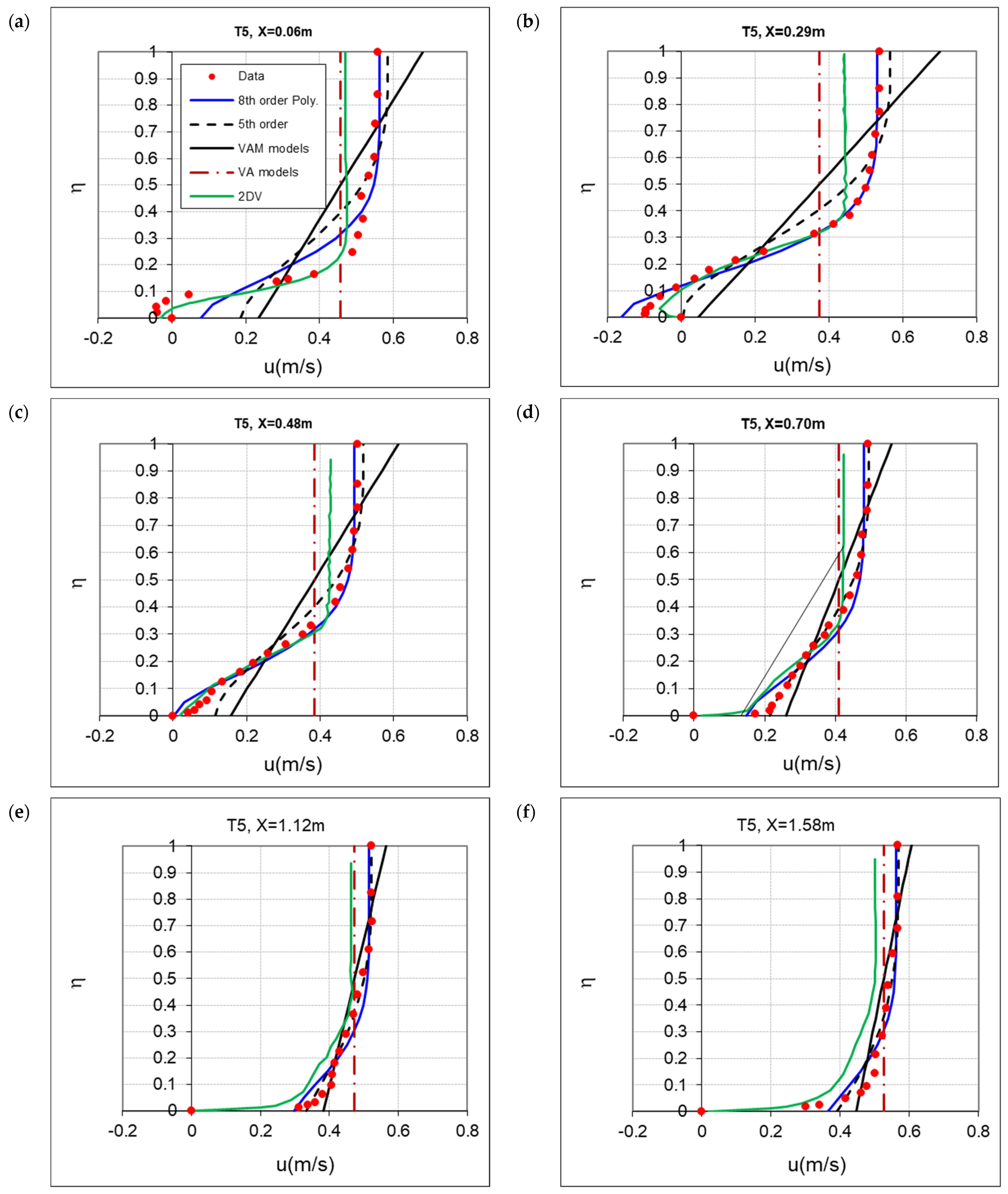
- While the linear profile exhibited limited agreement within the separation zone or near the point of reattachment where the velocity profile’s shape became notably non-uniform, it still represents an improvement over the uniform velocity assumption commonly employed in traditional depth-averaged flow models. As the downstream crest is approached, the acceleration of flow suggests better alignment with the linear profile;
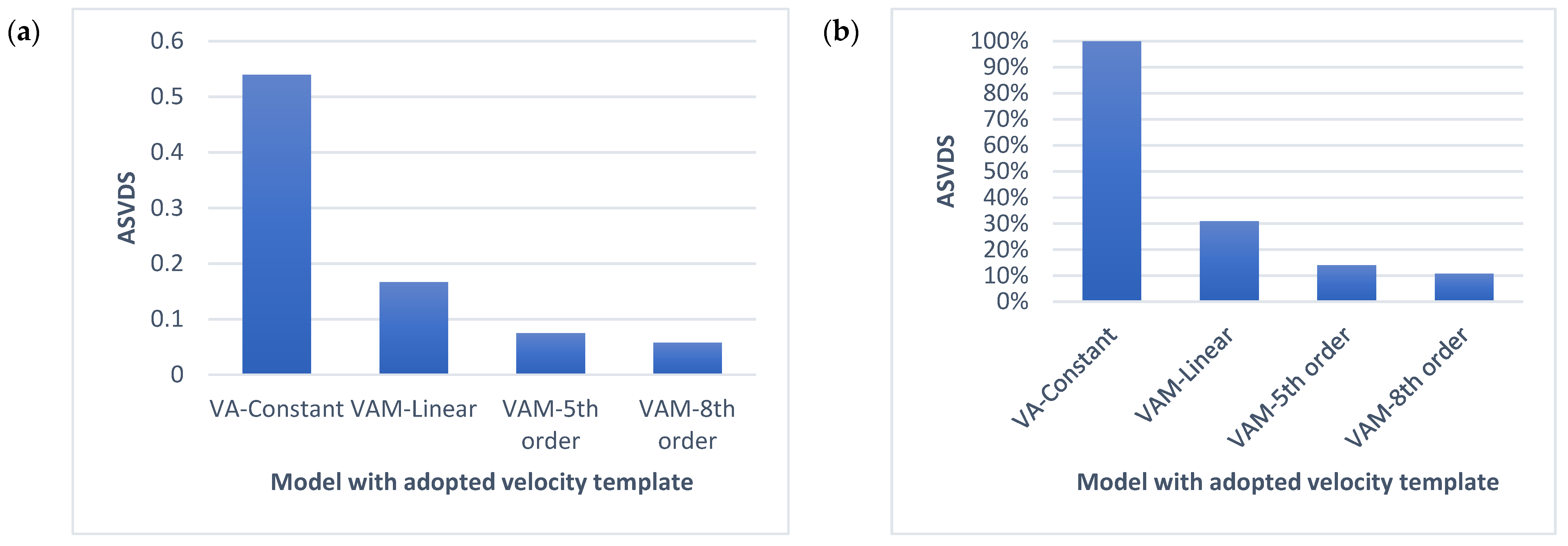
- Our findings reveal that linear velocity used in (VAM) models generally exhibits approximately 70% less velocity mismatch compared to the constant Vertically-Averaged (VA) models. Furthermore, the fifth-order and eighth-order velocity profiles demonstrate substantial improvements, with reductions in velocity mismatch of approximately 86% and 90%, respectively, compared to the VA models;
- The eighth-order polynomial profile generally yielded superior results within the eddy zone and proximity to the point of reattachment. Conversely, the fifth-order profile demonstrated better alignment downstream of the point of reattachment, particularly as the flow accelerated toward the crest.
- This novel approach was also successfully applied to the problem of airflow over a negative step within a wind tunnel, yielding satisfactory agreement with measured velocity data.
6. Limitations and Outlook
- The study in hand focuses on low-stage bedforms related to sand-bedded rivers and channels. Future work is required to assess the proposed approach for gravel-bedded bedforms;
- The analyses conducted in this study were centered on bedforms within the low-flow regime, specifically ripples and dunes, characterized by a low Froude number (Fn2 << 1). As a result, this study’s conclusions cannot be readily extrapolated to encompass high-flow regime scenarios involving antidunes and other bedform configurations. Exploring the behavior of high-flow regime bedforms presents a promising avenue for future research endeavors;
- Another notable limitation pertains to the assumption of one-dimensional (1D) bedforms with a uniform bed width. To expand the applicability of the analyses, future work could focus on extending the methodology to encompass two-dimensional (2D) bedforms, which presents a distinct set of challenges and considerations;
- Furthermore, this study primarily delved into fully developed turbulent flow over a non-erodible train of bedforms. Temporal aspects concerning the evolution of bedforms were excluded from the scope of this investigation, warranting potential exploration in forthcoming studies.
Funding
Institutional Review Board Statement
Informed Consent Statement
Data Availability Statement
Acknowledgments
Conflicts of Interest
Abbreviations
| a0-a5 | coefficients of 5th-order equations (refer to Equations (A1)–(A9)) |
| b0-b8 | coefficients of 8th-order equations (refer to Equations (A10)–(A19)) |
| b | channel/flume bed width |
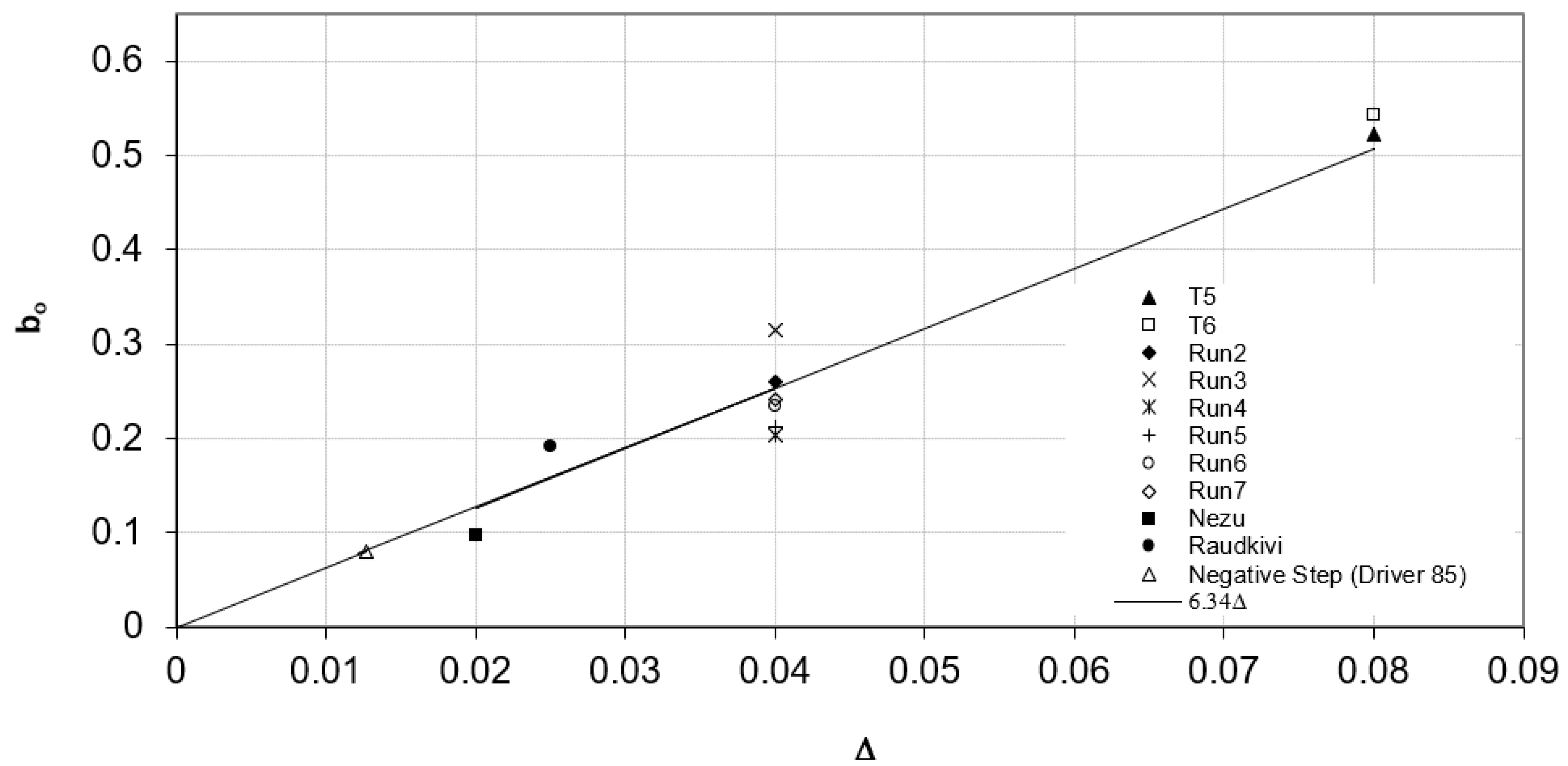
| bo | length scale (refer to Figure 5) |
| c | first constant in regression Equation (1) |
| C* | dimensionless Chezy coefficient |
| C2 | moment-based dimensionless Chezy coefficient (refer to Equation (12)) |
| d | second constant in regression Equation (1) |
| Fn | dimensionless Froude number |
| FCM | fully computational model |
| Ft | eddy viscosity coefficient |
| g | acceleration of gravity |
| h | local water depth at distance x |
| Kr | dimensionless calibration coefficient with a value ranging from about 1.45 to 2.7 |
| k | turbulent kinetic energy per unit mass |
| LDA | Laser Doppler Anemometry |
| PIV | Particle Image Velocimetry |
| q | specific discharge per unit width [m2/s] |
| q* | dimensionless variable (refer to Equation (12)) |
| qr | Near-bed velocity scale (refer to Equation (A8)) |
| SM | simplified model |
| u | Longitudinal velocity at a given station and elevation point |
| uo | longitudinal depth-averaged velocity at location x |
| u1 | Moment-based integral velocity scale along the flow x direction (refer to Figure 1) |
| u1o | value of u1 at the crest (refer to Figure 1) |
| u1log | moment velocity scale in the case of logarithmic velocity profile |
| u1* | normalized u1 value (Equation (2)) |
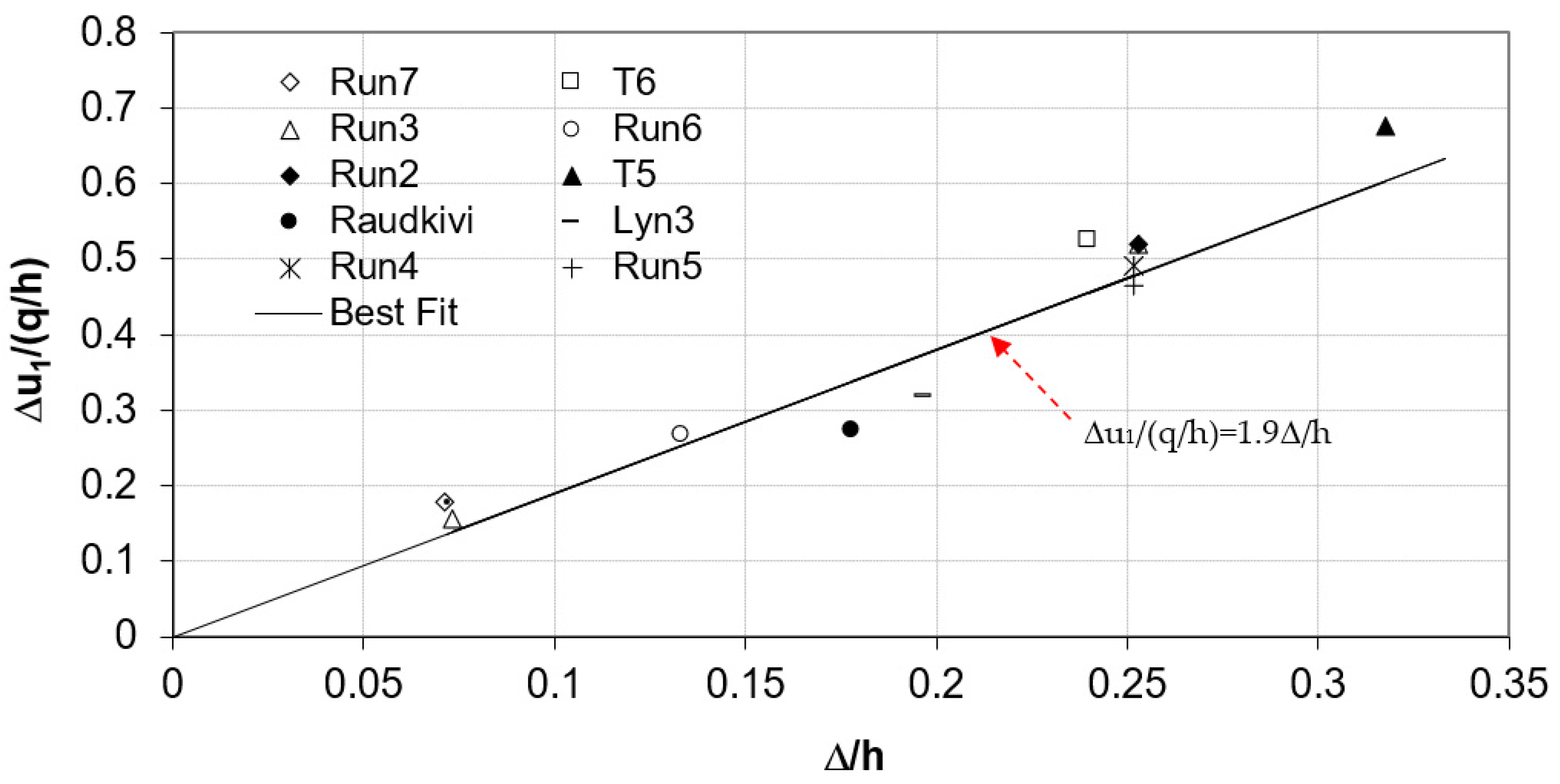
| Δu1 | the maximum net increase in the moment integral velocity |
| x | horizontal coordinate in the flow direction |
| z | vertical distance from a given arbitrary horizontal datum up to an arbitrary point (refer to Figure 1) |
| zav | vertical distance from a given arbitrary horizontal datum up to the mid-water depth |
| zb | local bed level |
| MofM | moment of momentum (refer to Figure 1) |
| VAM | Vertically Averaged and Moment model |
| Δ | bedform height |
| λ | bedform wavelength |
| ν | water kinematic viscosity coefficient |
| νt | eddy viscosity coefficient |
| h | Normalized water depth (refer to Equation (6)) |
Appendix A. Coefficients of Velocity Profiles
Appendix A.1. Coefficients of the 5th-Order Distribution
Appendix A.2. Coefficients of the 8th Order Distribution
References
- Keulegan, G.H. Laws of Turbulent Flow in Open Channels. J. Res. Natl. Inst. Stand. Technol. 1938, 121, 707–741. [Google Scholar] [CrossRef]
- Nezu, I.; Rodi, W. Open-channel flow measurements with a Laser Doppler Anemometer. J. Hydraul. Eng. ASCE 1986, 112, 335–355. [Google Scholar] [CrossRef]
- Coleman, N.L. Velocity profiles with suspended sediment. J. Hydraulic Res. 1981, 19, 211–229. [Google Scholar] [CrossRef]
- Guo, J.; Julien, P.Y. Application of modified log-wake law in open-channels. In Proceedings of the World Environmental and Water Resource Congress. Examining the Confluence of Environmental and Water Concerns, Omaha, Nebraska, 21–25 May 2006; pp. 1–9. [Google Scholar]
- Guo, J. Modified log-wake-law for smooth rectangular open channel flow. J. Hydraul. Eng. 2014, 52, 121–128. [Google Scholar] [CrossRef]
- Graf, W.H. Hydraulics of Sediment Transport; McGraw-Hill Inc.: New York, NY, USA, 1971; p. 513. [Google Scholar]
- Nakagawa, H.; Nezu, I. Experimental Investigation on Turbulent Structure of Backward-Facing Step Flow in an Open Channel. J. Hydraul. Res. 1987, 25, 67–88. [Google Scholar] [CrossRef]
- Engel, P. Length of flow separation over dunes. J. Hydraul. Eng. 1981, 107, 1133–1143. [Google Scholar] [CrossRef]
- Nelson, J.M.; McLean, S.R.; Wolfe, S.R. Mean flow and turbulence fields over two-dimensional bed forms. Water Resour. Res. 1993, 29, 3935–3953. [Google Scholar] [CrossRef]
- Smith, J.D.; McLean, S.R. Spatially Averaged Flow over a Wavy Surface. J. Geophys. Res. 1977, 82, 1735–1746. [Google Scholar] [CrossRef]
- McLean, S.R.; Smith, J.D. AModel for Flow over Two-Dimensional Bed Forms. J. Hydraul. Eng. 1986, 112, 300–317. [Google Scholar] [CrossRef]
- Haque, M.I.; Mahmood, K. Analytical determination of form friction factor. J. Hydraul. Eng. ASCE 1983, 109, 590–610. [Google Scholar] [CrossRef]
- Yoon, J.Y.; Patel, V.C. Numerical Model of Turbulent Flow Over Sand Dune. J. Hydraul. Eng. ASCE 1996, 122, 10–18. [Google Scholar] [CrossRef]
- Mendoza, C. Wen Shen H Investigation of Turbulent Flow over Dunes. J. Hydraul. Eng. ASCE 1990, 116, 459–477. [Google Scholar] [CrossRef]
- Johns, B.; Soulsby, R.L.; Xing, J. AComparison of Numerical Experiments of Free Surface Flow over Topography with Flume and Field Observations. J. Hydraul. Res. 1993, 31, 215–228. [Google Scholar] [CrossRef]
- Omidyeganeh, M.; Piomelli, U. Large-eddy simulation of three-dimensional dunes in a steady, unidirectional flow. Part 1. Turbulence statistics. J. Fluid Mech. 2013, 721, 454–483. [Google Scholar] [CrossRef]
- Keylock, C.J.; Chang, K.S.; Constantinescu, G.S. Large eddy simulation of the velocity-intermittency structure for flow over a field of symmetric dunes. J. Fluid Mech. 2016, 805, 656–685. [Google Scholar] [CrossRef]
- Chalmoukis, I.A.; Dimas, A.A.; Grigoriadis, D.G. Large-eddy simulation of turbulent oscillatory flow over three-dimensional transient vortex ripple geometries in quasi-equilibrium. J. Geophys. Res. Earth. Surf. 2020, 125, e2019JF005451. [Google Scholar] [CrossRef]
- D’Alessandro, G. Large-Eddy Simulation of the Flow over a Realistic Riverine Geometry. Ph.D. Thesis, Queen’s University, Kingston, ON, Canada, June 2023. [Google Scholar]
- Zhang, E.; Wang, Z.; Wu, W.; Wang, X.; Liu, Q. Secondary flow and streamwise vortices in three-dimensional staggered wavy-wall turbulence. Flow 2023, 3, E19. [Google Scholar] [CrossRef]
- Bhaganagar, K.; Hsu, T.J. Direct numerical simulations of flow over two-dimensional and three-dimensional ripples and implication to sediment transport: Steady flow. Coast. Eng. J. 2009, 56, 320–331. [Google Scholar] [CrossRef]
- Zgheib, N.; Fedele, J.J.; Hoyal, D.C.; Perillo, M.M.; Balachandar, S. Direct numerical simulation of transverse ripples: 1. Pattern initiation and bedform interactions. J. Geophys. Res. Earth. Surf. 2018, 123, 448–477. [Google Scholar] [CrossRef]
- Steffler, P.M.; Yee-Chung, J. Depth Averaged and Moment Equations for Moderately Shallow Free Surface Flow. J. Hydraul. Res. 1993, 31, 5–17. [Google Scholar] [CrossRef]
- Elgamal, M.H.; Steffler, P.M. A Bed Stress Model for Non-Uniform Open Channel Flow. In Proceedings of the 15th Hydrotechnical conference, CSCE, Victoria, BC, Canada, 30 May–2 June 2001. [Google Scholar]
- Ghamry, H.K.; Steffler, P.M. Two-dimensional depth-averaged modeling of flow in curved open channels. J. Hydraul. Eng. 2005, 43, 44–55. [Google Scholar] [CrossRef]
- Cantero-Chinchilla, F.N.; Bergillos, R.J.; Gamero, P.; Castro-Orgaz, O.; Cea, L.; Hager, W.H. Vertically averaged and moment equations for dam-break wave modeling: Shallow water hypotheses. Water 2020, 12, 3232. [Google Scholar] [CrossRef]
- Elgamal, M. A Moment-Based Chezy Formula for Bed Shear Stress in Varied Flow. Water 2021, 13, 1254. [Google Scholar] [CrossRef]
- Elgamal, M. A moment-based depth-averaged K-ε model for predicting the true turbulence intensity over bedforms. Water 2022, 14, 2196. [Google Scholar] [CrossRef]
- Van Mierlo, M.C.; De Ruiter, J.C. Turbulence measurements above artificial dunes. In Report on Measurements; Report Q789; Deltares (WL): Delft, The Netherlands, 1988; 1 and 2, Q789. [Google Scholar]
- Raudkivi, A.J. Study of sediment ripple formation. ASCE J. Hydraul. Div. 1963, 89, 15–33. [Google Scholar] [CrossRef]
- Raudkivi, A.J. Bed forms in alluvial channels. J. Fluid Mech. 1966, 26, 507–514. [Google Scholar] [CrossRef]
- Nezu, I. Free-surface flow structure of space-time correlation of coherent vortices generated behind dune bed. In Proceedings of the 6th Int. Symp. On Flow Modeling and Turbulence Measurements, Tallahasee, FL, USA, 8–10 September 1996; pp. 695–702. [Google Scholar]
- McLean, S.R.; Nelson, J.M.; Wolfe, S.R. Turbulence structure over two-dimensional bed forms: Implications for sediment transport. J. Geophysical Res. 1999, 99, 12729–12747. [Google Scholar] [CrossRef]
- McLean, S.R.; Wolfe, S.R.; Nelson, J.M. Predicting boundary shear stress and sediment transport over bed forms. J. Hydraul. Eng. 1999, 125, 725–736. [Google Scholar] [CrossRef]
- Van der Mark, C.F.; Blom, A. A New and Widely Applicable Bedform Tracking Tool; University of Twente: Enschede, The Netherlands; p. 2007.
- Engelund, F. Instability of Erodible Beds. J. Fluid Mech. 1970, 42, 225–244. [Google Scholar] [CrossRef]
- Huai, W.; Wang, W.; Zeng, Y. Two-layer model for open channel flow with submerged flexible vegetation. J. Hydraul. Eng. 2013, 51, 708–718. [Google Scholar] [CrossRef]
- Ahn, J.; Lee, J.; Park, S.W. Optimal Strategy to Tackle a 2D Numerical Analysis of Non-Uniform Flow over Artificial Dune Regions: A Comparison with Bibliography Experimental Results. Water 2020, 12, 2331. [Google Scholar] [CrossRef]
- Nelson, J.M.; Smith, J.D. Mechanics of Flow over Ripples and Dunes. J. Geophys. Res. 1989, 94, 8146–8162. [Google Scholar] [CrossRef]
- Schreider, M.I.; Amsler, M.L. Bedforms Steepness in Alluvial Streams. J. Hydraul. Res. 1992, 30, 725–743. [Google Scholar] [CrossRef]
- Driver, D.M.; Seegmiller, H.L. Feature of a Reattaching Turbulent Shear Layer in Divergent Channel Flow. AIAA J. 1985, 23, 163–171. [Google Scholar] [CrossRef]


| T5 (1) | T6 (1) | Raudkivi (2) | Nezu (3) | RUN2 (4) | RUN3 (4) | RUN4 (4) | RUN5 (4) | RUN6 (4) | RUN7 (4) | |
|---|---|---|---|---|---|---|---|---|---|---|
| h (m) | 0.252 | 0.334 | 0.135 | 0.08 | 0.158 | 0.546 | 0.159 | 0.159 | 0.3 | 0.56 |
| q (m2/s) | 0.1 | 0.18 | 0.035 | 0.023 | 0.06 | 0.153 | 0.058 | 0.032 | 0.16 | 0.133 |
| λ (m) | 1.6 | 1.6 | 0.386 | 0.42 | 0.807 | 0.807 | 0.408 | 0.408 | 0.408 | 0.408 |
| Δ (m) | 0.08 | 0.08 | 0.0225 | 0.02 | 0.04 | 0.04 | 0.04 | 0.04 | 0.04 | 0.04 |
| Rn | 73,370 | 117,338 | 8000 | 16,429 | 44,408 | 69,127 | 42,857 | 23,645 | 96,000 | 59,257 |
| ks (mm) | 2.4 | 2.4 | 0.6 | 0.1 | 0.75 | 0.75 | 0.75 | 0.75 | 0.75 | 0.75 |
| C* | 17.02 | 17.53 | 15.34 | 19.15 | 18.33 | 19.99 | 18.32 | 17.99 | 19.51 | 19.92 |
| u* (m/s) | 0.0222 | 0.0284 | 0.0169 | 0.0150 | 0.0207 | 0.0140 | 0.0199 | 0.0112 | 0.0273 | 0.0119 |
| λ/Δ | 20 | 20 | 15.4 | 21 | 20.2 | 20.2 | 10.2 | 10.2 | 10.2 | 10.2 |
| Δ/h | 0.3 | 0.23 | 0.19 | 0.25 | 0.25 | 0.07 | 0.25 | 0.25 | 0.13 | 0.07 |
| Fn | 0.24 | 0.27 | 0.23 | 0.32 | 0.31 | 0.12 | 0.29 | 0.16 | 0.31 | 0.1 |
| b (m) | 1.5 | 1.5 | 0.08 | 0.4 | 0.9 | 0.9 | 0.9 | 0.9 | 0.9 | 0.9 |
| Flume Length (m) | >53 | >53 | 2.45 | 10 | 8 | 8 | 8 | 8 | 8 | 8 |
| Velocity Device | LDA | LDA | Pitot Tube | LDA | LDA | LDA | LDA | LDA | LDA | LDA |
Disclaimer/Publisher’s Note: The statements, opinions and data contained in all publications are solely those of the individual author(s) and contributor(s) and not of MDPI and/or the editor(s). MDPI and/or the editor(s) disclaim responsibility for any injury to people or property resulting from any ideas, methods, instructions or products referred to in the content. |
© 2023 by the author. Licensee MDPI, Basel, Switzerland. This article is an open access article distributed under the terms and conditions of the Creative Commons Attribution (CC BY) license (https://creativecommons.org/licenses/by/4.0/).
Share and Cite
Elgamal, M. Mapping Mean Velocity Field over Bed Forms Using Simplified Empirical-Moment Concept Approach. Water 2023, 15, 3351. https://doi.org/10.3390/w15193351
Elgamal M. Mapping Mean Velocity Field over Bed Forms Using Simplified Empirical-Moment Concept Approach. Water. 2023; 15(19):3351. https://doi.org/10.3390/w15193351
Chicago/Turabian StyleElgamal, Mohamed. 2023. "Mapping Mean Velocity Field over Bed Forms Using Simplified Empirical-Moment Concept Approach" Water 15, no. 19: 3351. https://doi.org/10.3390/w15193351
APA StyleElgamal, M. (2023). Mapping Mean Velocity Field over Bed Forms Using Simplified Empirical-Moment Concept Approach. Water, 15(19), 3351. https://doi.org/10.3390/w15193351