Abstract
The occurrence of bridge collapse is frequently attributed to the prevalent erosion in the vicinity of bridge abutments. Accurate determination of the maximum scour depth in the vicinity of bridge abutments is imperative to ensure a secure and reliable bridge design. The phenomenon of local scour at bridge abutments can exhibit significant variations when compared to open-flow conditions, primarily due to the additional obstacle posed by the presence of ice cover. Research has demonstrated that the erosion of bridge abutments is more pronounced in the presence of ice. The vertical velocity distribution has a direct impact on both the bed shear stress and the resulting scour geometry in ice-covered conditions. This study aims to analyze the effects of flow through open channels and covered flow conditions on the local scour process around semi-circular and square bridge abutments using FLOW-3D V 11.2 software. The utilization of the volume of fluid (VOF) approach is employed for monitoring the free surface, while the Reynolds averaged Navier-Stokes (RANS) equations and the RNG k turbulence model are employed for simulating the flow field in the vicinity of bridge abutments. The sediment transport equations formulated by Meyer-Peter and Müller were employed for the purpose of simulating the movement of sediment particles. The numerical simulation results are compared with the experimental results. The result shows that the presence of ice cover and its roughness can increase the maximum scour depth both in numerical and experimental studies. The results also indicate that the maximum scour depth is located at the upstream section of the bridge abutments. These findings demonstrate the ability of the numerical model to predict the occurrence of local scour in the vicinity of bridge abutments under conditions of ice presence.
1. Introduction
Local scour refers to the erosive process that occurs as a result of alterations in the immediate flow pattern caused by the introduction of obstacles within the flow [1]. The phenomenon of local scour, which manifests in the vicinity of bridge and offshore platform foundations, poses a threat to the stability of these foundations and has the potential to result in the collapse of the primary structures. As the scour depths in the vicinity of foundations become larger, there is a corresponding decrease in the insertion depths of bridge abutments and piers. This decrease in insertion depths is directly linked to the stability of bridge foundations. The occurrence of erosion in the vicinity of a bridge’s substructure is a widely observed factor contributing to the failure of bridges, leading to substantial economic repercussions on a global scale. Over the course of the last three decades, the United States has experienced the collapse of more than a thousand bridges, with pier scour being identified as the cause in sixty percent of these instances [2,3]. A study conducted by Foti and Sabia (2010) has revealed that over 26,000 bridges in the United States have been designated as scour critical [4].
In 1994, a significant number of railway spans, specifically 49, were adversely affected by localized erosion [5]. The rail traffic in China was disrupted for a duration of 2319 h due to a derailment incident [4]. Several scholarly investigations have been conducted on the phenomenon of local scour in the vicinity of bridge abutments within open channels. These studies include the works of Froehlich (1989), Melville (1999), Coleman (2005), and Dey and Sarkar (2006) [6,7,8,9].
In regions such as Canada and other northern areas characterized by cold climates, it is not uncommon for ice cover to endure for a duration of up to six months. The intricate interplay of hydrodynamic, mechanical, and thermal phenomena significantly contributes to the intricate nature of local scour formation in the vicinity of bridge foundations during periods of ice cover [10]. The occurrence of a scour hole is commonly accompanied by the presence of three vortex systems in the vicinity of the abutment. Based on the research conducted by Kwan and Melville (1994), it can be inferred that the scour hole is primarily affected by a significant primary vortex and the subsequent downward flow [11]. The primary vortex undergoes downstream expansion beyond the abutment and subsequently dissipates its distinct characteristics over a certain distance. At the location where the abutment meets the downstream area, there is an increase in flow velocity, leading to the creation of localized swirling patterns referred to as wake vortices. The creation of wake vortices is achieved by isolating the flow between the upstream and downstream abutment boundaries [11]. According to the study conducted by Kwan and Melville (1994), it was found that alterations in the depth of the approach flow have minimal impact on both the flow pattern and the maximum downflow in open channel flow conditions [11]. Research has shown that the presence of a stable ice cover in natural waterways leads to a significant increase in the wet perimeter and a migration of the maximal velocity towards the channel bed. Consequently, this results in an elevation of the bed shear stress. The study conducted by Zabilansky and White (2005) examined the influence of ice cover on the occurrence of local scour in rivers with restricted flow. According to their study, it was found that when ice cover is present, an increase in discharge and the presence of ice leading to a pressurized flow condition can result in the migration of the flow’s maximum velocity closer to the bed [12]. Wu et al. (2015) examined the impact of varying levels of relative substrate coarseness, flow shallowness, and pier height. The Froude number’s influence on the phenomenon of local scour around a bridge pier was examined in a study, which found that the depth of scour is greater when the pier is covered compared to when it is exposed to open channel flow conditions [12]. Wu et al. (2015) further examined the morphology of scouring near bridge abutments in the presence of ice. The researchers observed that sediment sorting under ice cover was more noticeable at different points surrounding the abutment [13]. Insufficient scholarly investigation has been undertaken regarding the occurrence of localized erosion in the vicinity of bridge abutments during periods of ice cover. Namaee et al. (2021) conducted experiments and employed 3D numerical models to elucidate the disparities in scour phenomena between two neighboring circular piers, considering the presence or absence of ice [14].
The utilization of numerical analysis has witnessed a growing prevalence in the field of hydrodynamics. CFD models possess the advantages of being both cost-effective and time efficient. Additionally, they are not influenced by scale effects and can be utilized across various geometries and hydraulic conditions pertaining to a specific hydraulic issue [15]. Richardson and Panchang (1998) employed a comprehensive three-dimensional hydrodynamic model to simulate the flow pattern occurring within a scour hole situated at the base of a cylindrical bridge substructure [16]. Vasquez and Walsh (2009) employed the FLOW-3D software to conduct a simulation of the early stages of scour development in a structurally intricate pier consisting of ten sizable cylindrical pile caps [17]. In a study conducted by Kim et al. (2014), a Large-eddy simulation (LES) was employed to model the turbulent flow around cylinders. This simulation aimed to investigate the impact of the transverse and longitudinal spacing distance between cylinders on various aspects, including scour evolution, bed topography, flow structure, and maximum scour depth [18].
There is little research in the field that looks at how numerical simulations and real-world experiments differ when it comes to the complicated phenomenon of local scour near bridge abutments under ice conditions. To fill in this gap, the current study uses FLOW-3D software, which is a computational fluid dynamics tool, to study the complicated process of local erosion that happens near bridge abutments with the presence of ice cover. This study aims to investigate the interaction among the flow, the thickness of the ice, and the changes in the shape of scour holes. By doing a systematic study, this research hopes to shed light on the complicated relationship between how turbulent energy is spread out and how the shape of the scour hole changes as a result. This study looks at both times when the bridge support is covered in ice and open channel conditions. By looking at these complicated parts under different situations, this study hopes to learn more about how the different parts of the under-ice scour phenomenon work together. Also, using advanced numerical simulations is a new way to understand this complicated phenomenon. These simulations could provide more nuanced and detailed information than traditional experimental methods. In short, the current study is an important step toward filling in the gaps about how numerical modeling and real-world experiments compare in the case of local scour around bridge abutments caused by ice cover. This study has the potential to enhance our understanding of the under-ice scour process and its underlying causes. It achieves this by examining the distribution of turbulent energy and alterations in water morphology.
2. Experiment Setup
The present study employed a channel of considerable dimensions, measuring 2 m in width, 1.3 m in depth, and 38.2 m in length. Figure 1 shows the experimental setup. The flow rate of the channel was regulated through the utilization of an inlet valve. To mitigate the turbulence of the incoming flow, flow dissipators were implemented upstream of the channel. Two sandboxes with similar dimensions were utilized to accommodate three distinct types of non-uniform sediments. The sediments were placed within the sandboxes, with a depth of 0.30 m. The three sediment mixtures examined in this study exhibited non-uniformity, as indicated by their respective D50 values of 0.58 mm, 0.50 mm, and 0.47 mm. Additionally, the geometric standard deviations (σg) associated with these mixtures were found to be 2.61, 2.53, and 1.89, respectively. Based on the findings of Dey and Barbhuiya (2004), it can be inferred that the sediments under investigation exhibit non-uniform characteristics, as indicated by the values of σg exceeding 1.4 [19]. This study aimed to compare the shape factor of abutments, as defined by Melville (1992), by evaluating semi-circular and square-shaped abutments [20]. The abutments were constructed using plexiglass material, and they were equipped with clearly visible measuring lines on their outer surfaces. This allowed for the convenient assessment of scour depths at different positions (see Figure 2). In the case of the square abutment, four equidistant lines were delineated on the upstream surface. Conversely, for the semi-circular abutment, twelve lines were marked along the abutment, each having equal central angles of 15 degrees. To replicate the occurrence of ice on the surface of water, both smooth and uneven coverings were employed. The creation of uneven covers involved the attachment of 0.025m cubes, with a spacing of 0.03m, to the lower surface of smooth covers. The uneven surface utilized in the investigations is illustrated in Figure 3a. In front of the first sandbox, a 2D Flow Meter was installed to measure flow velocities and water depth (Figure 3b). A staff gauge was also installed in the middle of each sandbox to manually verify water depth. A 10 MHz SonTek Acoustic Doppler Velocimeter (ADV) was applied to measure the instantaneous velocity in the scour hole around the abutment at different locations and elevations. After all the velocity measurement was completed, the flume was drained completely, and the scour hole was measured. The operational state of the SonTek IQ velocity meter is illustrated in Figure 3b. The SonTek was placed upstream of the channel to measure approaching flow velocity and volumetric flow discharge. The velocity range in the first sandbox spanned from 0.16 to 0.26 m/s, whereas in the second sandbox, it ranged from 0.14 to 0.21 m/s. A tailboard was implemented at the terminal point of the channel in order to control and adjust the water depth. Based on the observations, it was determined that it took a total of 24 h for the scour depth to reach its maximum value in the vicinity of the abutments. Before each test, the flume is filled with water slowly, and after the required water depth is reached, Styrofoam is put on top of the water as a simulated ice cover. After the depth is reached, then the experiment is started. A total of 54 experiments were conducted. The characteristics of experiments related to square abutments are shown in Table 1. These experiments were carried out on semi-circular and square bridge abutments under open channels, and smooth and rough ice flow conditions. In order to measure scour depths, a caliper was used.
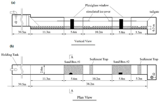
Figure 1.
The experimental setup is from two different perspectives: (a) a side view and (b) a top view.
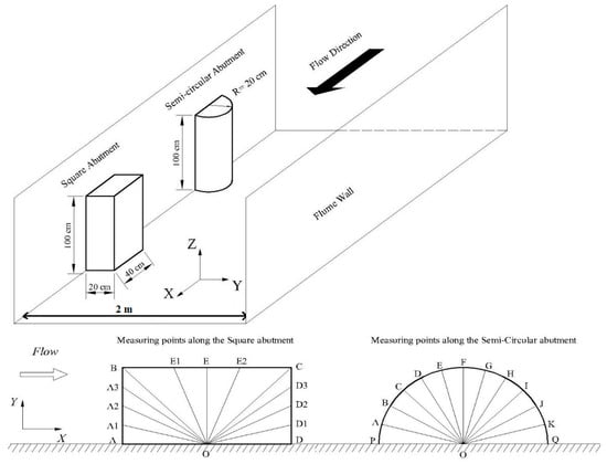
Figure 2.
The dimensions and measuring points are located adjacent to the abutments.
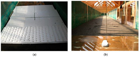
Figure 3.
(a) The surface of the cover exhibits irregularities in the form of cubes of varying heights and positions. (b) The SonTek IQ velocity meter is installed in a position upstream from the abutments.

Table 1.
Test condition and non-uniform sediment composition of each experiment for square abutment.
3. Numerical Model
In the current investigation, the widely utilized computational fluid dynamics (CFD) model FLOW-3D was utilized [21,22,23,24,25,26]. The volume of fluid (VOF) method is employed by FLOW-3D to accurately track the movement of the free water surface [27]. The Fractional Area/Volume Obstacle Representation (FAVOUR) method is employed in FLOW-3D to simulate intricate geometric regions, such as compacted sediment, within rectangular meshes [28]. The area fractions (Ai) are determined at each of the six faces by calculating the ratio of the specific open area to the total area within each mesh grid. Similarly, the volume fraction (VF) is determined by calculating the ratio of the fluid-accessible volume to the total volume of the grid. The artificial intelligence (AI) and virtual framework (VF) that are linked to the compacted sediments are regularly updated during each time increment to accurately represent the alterations in the geometry of the compacted sediments. The FAVOUR method is capable of accurately determining the geometry by utilizing a smaller number of mesh grids compared to the finite difference method (FDM), resulting in a notable reduction in computation time [29].
3.1. Governing Equations
The FLOW-3D software integrates multiple turbulence models, a sediment transport model, and an empirical bed erosion model. These models are used in conjunction with the Volume of Fluid (VOF) technique to accurately compute the free surface of the fluid without the need to solve for the air component [27]. The RANS equations, which are employed to describe the motion of incompressible viscous fluids around bridge abutments, are closed using the RNG k turbulence model. Equations (1)–(4) encompass the fundamental Reynolds-Averaged Navier-Stokes (RANS) equations and the continuity equation, which describe the behavior of Newtonian, incompressible fluid flow. These equations incorporate the variables. The equations presented encompass area fractions (Ai) and volume fractions (VF).
where
In the given context, the variables can be defined as follows: ui represents the velocity component in the i direction, Ai represents the fractional area in the i direction, VF represents the volume fraction of fluid in each grid, p represents the pressure, t represents time, gi represents the gravitational force in the i direction, ρ represents the mass density of the fluid, and fi represents the diffusion transport term. The strain rate tensor, denoted as Sij, represents the rate at which a material deforms. The wall shear stress, τb,i, refers to the force per unit area exerted on a surface parallel to a fluid flow. The kinematic viscosity, v, is a measure of a fluid’s resistance to flow. Lastly, the kinematic eddy viscosity, νT, represents the turbulent diffusion of momentum in a fluid.
3.2. Turbulent Model
FLOW-3D is capable of accommodating various turbulence models, including the one-equation model, two-equation models such as conventional k, RNG k-, and k- models, as well as Large Eddy Simulation (LES). The susceptibility of the sediment scour model to turbulence modeling is primarily attributed to the direct impact of the turbulence model on the computed viscosity within FLOW-3D. It is worth mentioning that viscosity plays a crucial role in the computation of local shear stress, which is employed in the determination of bed-load erosion and entrainment rates. The RNG k model is utilized to incorporate the impacts of smaller scales of motion in the simulation of sediment scour by renormalizing the Navier-Stokes equations [30]. The RNG model incorporates enhancements to the conventional k model that augment its effectiveness. The current study employs the RNG k turbulent model to simulate the localized erosion occurring in the vicinity of bridge foundations. The governing equations of the RNG k model incorporate the area and volume fractions, similar to how the continuity and momentum conservation equations are included [30].
3.3. Sediment Scour Model
The coupling of fluid flow and sediment scour models in Flow-3D is complete [29]. The analysis encompasses various mechanisms involved in the transportation of non-cohesive soil sediment, encompassing both suspended and bed-load transport, as well as processes such as entrainment and deposition. This software enables the simulation of a wide range of non-cohesive sediment species, each possessing distinct characteristics, including mass density, critical shear stress, particle size, angle of repose, and transport parameters. The model estimates the movement of sediment particles by forecasting their erosion, advection, and deposition. The sediment scour model incorporates four distinct sediment transport mechanisms that serve to delineate and characterize sediment transport processes. The initial process involved in sediment transport is known as entrainment. This phenomenon takes place when the critical shear stress falls below the bed shear stress, resulting in the elevation and subsequent suspension of sediment particles located at the uppermost layer of a densely packed bed. The second mechanism observed in sediment transport is known as suspended load transport, wherein sediment particles are transported by the fluid flow at a specific elevation above the consolidated substrate.
The third mechanism, known as deposition, is characterized by a decrease in the flow’s capacity to transport suspended sediments. This decrease is primarily influenced by the forces of gravity, buoyancy, and friction. Consequently, the suspended sediments are deposited in areas where the diminishing flow lacks the ability to continue their movement. The ultimate mechanism of sediment transport is bed-load transport, wherein granules are mobilized by fluid-induced shear stress and move by rolling, sliding, or hopping along the bed [31,32,33]. Hence, a sediment scour model can be employed to calculate the transport of suspended sediment, sediment settling caused by gravitational forces, sediment entrainment resulting from bed shearing and flow disturbances, and bed-load transport, wherein sediment particles roll, hop, or slide along a compacted sediment bed [34].
Deposition and Entrainment
Deposition refers to the phenomenon in which sediment particles, either due to their weight or during bed-load transport, settle out of suspension and come to rest on a compacted bed. The processes of grain settling and entrapment are often observed to occur simultaneously despite being opposite in nature [29]. Besides, Suspended sediments are carried along with the fluid flow by advection. In terms of bed-load transport, it refers to the process by which sediments are transported across a sediment bed surface through rolling, sliding, or bouncing movements. The volumetric transport rate of sediment per width of the bed in FLOW-3D is determined by three equations, which are the models proposed by Meyer-Peter and Müller (1948), Nielsen (1992), and Van Rijn (1984) [35,36,37]. The present study has used Meyer-Peter and Müller’s equation [35]. Note that Meyer-Peters formulation is generally used for high bed load conditions where sediment transport by saltation and rolling is dominant. The numerical results showed that the use of the Meyer-Peters formulation may be appropriate since the rate of sediment transport was high in the vicinity of bridge abutments.
3.4. Model Setup
A numerical simulation was conducted to investigate the phenomenon of local scour around square and semi-circular bridge abutments in a channel with a median grain size (d50) of 0.50 mm. In order to replicate the phenomenon of local scouring around bridge abutments in open channel environments, both smooth and irregular flow conditions with ice cover, a set of six numerical models was constructed. These numerical models were performed for open channel, smooth, and rough ice covers for semi-circular and rectangular abutments in a channel with a median grain size (d50) of 0.50 mm, which are discussed in more detail below. The intended length of the numerical simulation channel section was 5 m. The abutments of the bridge were positioned in the identical location as in the corresponding experiments. The computational domain’s length was adequate to guarantee the absence of any interference between the turbulent stream and the boundary downstream. The sediment substrate exhibited a depth of 0.30 m. The critical shields parameter was determined using the equation proposed by Soulsby and Whitehouse (1997) [34]. Soulsby and Whitehouse (1997) assume there is a maximum of 0.3 for the critical Shields parameter. Note that the Shields parameter, also known as the Shields criterion, is used in the field of sediment transport to predict when sediment particles will begin to move due to the force of flowing water or other fluids. The critical value of the Shields parameter depends on various factors, including the size and shape of the sediment particles, the properties of the fluid, and the geometry of the channel. The default value for the angle of repose, which denotes the maximum resting angle of the bed, was established at 32 degrees. To assess the potential extension of the current numerical models for simulating sediment transport around bridge abutments under ice-covered conditions, the corresponding parameters in the experiments were kept consistent in order to evaluate the applicability, validity, and precision.
3.4.1. Meshing
The computational domain’s length was found to be 5.6 m, which is similar to the length observed in the experimental study. Two separate geometry grids were created, each with different levels of resolution. Mesh convergence analysis helps researchers determine whether their simulation results are converging toward a stable solution as the mesh becomes finer. This is essential for ensuring that the results are not significantly influenced by the choice of mesh size. Mesh convergence analysis helps assess the effectiveness and accuracy of the numerical model by studying how the results change with varying levels of mesh refinement. In this study, simulations were then conducted to assess the impact of grid resolution. Both types of mesh grids cover the entire computational domain with a multi-block mesh that comprises three mesh blocks. Prior to grid optimization, the initial configuration of the mesh grid consisted of three mesh blocks, each with a uniform size of 20 mm throughout the entire domain. In contrast, the optimized second form of the mesh grid featured a finer grid size of 20 mm × 20 mm for the middle mesh block where the piers were positioned. The middle mesh block, which consisted of a finer grid mesh, spanned the section of the channel from 0.5 m to 4.5 m. To decrease computational time, coarser grid meshes with dimensions of 30 mm × 30 mm were employed for the initial mesh block spanning from 0.0 m to 0.5 m, as well as for the third mesh block ranging from 4.5 m to 5.0 m. The sensitivity analysis revealed that employing coarser grids for the first and third mesh blocks did not yield any significant modifications to the simulated bed scour. When the calculated maximum scour depth (MSD) prior to grid optimization exhibits a difference of less than 5% compared to the calculated maximum scour depth (MSD) after grid optimization, this disparity is considered to be inconsequential. The total number of grid cells is 1,072,963, with 35,376 allocated to the first mesh block in the upstream section, 1,000,000 allocated to the second mesh block in the intermediate section, and 37,587 allocated to the third mesh block in the downstream section (Table 2).
Table 2.
Characteristics of mesh used in this study.
3.4.2. Boundary Conditions
The boundary conditions for the numerical models are illustrated in Figure 4a,b. Figure 4a represents the conditions of an open channel, while Figure 4b represents the conditions of uneven ice-covered flow. In conjunction with the prescribed boundary conditions for the abutment surface and the ice cover surface, it is necessary to establish fixed boundaries for a total of six distinct meshes. The sidewall mesh boundaries were assigned as no-slip walls, the top boundary was designated as symmetry, the bottom boundary was set as no-slip wall, the inlet boundary on the left was prescribed with a specific velocity, and the outlet boundary on the right was defined as out-flow boundaries. In the scenario of smooth ice-covered flow, a non-floatable smooth ice cover was replicated in the physical model, maintaining the same water depth. Conversely, in the case of uneven ice-covered flow, the physical model included simulated 25 mm ice cubes in addition to the smooth ice cover. In this configuration, the fluid motion progresses horizontally from the left side to the right side, running parallel to the impermeable walls and confined within the space between the non-permeable floor and the sediment bed until it reaches the boundary where the out-flow occurs.
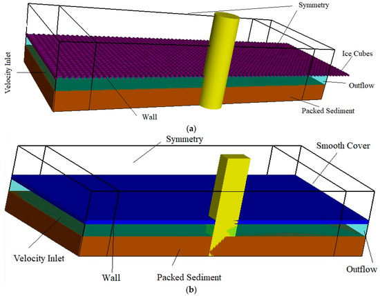
Figure 4.
(a) The simulation model and boundary conditions for the semi-circular bridge abutment under uneven ice-covered flow conditions. (b) The simulation model and boundary conditions for the square bridge abutment under smooth ice-covered flow conditions.
4. Results and Discussion
This section presents an analysis of the mechanisms involved in local scour around semi-circular and square bridge abutments under various conditions, including open channel flow, smooth ice cover, and irregular ice cover. The numerical results obtained from this analysis are then compared to experimental cases. The quantitative findings encompass the scour depth, morphological alterations, and deposition patterns in the proximity of the bridge abutments. Typically, irrespective of the presence of ice cover, the maximum depth of scour for both categories of abutments is observed on the upstream side, facing the incoming flow. The maximum scour depth for a semi-circular abutment occurs at an angle of 75 degrees with respect to the approaching flow (referred to as Point E in Figure 2). Conversely, for a square abutment, the highest scour depth is observed at the upstream corner, which is closer to the center of the channel (identified as Point B in Figure 2). The scour hole exhibited a consistent pattern irrespective of the presence of ice cover; however, the development of scour holes was more pronounced in the presence of ice cover, particularly in cases where the ice cover was asymmetrical.
4.1. Local Scour around Square Abutment under Open Channel Flow Condition
In a manner akin to the experimental setup, the numerical experiment was performed utilizing an inflow velocity of 0.21 m/s and a uniform water depth of 0.19 m. Simulations were conducted using sediment with a median grain size of 0.50 mm (D50 = 0.50 mm). Figure 5a illustrates the numerical representation of the local scour that has formed around the square bridge abutment after a duration of 600 s, during which the scour depth has reached a state of equilibrium. Note that the difference in the time it took to reach equilibrium between the simulation (600 s) and the actual experiment (24 h) could be due to several factors, such as simulations, boundary conditions, model accuracy, and initial conditions. Scale and simplification often involve simplifications and scaling down of the physical system. These simplifications can result in faster convergence to equilibrium. Real-world experiments are subject to a wide range of complex, uncontrolled variables that can slow down the process. The boundary conditions in the simulation may not perfectly replicate the real-world conditions. Small discrepancies can lead to different rates of convergence to equilibrium. The accuracy of the simulation model itself plays a significant role. If the model does not precisely capture the physical processes and interactions, it may produce results that differ from reality. The initial conditions in the simulation may have been chosen such that they lead to a faster convergence to equilibrium. In contrast, the real-world experiment may have started from conditions that take longer to stabilize. Conversely, Figure 5b portrays the experimental manifestation of the local scour that has developed around the square bridge abutment. The point of maximum scour depth, both numerically and experimentally, was observed at Point B (Figure 2), as illustrated in Figure 5. The calculated and experimental scour depths at this location were both measured to be 65 mm. The experiment revealed that there was a notable presence of flow turbulence in this particular region [38].
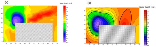
Figure 5.
(a) Simulated bed elevation contours around the square bridge abutment at t = 600 s under open channel condition; (b) Laboratory measured bed elevation contours around the square bridge abutment under open channel flow (flow direction is from left to right).
4.2. Local Scour around Semi-Circular Abutment under Open Channel Flow Condition
In a manner akin to the experimental setup, the numerical experiment was carried out utilizing an inflow velocity of 0.20 m/s and a uniform water depth of 0.19 m. It should be noted that the variability in the initial condition can be attributed to the presence of experimental data. The morphology and arrangement of the scour depression encompassing the semi-circular abutment exhibit similarities to the characteristics elucidated in the study conducted by Zhang et al. (2012) [39]. Figure 6a illustrates the numerical representation of the local scour that occurred around the semi-circular bridge abutment after 600 s, at which point the scouring severity reached a state of equilibrium. On the other hand, Figure 6b presents the experimental depiction of the local scour that developed around the semi-circular bridge abutment. Figure 6 illustrates that the maximum scour depth is 14 mm, as observed in both the numerical simulation and the experimental investigation. Nevertheless, the variation in the maximum scour depth and its spatial distribution can be attributed to the intricate nature of local scouring phenomena and the turbulent flow conditions upstream of the bridge abutment. The occurrence of this phenomenon is attributed to the principal vortex, which has its origin upstream of the abutment (20). The dissimilarity in the geometry of the scour region upstream and downstream is primarily attributed to the existence of a primary vortex and wake vortex in proximity to the abutment, along with their mutual influence. The scour hole upstream of the bridge abutment is primarily formed by the primary vortex, which exhibits characteristics similar to a half horseshoe vortex due to the utilization of only half of the abutment [20].
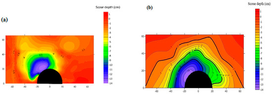
Figure 6.
(a) Simulated bed elevation contours around the semi-circular bridge abutment at t = 600 s under open channel condition; (b) Laboratory measured bed elevation contours around the square bridge abutment under open channel flow (flow direction is from left to right).
4.3. Local Scour around Square Abutment under Ice-Covered Flow Conditions
Figure 7a illustrates the simulated bed elevation contours surrounding the square bridge abutment in a channel bed with a median grain size (D50) of 0.50 mm under conditions of smooth ice-covered flow. In contrast, Figure 7b presents the experimental bed elevation contours around the same square bridge abutment in a channel bed, also under smooth ice-covered flow conditions. The similarity between numerical and experimental results is demonstrated in Figure 7a,b, where it can be observed that the maximum scour is concentrated in the same geographical area. In the experimental investigation, the highest recorded scour depth was measured to be 65 mm, whereas in the numerical simulation, the maximum scour depth was determined to be 66 mm. One factor contributing to this disparity is the buoyancy of the ice sheet. During the course of the investigations, it was observed that the model ice exhibited buoyancy on the water’s surface, resulting in slight variations in depth over time. In light of the constraints imposed by the numerical model employed for simulating the flow of ice, it was necessary to treat the ice cover as rigid within the numerical simulation. When an ice cover remains stationary, the limitation on the cross-sectional area leads to an augmentation in both the velocity and rate of sediment transport, thereby intensifying the process of local scouring [40]. The transport rate of suspended and bed-load sediment is lower for ice that is capable of floating compared to ice that is not capable of floating [41]. Although the maximum scour depth was the same for both the open channel flow condition and the smooth ice-covered flow condition, the scour pattern observed in the latter condition is more extensive.
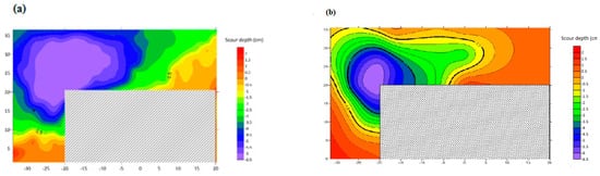
Figure 7.
(a) Simulated bed elevation contours around the square bridge abutment at t = 600 s under smooth ice-covered flow condition; (b) Laboratory measured bed elevation contours around the square bridge abutment under smooth ice-covered flow condition.
Figure 8a illustrates the simulated contours of bed elevation surrounding the square bridge abutment within a channel bed characterized by a D50 value of 0.50 mm. These simulations were conducted under conditions of uneven flow, specifically in the presence of ice cover. Figure 8b illustrates the experimental bed elevation contours surrounding the square bridge abutment situated in a channel bed characterized by a median grain size (D50) of 0.50 mm and an irregular flow pattern due to the presence of ice cover. In a manner akin to the experimental setup, the numerical experiment was carried out using an inflow velocity of 0.20 m/s and a consistent water depth of 0.19 m. At Point B (Figure 2), both laboratory experiments and numerical simulations observed a maximal scour depth of 80 mm. Nevertheless, the distribution of the scour field in the numerical simulation exhibits greater dispersion and irregularity as a result of the aforementioned concern regarding the buoyancy of the ice cover. In the laboratory setting, simulated ice was observed to exhibit free-floating behavior on the water’s surface during experiments. Moreover, the phenomenon of local scour near bridge piers is a considerably intricate process that is impacted by numerous variables. These variables encompass flow velocity, water depth, sediment grain size distribution, and the critical shield stress specific to each sediment type.
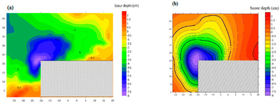
Figure 8.
(a) Simulated bed elevation contours around the square bridge abutment at t = 600 s under uneven ice-covered flow condition; (b) Laboratory measured bed elevation contours around the square bridge abutment under uneven ice-covered flow condition (flow direction is from left to right).
According to previous research [42], it has been observed that under conditions of uneven ice cover, the maximum flow velocity is found in closer proximity to the bottom compared to situations where the ice cover is smooth. Furthermore, erosion can serve as a means of alleviation by not only bringing the maximum velocity profile closer to the bed but also establishing an equilibrium between the heightened shear stress and the depth of the scour [43]. This leads to a differentiation between the depths of scouring observed under flat ice conditions and those observed under irregular ice conditions. This phenomenon is also the underlying cause for the irregular scour-deposition patterns observed on the channel bed when it is unevenly covered, as opposed to when it is covered by smooth ice or exposed to open channel flow. In a comparable manner, the presence of smooth ice cover during flow led to a less uniform distribution of scour patterns around bridge piers, as opposed to flow conditions observed in unobstructed channels.
4.4. Local Scour around Semi-Circular Abutment under Ice-Covered Flow Conditions
In Figure 9a, the bed elevation contours surrounding the semi-circular bridge abutment in the channel bed are illustrated. The simulation was conducted under uniform ice-covered steady flow conditions. Experimental bed elevation contours around the semi-circular bridge abutment in a channel bed with a median grain size (D50) of 0.50 mm under ice-covered smooth flow are illustrated in Figure 9b. Figure 9a,b demonstrate that the outcomes of the numerical simulation align closely with those obtained from the experimental inquiry. At Point E, both laboratory experiments and numerical simulations observed a maximal scour depth of 15 mm.
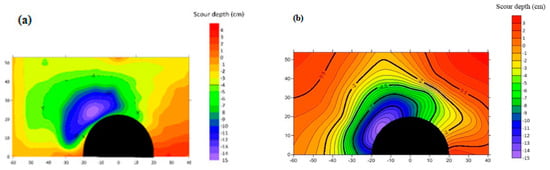
Figure 9.
(a) Simulated bed elevation contours around the semi-circular bridge abutment at t = 600 s under smooth ice-covered flow condition; (b) Laboratory measured bed elevation contours around the semi-circular bridge abutment under smooth ice-covered flow condition (flow direction is from left to right).
Figure 10a illustrates the simulated contours of bed elevation surrounding the semi-circular bridge abutment within a channel bed characterized by a D50 value of 0.50 mm. These simulations were conducted under conditions of uneven ice cover and steady flow. Figure 10b depicts the bed elevation contours obtained from experimental observations conducted on a semi-circular bridge abutment situated in a channel bed with a median grain size (D50) of 0.50 mm. The experiments were conducted under conditions of uneven ice cover and steady flow. In a manner akin to the experimental setup, the numerical experiment was carried out using an inflow velocity of 0.20 m/s and a consistent water depth of 0.19 m. At Point E, both laboratory experiments and numerical simulations yielded a maximal scour depth of 17 mm. The ice cover had an impact on the extent of erosion surrounding the abutment, in line with the findings of Valela et al. (2021) [44]. In scenarios characterized by uneven ice cover, the maximum scour depth exhibited greater magnitude compared to scenarios characterized by open channel and uniform ice cover. The presence of an uneven ice cover induces turbulence, resulting in a displacement of the maximum velocity towards the bed. This phenomenon can be attributed to the deeper scour near the abutment.
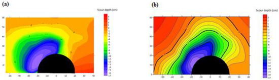
Figure 10.
(a) Simulated bed elevation contours around the semi-circular bridge abutment at t = 600 s under uneven ice-covered flow condition; (b) Laboratory measured bed elevation contours around the semi-circular bridge abutment under uneven ice-covered flow condition.
4.5. The Numerical Turbulent Energy Distribution around the Square Bridge Abutments
Figure 11a,b illustrates the turbulent energy and intensity in the context of open channel flow conditions. Note that turbulent energy refers to the kinetic energy associated with the chaotic and irregular motion of fluid particles in a turbulent flow. In turbulent flows, fluid particles move in a disorderly fashion, characterized by eddies, swirls, and vortices of varying sizes. This motion results in the constant exchange and redistribution of kinetic energy within the fluid. Turbulent energy is typically quantified using the turbulent kinetic energy (TKE) per unit mass or per unit volume of the fluid. It is a measure of the fluctuations in velocity within the turbulent flow. Mathematically, it can be expressed as TKE = (1/2) ∗ ρ ∗ u′2, where TKE is the turbulent kinetic energy, ρ is the fluid density, and u′ represents the turbulent velocity fluctuations. Turbulent intensity is a dimensionless parameter that quantifies the level of turbulence in a fluid flow relative to its mean velocity. It provides information about the variability of velocity within the flow and is often used in fluid dynamics and engineering applications. Turbulent intensity, denoted by I, is calculated as the root mean square (RMS) of the turbulent velocity fluctuations divided by the mean velocity. Based on the empirical observations, it can be inferred that the magnitudes of turbulent energy and turbulent intensity exhibit higher values at Point B of the square bridge abutment, as visually depicted in Figure 12. This can be attributed to the positive correlation between scour depth and turbulent energy, indicating that an increase in scour depth leads to a corresponding increase in turbulent energy. Experimental observations revealed that during the scouring process, finer particles exhibited a greater tendency to shift initially, while coarser sediment tended to accumulate in the vicinity of the square abutment and within the scour pit. The aforementioned procedure was iterated until the scour hole’s surface was enveloped by coarse sediment particles, thereby establishing a safeguarding stratum that impeded subsequent scouring. The state in which the rate of change in scour holes is negligible is referred to as the scour hole equilibrium state. Figure 13a illustrates the numerical representation of turbulent energy distribution surrounding the square bridge abutment in the presence of uniform ice conditions. In contrast, Figure 13b showcases the numerical contour of turbulent energy around the same square bridge abutment but under irregular ice conditions. Based on the data presented in Figure 13, it can be observed that the maximum values of turbulent energy exhibit a slight increase in the case of uneven ice-covered flow compared to smooth ice-covered flow. The findings of both numerical and experimental research regarding the maximal scour depths have been compiled and presented in Table 3. These results provide confirmation that the numerical model effectively simulated the scour depth values.
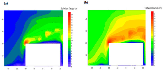
Figure 11.
(a) Numerical contour of turbulent energy around the square bridge abutment (b) Numerical contour of turbulent intensity (%) around the square bridge abutment.
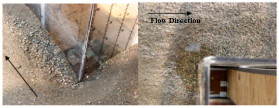
Figure 12.
Views of developed scour depth around the square bridge abutment.
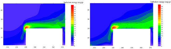
Figure 13.
(Left) Numerical contour of turbulent energy around the square bridge abutment under smooth ice-covered condition (Right) Numerical contour of turbulent energy around the square bridge abutment under uneven ice-covered condition.
Table 3.
Scour depth values gained from experiments and numerical values.
4.6. The Numerical Turbulent Energy Distribution around the Semi-Circular Bridge Abutments
The determination of the turbulent energy distribution around the piers during the experiment was hindered by experimental limitations. Nevertheless, given the successful simulation of scour depth and its strong correlation with turbulent energy, it is reasonable to anticipate that the numerical outcomes pertaining to turbulent energy distribution are reliable.
Figure 14a illustrates the spatial distribution of turbulent energy surrounding the semi-circular bridge abutment when subjected to open channel flow conditions. It is evident that the magnitude of turbulent energy is highest in the region between points D and E. Figure 14b illustrates the empirical perspective of the erosion occurring in the vicinity of the semi-circular bridge abutment. The numerical simulation clearly indicates that the region exhibiting the highest scour depth is also characterized by the highest turbulent energy. This finding illustrates that an increase in turbulent energy leads to a corresponding increase in scour depth. Figure 15a,b illustrate the numerical representation of the turbulent energy distribution surrounding the semi-circular bridge abutment in the presence of smooth and uneven ice-covered flow conditions, respectively. Based on the graphical representation, it can be observed that the turbulent energy exhibits its highest magnitude in the context of an irregular ice-covered flow. This finding suggests that this particular flow condition is associated with the most significant scour depth. Additionally, it is evident that the variability in ice cover has an impact on the flow characteristics and scour depth. Specifically, an uneven ice cover results in increased turbulence compared to a uniform ice cover, as well as greater scour depth. The presence of the primary vortex and flow acceleration on the left side of the semi-circular abutment, specifically near point E, leads to an increase in bed shear stress. This heightened stress ultimately triggers the onset of local scour in this particular area.
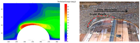
Figure 14.
(Left) Numerical contour of turbulent energy around the semi-circular bridge abutment; (Right) A view of developed scour depth around the semi-circular bridge abutment in the experiment.
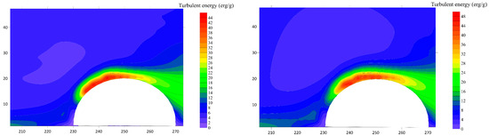
Figure 15.
(Left) Numerical contour of turbulent energy around the semi-circular bridge abutment under smooth ice-covered flow condition; (Right) Numerical contour of turbulent energy around the semi-circular bridge abutment under uneven ice-covered flow condition.
5. Conclusions
This study involved the execution of six numerical simulations to replicate the phenomenon of local erosion occurring in the vicinity of square and semi-circular bridge abutments. The study examined three different flow conditions: open channel flow, uniform ice cover, and uneven ice cover. The simulation results align with the empirical observations. The findings yielded significant insights into the examination of scour patterns, distribution of turbulent energy, and morphological alterations. The maximum scour depth for square bridge abutments is observed at the upstream corner of the abutment, where it is exposed to the incoming flow and experiences the highest levels of turbulent energy. Although the local scour pattern near bridge abutments remains consistent regardless of the flow cover, the turbulent energy intensity and scour depth are most pronounced when dealing with uneven flow conditions caused by ice cover. In relation to the semi-circular bridge abutments, the maximum scour depth is observed in close proximity to point E, which corresponds to an angle of 75 degrees with respect to the direction of the approaching flow. In this particular instance, it was observed that the square bridge abutment resulted in larger scour depths in comparison to the semi-circular abutment. Both experimental research and numerical simulations demonstrate a consistent pattern of turbulent energy distributions, wherein the highest magnitude is observed in the presence of uneven ice coverings. In this paper, artificial Styrofoam was utilized in the experimental study. Regarding the numerical aspect, it was explicitly explained that the ice cover is considered rigid due to constraints imposed by the employed numerical model. This decision was driven by the model’s limitations in simulating ice flow dynamics. When the ice cover remains stationary, this constraint on the cross-sectional area results in an increase in both velocity and sediment transport rate, intensifying the process of local scouring. The findings presented in this study demonstrate that the utilization of simulations can greatly contribute to the optimization of bridge abutment design.
Author Contributions
Conceptualization, methodology software, validation, writing—original draft preparation, visualization, M.R.N. Methodology, resources, supervision, writing—review and editing, P.W. Writing—review and editing, M.D. All authors have read and agreed to the published version of the manuscript.
Funding
The research is supported by the Discovery Grant of NSERC.
Data Availability Statement
All the data in the current work is accessible upon request.
Conflicts of Interest
The authors declare no conflict of interest.
References
- Barbhuiya, A.K.; Dey, S. Local scour at abutments: A review. Sadhana 2004, 29, 449–476. [Google Scholar] [CrossRef]
- Chang, H.H. Fluvial Processes in River Engineering; John Wiley: New York, NY, USA, 2008; 425p. [Google Scholar]
- Deng, L.; Cai, C.S. Bridge scour: Prediction, modeling, monitoring, and countermeasures. Pract. Period. Struct. Des. Constr. 2009, 15, 125–134. [Google Scholar] [CrossRef]
- Foti, S.; Sabia, D. Influence of foundation scour on the dynamic response of an existing bridge. J. Bridge Eng. 2010, 16, 295–304. [Google Scholar] [CrossRef]
- Zhu, S.; Levinson, D.M. Disruptions to transportation networks: A review. In Network Reliability in Practice; Springer: New York, NY, USA, 2012; pp. 5–20. [Google Scholar]
- Froehlich, D.C. Local scour at bridge abutments. In Proceedings of the 1989 National Conference on Hydraulic Engineering, New Orleans, LA, USA, 14–18 August 1989; pp. 13–18. [Google Scholar]
- Melville, B.W.; Chiew, Y.M. Time scale for local scour at bridge piers. J. Hydraul. Eng. 1999, 125, 59–65. [Google Scholar] [CrossRef]
- Coleman, S.E. Clearwater local scour at complex piers. J. Hydraul. Eng. 2005, 131, 330–334. [Google Scholar] [CrossRef]
- Dey, S.; Sarkar, A. Scour downstream of an apron due to submerged horizontal jets. J. Hydraul. Eng. 2006, 132, 246–257. [Google Scholar] [CrossRef]
- Shen, H.T.; Yapa, P.D. Flow resistance of river ice cover. J. Hydraul. Eng. 1986, 112, 142–156. [Google Scholar] [CrossRef]
- Kwan, R.T.; Melville, B.W. Local scour and flow measurements at bridge abutments. J. Hydraul. Res. 1994, 32, 661–673. [Google Scholar] [CrossRef]
- Zabilansky, L.J.; White, K.D. Ice-cover effects on scour in narrow rivers. In Proceedings of the Third International Conference on Remediation of Contaminated Sediment, New Orleans, LA, USA, 11–14 February 2005; pp. 24–27. [Google Scholar]
- Wu, P.; Balachandar, R.; Sui, J. Local scour around bridge piers under ice-covered conditions. J. Hydraul. Eng. 2015, 142, 04015038. [Google Scholar] [CrossRef]
- Wu, P.; Hirshfield, F.; Sui, J.Y. Local scour around bridge abutments under ice covered conditions-an experimental study. Int. J. Sediment. Res. 2015, 30, 39–47. [Google Scholar] [CrossRef]
- Namaee, M.R.; Sui, J.; Wu, Y.; Linklater, N. Three-dimensional numerical simulation of local scour around circular side-by-side bridge piers with ice cover. Can. J. Civ. Eng. 2021, 48, 1335–1353. [Google Scholar] [CrossRef]
- Toombes, L.; Chanson, H. Numerical limitations of hydraulic models. In Proceedings of the 34th IAHR World Congress, 33rd Hydrology and Water Resources Symposium and 10th Conference on Hydraulics in Water Engineering, Brisbane, Australia, 26 June–1 July 2011; pp. 2322–2329. [Google Scholar]
- Richardson, J.E.; Panchang, V.G. Three-dimensional simulation of scour-inducing flow at bridge piers. J. Hydraul. Eng. 1998, 124, 530–540. [Google Scholar] [CrossRef]
- Vasquez, J.A.; Walsh, B.W. CFD simulation of local scour in complex piers under tidal flow. In Proceedings of the 33rd IAHR Congress: Water Engineering for a Sustainable Environment, Vancouver, BC, Canada, 9–14 August 2009. [Google Scholar]
- Kim, H.S.; Nabi, M.; Kimura, I.; Shimizu, Y. Numerical investigation of local scour at two adjacent cylinders. Adv. Water Resour. 2014, 70, 131–147. [Google Scholar] [CrossRef]
- Dey, S.; Barbhuiya, A.K. Time variation of scour at abutments. J. Hydraul. Eng. 2005, 131, 11–23. [Google Scholar] [CrossRef]
- Melville, B.W. Local scour at bridge abutments. J. Hydraul. Eng. 1992, 118, 615–631. [Google Scholar] [CrossRef]
- Omara, H.; Elsayed, S.M.; Abdeelaal, G.M.; Abd-Elhamid, H.F.; Tawfik, A. Hydromorphological Numerical Model of the Local Scour Process Around Bridge Piers. Arab. J. Sci. Eng. 2019, 44, 4183–4199. [Google Scholar] [CrossRef]
- Hatton, K.A.; Foster, D.L.; Traykovski, P.; Smith, H.D. Numerical Simulations of the Flow and Sediment Transport Regimes Surrounding a Short Cylinder. IEEE J. Ocean. Eng. 2007, 32, 249–259. [Google Scholar] [CrossRef]
- Amini, A.; Parto, A.A. 3D Numerical Simulation of Flow Field around Twin Piles. ACTA Geophys. 2017, 65, 1243–1251. [Google Scholar] [CrossRef]
- Daneshfaraz, R.; Ghaderi, A.; Sattariyan, M.; Alinejad, B.; Asl, M.M.; Di Francesco, S. Investigation of Local Scouring around Hydrodynamic and Circular Pile Groups under the Influence of River Material Harvesting Pits. Water 2021, 13, 2192. [Google Scholar] [CrossRef]
- Nielsen, A.W.; Liu, X.F.; Sumer, B.M.; Fredsoe, J. Flow and Bed Shear Stresses in Scour Protections around a Pile in a Current. Coast. Eng. 2013, 72, 20–38. [Google Scholar] [CrossRef]
- Choufu, L.; Abbasi, S.; Pourshahbaz, H.; Taghvaei, P.; Tfwala, S. Investigation of Flow, Erosion, and Sedimentation Pattern around Varied Groynes under Different Hydraulic and Geometric Conditions: A Numerical Study. Water 2019, 11, 235. [Google Scholar] [CrossRef]
- Hirt, C.W.; Nichols, B.D. Volume of fluid (VOF) method for the dynamics of free boundaries. J. Comput. Phys. 1981, 39, 201–225. [Google Scholar] [CrossRef]
- Hirt, C.W.; Sicilian, J.M. A porosity technique for the definition of obstacles in rectangular cell meshes. In Proceedings of the 4th International Conference on Numerical Ship Hydrodynamics, Washington, DC, USA, 24–27 September 1985; pp. 1–19. [Google Scholar]
- Flow Sciences Inc. FLOW-3D User’s Manual Version 11.1; Flow Sciences Inc.: Santa Fe, NM, USA, 2015. [Google Scholar]
- Yakhot, V.; Orszag, S.A.; Thangam, S.; Gatski, T.B.; Speziale, C.G. Development of turbulence models for shear flows by a double expansion technique. Phys. Fluids A 1992, 4, 1510–1520. [Google Scholar] [CrossRef]
- Launder, B.E.; Spalding, D.B. The Numerical Computation of Turbulent Flows. Comput. Methods Appl. Mech. Eng. 1974, 3, 269–289. [Google Scholar] [CrossRef]
- Zhang, Q.; Zhou, X.L.; Wang, J.H. Numerical investigation of local scour around three adjacent piles with different arrangements under current. Ocean. Eng. 2017, 142, 625–638. [Google Scholar] [CrossRef]
- Mastbergen, D.R.; Von den Berg, J.H. Breaching in fine sands and the generation of sustained turbidity currents in submarine canyons. Sedimentology 2003, 50, 625–637. [Google Scholar] [CrossRef]
- Soulsby, R.L.; Whitehouse, R.J.S. Threshold of sediment motion in coastal environments. In Pacific Coasts and Ports’ 97, Proceedings of the 13th Australasian Coastal and Ocean Engineering Conference and the 6th Australasian Port and Harbour Conference, Melbourne, Australia, 18–21 April 1997; ; Centre for Advanced Engineering, University of Canterbury: Christchurch, New Zealand, 1997; Volume 1, p. 145. [Google Scholar]
- Meyer-Peter, E.; Müller, R. Formulas for bed-load transport. In Proceedings of the IAHSR 2nd Meeting, Stockholm, Sweden, 7–9 June 1948. appendix 2. IAHR. [Google Scholar]
- Nielsen, P. Coastal Bottom Boundary Layers and Sediment Transport; World Scientific Publishing Company: Singapore, 1992; Volume 4. [Google Scholar]
- Van Rijn, L. Sediment transport, Part I: Bed load transport. J. Hydraul. Eng. 1984, 110, 1431–1456. [Google Scholar] [CrossRef]
- Wu, P.; Hirshfield, F.; Sui, J.; Wang, J.; Chen, P.P. Impacts of ice cover on local scour around semi-circular bridge abutment. J. Hydrodyn. Ser. B 2014, 26, 10–18. [Google Scholar] [CrossRef]
- Tang, J.H.; Puspasari, A.D. Numerical simulation of local scour around three cylindrical piles in a tandem arrangement. Water 2021, 13, 3623. [Google Scholar] [CrossRef]
- Zhang, H.; Nakagawa, H.; Mizutani, H. Bed morphology and grain size characteristics around a spur dyke. Int. J. Sediment Res. 2012, 27, 141–157. [Google Scholar] [CrossRef]
- Ettema, R.; Kempema, E.W. River-Ice Effects on Gravel-Bed Channels. In Gravel-Bed Rivers: Processes, Tools, Environments; John Wiley & Sons: Hoboken, NJ, USA, 2012; pp. 523–540. [Google Scholar]
- Sui, J.; Wang, J.; He, Y.; Krol, F. Velocity profiles and incipient motion of frazil particles under ice cover. Int. J. Sediment. Res. 2010, 25, 39–51. [Google Scholar] [CrossRef]
- Hains, D.; Zabilansky, L.J.; Weisman, R.N. An experimental study of ice effects on scour at bridge piers. In Proceedings of the Cold Regions Engineering and Construction Conference and Expo, Edmonton, AB, Canada, 16–19 May 2004. [Google Scholar]
Disclaimer/Publisher’s Note: The statements, opinions and data contained in all publications are solely those of the individual author(s) and contributor(s) and not of MDPI and/or the editor(s). MDPI and/or the editor(s) disclaim responsibility for any injury to people or property resulting from any ideas, methods, instructions or products referred to in the content. |
© 2023 by the authors. Licensee MDPI, Basel, Switzerland. This article is an open access article distributed under the terms and conditions of the Creative Commons Attribution (CC BY) license (https://creativecommons.org/licenses/by/4.0/).