The Influence of the Main Factors on the Accuracy of Hydrological Modelling of Flooded Lands

Abstract

This paper proposes a general methodological approach to hydrological modeling for determining the areas of flooded land in the plain part of the Dniester riverbed, the second largest river in Ukraine. The purpose of the study is the selection of parameters for modeling flooded zones in the plain section of the Dniester riverbed, taking into account the rising water level caused by the freshet that occurred in the western part of Ukraine on 22–24 June 2020. The proposed study examines the workflow of hydrological modeling of the flooded land zone and the main components of this scheme: the construction of the DTM, considering the roughness of the riparian territory by Manning’s coefficients, and indications of water rise. In the experiment, the influence of DTM reproduction resolution and Manning coefficients was analyzed, and their optimal values were selected, which allowed obtaining the parameters of hydrological modeling with a higher probability. The identified flooding areas were tested using a high-resolution space image during the flood in June 2020. The distance between the profiles affects not only the value of the modeling area but also their detail. The accuracy of the modeled flooded area is 5.1% for a 5 m interval between the profiles, 6.9% for 50 m, 8.2% for 100 m, and 10.8% for 200 m. These results allow determining the degree of influence of the distance between intervals on the modeling accuracy. Using different values of Manning’s coefficients for individual sections with different bedding surfaces and the selected spacing between profiles, which was 50 m, the accuracy of the modeling was investigated. After the modelling, the simulated flood areas were obtained in vector form, which allows for determining their areas and comparing them with the test flooded area. In the presented research, the RMSE of determining the flooded areas is about 5%. The test area of 600.6 hectares was determined with an accuracy of 0.8%.

1. Introduction

In recent years in Ukraine, catastrophic freshets and floods have increased significantly. The destructive power of these phenomena is constantly growing. Considering their negative impact on anthropogenic systems and associated social and economic losses, hydrological modeling is essential for modeling applied problems. In particular, it is taken into account in hydro-technical construction, the design of bridges and river crossings, the building of gas transmission lines, the assessment of potentially dangerous sections of riverbeds, the study of the consequences of flood phenomena, and the establishment of protection zones in land management. Hydrological modeling makes it possible to estimate the scale of flooding at different levels of water rise and make forecasts of these phenomena. Forecasting flood magnitude is essential for solving economic, environmental, and social problems and remains a fundamental challenge for hydrologists [1]. In Europe, the most serious floods are often transboundary in nature and can be managed by several responsible authorities in different countries and administrative areas. In the context mentioned above, the European Parliament’s 2007/60 EC directive was adopted, which was transformed in all member states into legal provisions and laws with the aim of the most effective prevention of floods. It requires Member States to conduct a preliminary flood risk assessment and prepare flood hazard maps, risk maps, and flood risk management plans for high-risk areas [2]. Multinational cooperation between countries using a shared waterway requires special studies and agreements. In this regard, the European Flood Awareness System (EFAS) was established, which operates on a pan-European scale to provide harmonised flood forecasts and relevant information to the majority of hydrological services responsible for flood forecasting in Europe, as well as to the European Civil Defence. EFAS aims to develop a prototype early flood forecasting system capable of simulating the average flood risk in Europe within 3–10 days.

To create a system for improving the protection of the economy, environment, and society from specific threats, especially floods and freshets, the ISOK project “Program system for the protection of the country from extraordinary threats” has been developed in Poland. The project identifies areas with a threat to life and property, which helps limit economic expansion in areas related to the exploitation of river systems. The final result of the activity is an electronic information platform that contains the necessary registration guides as an essential tool for anti-crisis management [3,4,5].

Assessments of flood phenomena, including flooded land, are based on the use of Earth remote sensing and GIS technologies, as well as field research data, which enable regular monitoring of the state of territories and provide comprehensive coverage, repeatability, and high-speed obtaining and processing of information. In addition, using remote sensing and GIS technologies opens up new opportunities for obtaining real-time flood zone forecasts, preliminary assessments of flood scales, identification of the most suitable locations for protective structures, and monitoring of coastal areas.

The purpose of the study is the selection of parameters for modeling flooded zones in the plain section of the Dniester riverbed, taking into account the rising water level caused by the freshet that occurred in the western part of Ukraine on 22–24 June 2020.

Hydrologists have developed a series of conceptual models and applied them to operations such as assessing water resources and predicting floods. Mathematical models are used to simulate water flow in channels, which, under certain assumptions, are different approximations of the shallow water equations, i.e., the Saint-Venant equations. These are a system of hyperbolic partial differential equations.

Morphological measurements and hydraulic characteristics of riverbeds are determined using optimization methods, which simplify the Saint-Venant equations to a dimensionless form and express them in differential form. In all cases, satisfactory results can be achieved by searching for unknown coefficients in the original equations and the calibration model. A classic work describing an example of solving the inverse problem of the Saint-Venant equations is the article by V. I. Koren and L. S. Kuchment [6].

An overview of the main processes of hydrological modeling is discussed in the work [7]. When hydrological modeling is essential to choose a model that depends on the type of channel, morphometric characteristics, and substrate. To account for the influence of the substrate, researchers use Manning’s equations in their models. Manning’s equation is one of the most widely used formulas for calculating flow velocity in open channels. It calculates flow velocity as a function of hydraulic radius, slope, and roughness coefficient, which quantitatively determine the slowing effect of the inundation layer. This is not the only formula for quantifying flow velocity, but it is most commonly used to estimate the roughness of the bed and floodplain. The article [8] studies the Manning roughness coefficient (n) and seasonal dynamics based on a one-dimensional hydrological model. The results showed that using dynamic n can improve the modeling of hydrological models, especially on slopes. Today, there is a gap in the scientific literature regarding the variability of the roughness coefficient, and many studies have claimed that the coefficient should be studied more closely. Although many factors affect the Manning roughness coefficient, the presence and variability of vegetation in the channel are likely one of the least studied factors. The importance and significance of vegetation for hydrological calculations are mentioned in publications [9,10,11].

Modern GIS technologies are essential to implementing hydrological research. In several countries, the active implementation of GIS technologies in hydrological science and practice began in the first half of the 1990s [12].

Initially, the development of hydrological models was intended only to solve specific problems in a particular field or watershed, so most hydrological models can only be applied under specific conditions [13].

Different viewpoints are evidence that the diversity of classifications of hydrological models boils down to four primary data points: the model basis, spatial representation, temporal representation, and solution method. The work [14] presents a classification of numerical watershed models, considering five main factors: model geometry, input data, main equations, initial and boundary conditions, and output data.

Hydrological models require a proper description of the modeling object’s morphometric and hydrological characteristics. Two generally accepted characteristics that models should demonstrate are simplicity and relevance to the problem under consideration, i.e., the model should be simple and should correspond to its purpose.

Several thematic studies have used a one-dimensional model to demonstrate its capabilities for analyzing floods. The distance between cross-sections, the selection of a river’s cross-section profile, and the influence of vegetation in riparian areas have been investigated [15,16].

Topographical data and their resolution are used for accurate two-dimensional modeling [17]. However, computation costs increase exponentially as resolution increases. A study [18] was conducted on a two-dimensional model with grid resolutions ranging from 2.5 to 50 m, and better results were obtained using a grid with smaller intervals. Also, the Digital Terrain Model (DTM) source is very important for hydrodynamic analysis results [19]. Downgrading the model resolution due to a lower resolution can cause unreliable results [20].

Various intervals between cross-sections using the DTM were tested in the HEC-RAS module [21]. A minimal influence was observed between different distances of cross-sections on the modeling results. In the work [22], the author created a different number of cross-sections based on the DTM with small intervals between them. It was found that adding additional cross-sections to the one-dimensional hydrological model only sometimes improves the accuracy of the model after reaching a satisfactory interval, depending on the geometry of the riverbed, the physical wave of the flood, and the form of the tide.

During the study on the impact of vegetation in the riverbed on the geometry of the cross-profile, it was found that as the slope of the river decreases downstream, the velocity also decreases due to the influence of the river vegetation, resulting in river widening [23].

The problem of determining changes in riverbeds, conducting their monitoring, managing flood events, and studying threats and economic and ecological losses to minimize them remains relevant, as evidenced by several state and administrative directives and recommendations adopted in various countries and numerous scientific research papers.

2. Materials and Methods

2.1. Theoretical Approaches to Hydrological Modelling

Hydrology uses a complex mathematical method based on the laws of mathematics, physics, and hydrological and geomorphological features of a water body to model the hydraulic characteristics of a stream. For this purpose, mathematical physics is widely used, which studies real-world processes using mathematical models based on the laws of physics [24,25].

Most researchers use Saint-Venant’s differential equation as a mathematical model to describe the unstable, smooth variational process of water flowing in open channels. There are many different forms of these equations. Chugaev [26] presents them in the form of flow continuity. Equation (1) is described as follows:

$$\frac{dQ}{ds}+\frac{dW}{dt}=q$$

(1)

where 𝑄—water flow rate; W—cross-section area; 𝑡—time scale; 𝑠—distance scale; q—lateral inflow per unit length of the river.

The second equation is the equation of motion, which determines the hydraulic slope of the flow between cross-sectional profiles as a result of the hydraulic resistance of the channel:

$$i-\frac{\partial H}{\partial s}=\frac{\alpha }{g}\left(V\frac{\partial V}{\partial s}+\frac{\partial V}{\partial t}\right)+\frac{V^2}{C^{2}R}+\frac{dV}{gW}$$

(2)

where i—bottom slope, H—flow depth, V—flow velocity, R—hydraulic radius, 𝐶—hydraulic drag coefficient, 𝑔 = 9.81—free fall acceleration, and α—Coriolis coefficient associated with the uneven distribution of the flow velocity along the cross-section, usually α = 1.1.

Equations (1) and (2) are incomplete models of the unsteady movement of open flows. Surface effects, flow curvature, the vertical component of accelerations, and other factors are not considered here. The solution is based on finite difference methods that describe the model as a set of points, or nodes. Areas of continuous variations of parameters (segments, rectangles, etc.) are replaced by a finite (discrete) set of points (nodes). If the problem is solved and its solution approaches the solution obtained from differential equations, it is considered an approximate solution to the original problem [27].

2.2. Manning’s Coefficients and Their Significance in Modelling

The Manning’s coefficient is a key parameter required for channel capacity calculation. Estimating Manning’s roughness coefficient is essential for modeling open channel flows. As an empirical parameter, the roughness coefficient actually includes components of surface friction resistance, shape resistance, wave resistance, and resistance due to flow instability [14].

Although the conditions for modeling unsteady flow may require a special approach to the definition of the roughness slope, most work in this area considers using the Manning Equation (3) to model indirect constant uniform flow [28].

$$V=\frac{\mu }{n}{R}^{2/3}{S}_e^{1/2}$$

(3)

where μ—is a conversion factor (μ = 1 for SI units and μ = 1.49 for English units), V—the cross-sectional average velocity, n—Manning’s roughness coefficient, R—hydraulic radius, S_e—energy slope of the channel.

If a large number of calculations are required when using the Manning equation, it is sometimes convenient to use the term “transit” as described by Equation (4):

$$K=\frac{\mu }{n}A{R}^{2/3}$$

(4)

where K is the channel capacity and A is the cross-sectional area of the channel.

The values of Manning’s n coefficients, depending on the factors affecting the roughness, can be found in the book [29].

Several factors affecting the roughness coefficient were mentioned [9]. One of these factors is surface roughness. It is the material that forms the wetted perimeter, such as the size and shape of stones on the bed and banks of the channel. While fine-grained material will result in a low Manning’s coefficient value, coarser material will indicate an increase in the value.

The roughness values for floodplains can be significantly different from the values for channels. Therefore, the roughness value for floodplains should be determined independently from the channel. The coefficient value can be applied to a single cross-sectional profile typical of the site, but it should consider the roughness of the entire area that runs along the line of the cross-sectional profile. Where two or more cross-sections are considered, the range applicable to any one section shall be considered to extend to half the distance to the next section.

The HEC-RAS 5.0 module is based on the principles of a one-dimensional hydrological model for flood research. It is an integrated software system designed for interactive use in a multi-tasking environment. The system has a graphical interface, separate analysis components, data storage and management, graphical and reporting tools. The main computational procedure is based on solving a one-dimensional energy equation. Energy losses are estimated using Manning’s roughness coefficient, which considers the type of the underlying surface [30].

In the one-dimensional model, the morphometric characteristics of the flow are averaged over the width and depth and considered along the x-axis. Considering the small width of the Dniester river channel (up to 120 m), we applied a one-dimensional model of the steady flow of water according to the Saint-Venant equations. They are solved using the numerical method in the HEC-RAS module.

2.3. Block Diagram of Hydrological Modelling

The scheme of hydrological modeling using the HEC-RAS module was developed by the authors and is shown in Figure 1.

The calibration parameters of the model are the distances between the transverse profiles, which define the height component of the model, and the roughness coefficient of the riverbed and the riparian area. Manning’s equations indicate the dependence of the flow velocity on the shape and size of the cross-sectional profile and the roughness of the riverbed walls.

2.4. Modeling of Flood Zones in the Plain Part of the Dniester Riverbed Hydrology

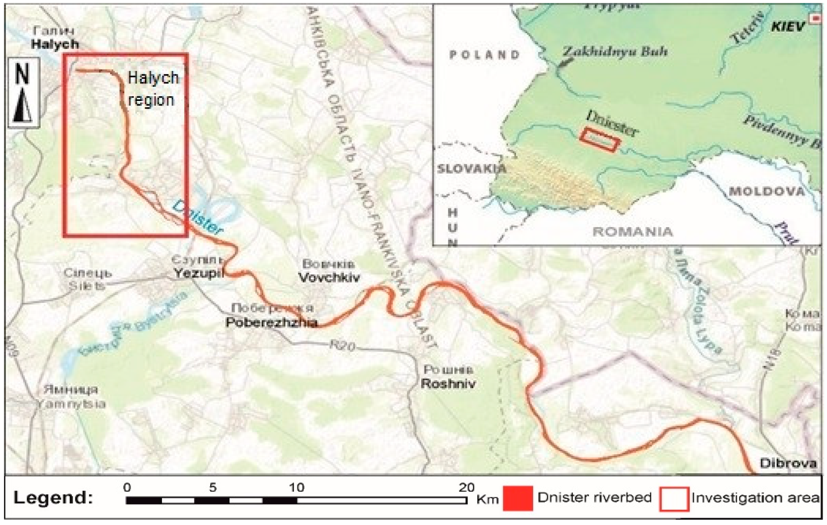
Characterization of the Dniester riverbed section. The plain part of the Dniester River channel is located near the city of Halych, Ivano-Frankivsk Oblast, Ukraine. The river flows on the border of two geological structures—the Precarpathian Basin and Volyn-Podilsk Upland. The visual location of this part of the riverbed is shown in Figure 2.

The width of the riverbed in this part is 100–120 m and is characterized by high tortuosity. The riverbed slope is 0.34 m/km. The depth of the riverbed varies between 2 and 4 m, and the average flow velocity is 0.8 m/s. Precipitation averages 450–700 mm/year, and the average monthly water discharge is 153 m³/s. The main morphometric, meteorological, and hydrological characteristics of the Dniester River are presented in

Table 1. Main morphometric and hydrological characteristics of the site study.

Parameter	Value
Length, km	9
Stream slope, m/km	0.34
Average monthly water consumption, m3/s	153
Runoff modulus, L/s per km2	10.4
Average river width, m	100–120
Average river depth, m	2–4
Flow rate, m/s	0.8–1
Average sediment diameter, mm	1
Average floodplain width, m	2010

.

Below the town of Halych, large left tributaries flow into the Dniester: Zolota Lypa, Hnyla Lypa, Koropets, etc. The valley is a flat, slightly hilly plateau about 2010 m wide. A prominent feature of the Dniester River is the large amount of sediment transported along the riverbed. This is primarily due to the mountainous nature of the river’s feeding, where coarse sediments such as pebbles and gravel enter the riverbed mainly from the right Carpathian tributaries (Limnytsia, Stryi, Bystrytsia, etc.). The Dniester is primarily fed by rain and snowmelt. The local soils have higher permeability rates than the Carpathian part of the Dniester basin, which indicates a more substantial influence of groundwater flow on the river flow.

2.5. Theoretical Approaches to Hydrological Modeling

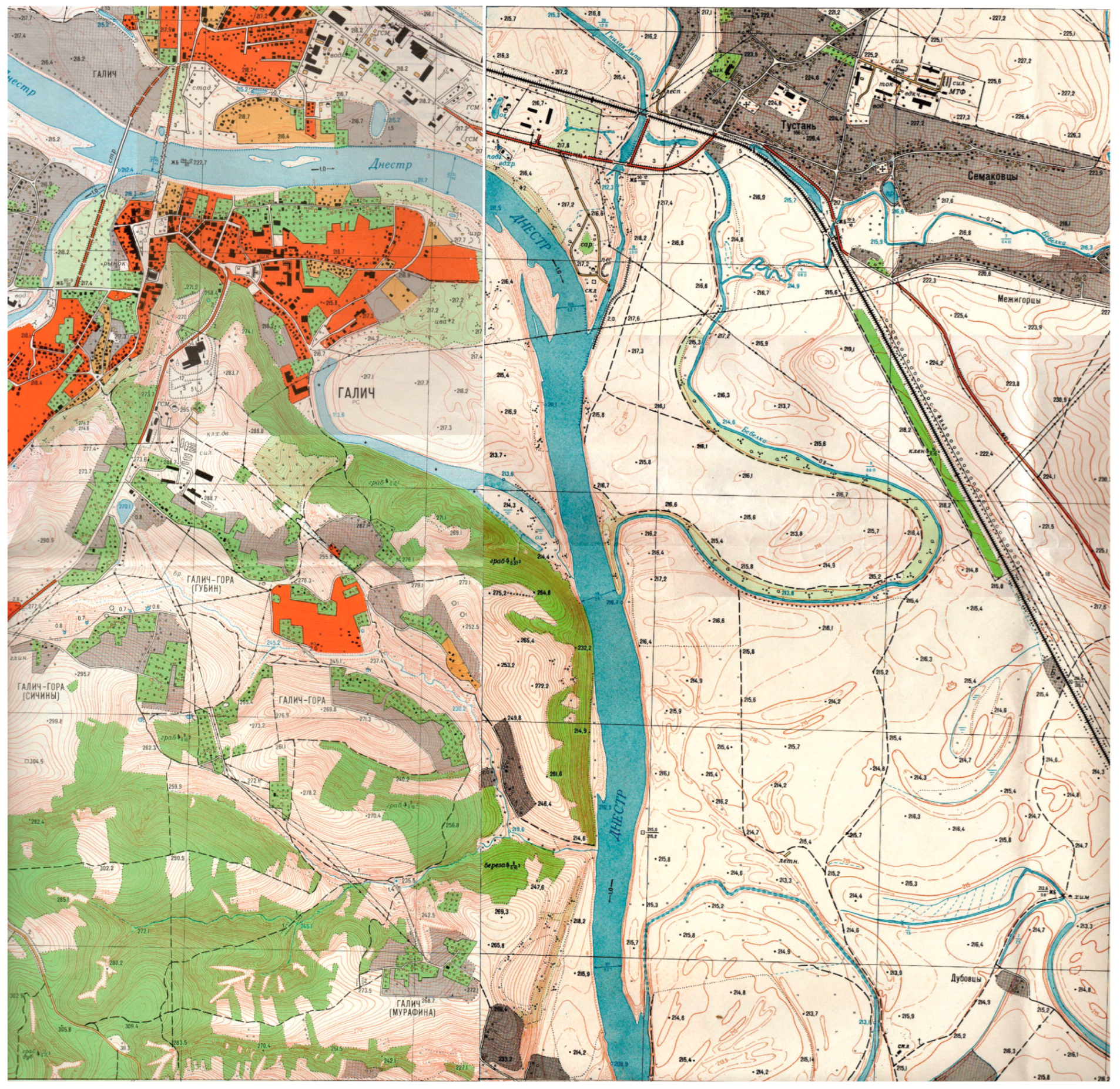
Under the structural scheme of hydrological modeling, the DTM was constructed by the cartometric method based on the processing of topographic maps at a scale of 1:10,000 with a contour interval of 1 m. A fragment of the topographic map is shown in Figure 3. In [31], it is established that topographic maps of a 1:10,000–1:2000 scale with a contour interval of 1–0.5 m should be used to determine the area of flooded land.

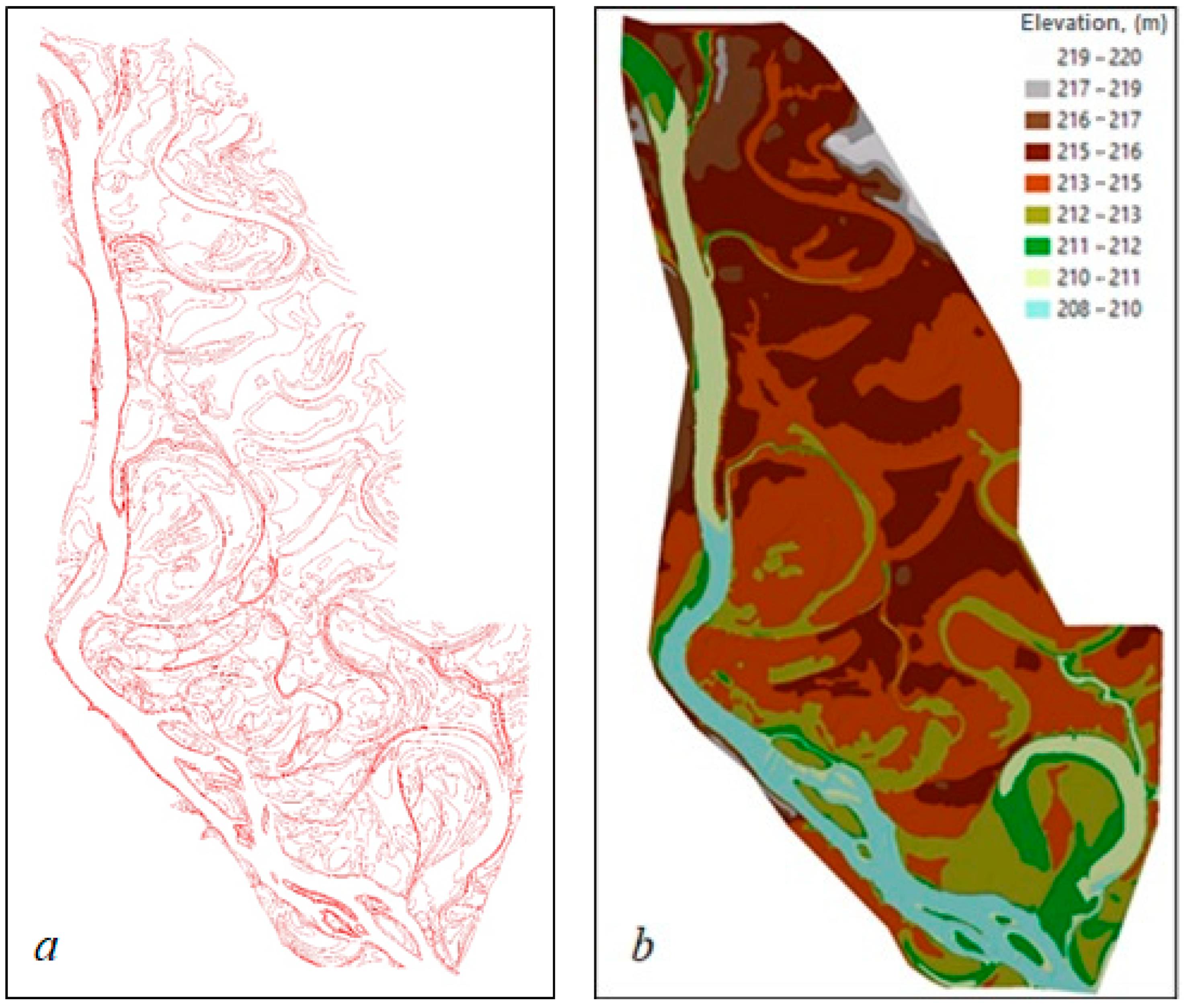
The map was used to vectorize contour lines and elevation points. A fragment of the vectorized contour lines is shown in Figure 4a. The heights of the contour lines were used to build a DTM and represent the model in raster form. Figure 4b shows the digital elevation model created by the cartometric method.

Flooding modeling was carried out on the territory characterized by a significant number of microforms of relief, located at a distance of 2 km from the city of Halych and extending down the riverbed for 9 km. Due to the constant floods in the Carpathian region, hydraulic works were carried out and the channel was straightened and diked, which is clearly visible on the map from 2010. Therefore, the horizontal displacements in this section are relatively small. The difference in elevation is 12 m. The accuracy of the DTM is 1 m horizontally and 0.3 m vertically.

Particular attention is paid to the study of flood dynamics and channel displacements after flood events. River channel displacements are of practical importance for selecting hydraulic engineering construction sites and construction technologies, for determining protected land zones, and for hydrological modeling to determine revised Manning’s coefficients that will take into account changes in the bedding surface, especially the impact of vegetation.

3. Results

3.1. Determination of Manning’s Coefficients

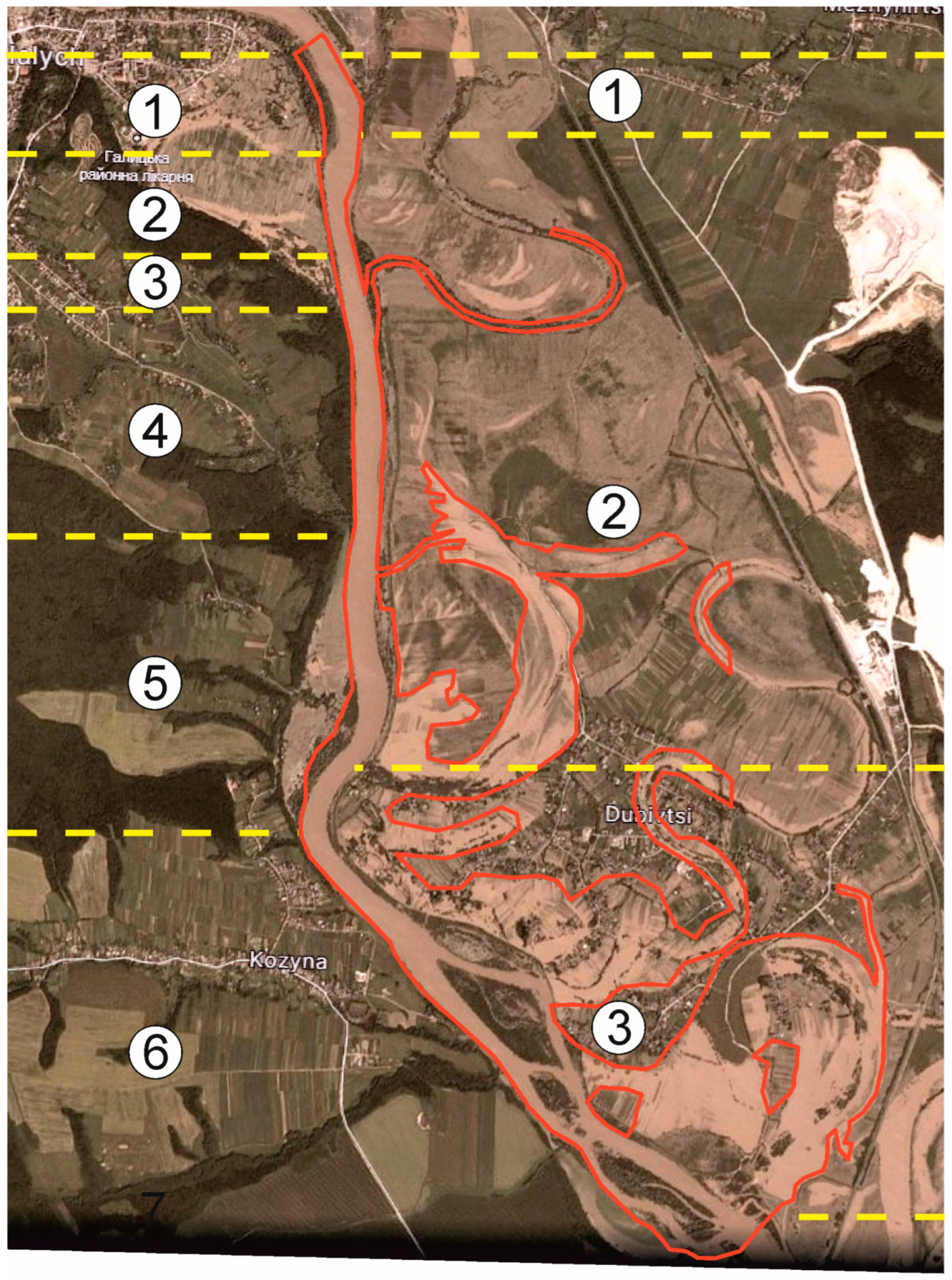
Roughness coefficients represent the resistance of the underlying surface to flood flows in channels and floodplains. The results of calculations by the Manning formula are used in floodplain management, flood insurance studies, and the design of bridges and highways across floodplains. To consider the type of underlying surface and test the accuracy of determining the area of flooded land, an image from PlanetScope (resolution 3 m/pixel) on 25 June 2020 was used.

Based on the satellite image, the flooded areas were vectorized, and sections with the same land cover/use were identified, as shown in Figure 5.

To estimate the accuracy of the determined flooded area, the following Formulas (5) and (6) were used [32]:

$$m_s=m_t\sqrt{S}\sqrt{\frac{1+k^2}{2k}}$$

(5)

$$m_t=m_x\sqrt{2}$$

(6)

where m_t—accuracy of distance determination; k—number of turning points; m_х—linear pixel size.

The flooded area is 600.6 hectares; the number of turning points is 49; the linear pixel size is 3 m. The accuracy of the flooded area is 4.94 hectares (0.82%).

The determined values of the coefficients for each type of bedding surface are presented in

Table 2. Minimum, average, and maximum values of Manning’s coefficients for the studied channel section.

Section Number	Characteristics of the Territory	Minimum	Average	Maximum
Right bank
1	Dense willows in summer	0.110	0.150	0.200
2	Tall grass	0.030	0.035	0.050
3	Dense willows in summer	0.110	0.150	0.200
4	Dense forest, several fallen trees, small undergrowth, flood level below branches	0.080	0.100	0.120
5	Low grass	0.025	0.030	0.035
6	Ripe row crops	0.025	0.035	0.045
Left bank
1	Dense willows in summer	0.110	0.150	0.200
2	Low grass	0.025	0.030	0.035
3	Ripe row crops	0.025	0.035	0.045

[33]. They can be used as a reference level for different kinds of streams. The table contains the minimum, average, and maximum values of Manning’s coefficients for different types of bedding. Still, for modeling floods associated with a particular river, the modeling determines the kind of bedding for each selected profile line on the left and right banks. The data for the channel itself is entered separately.

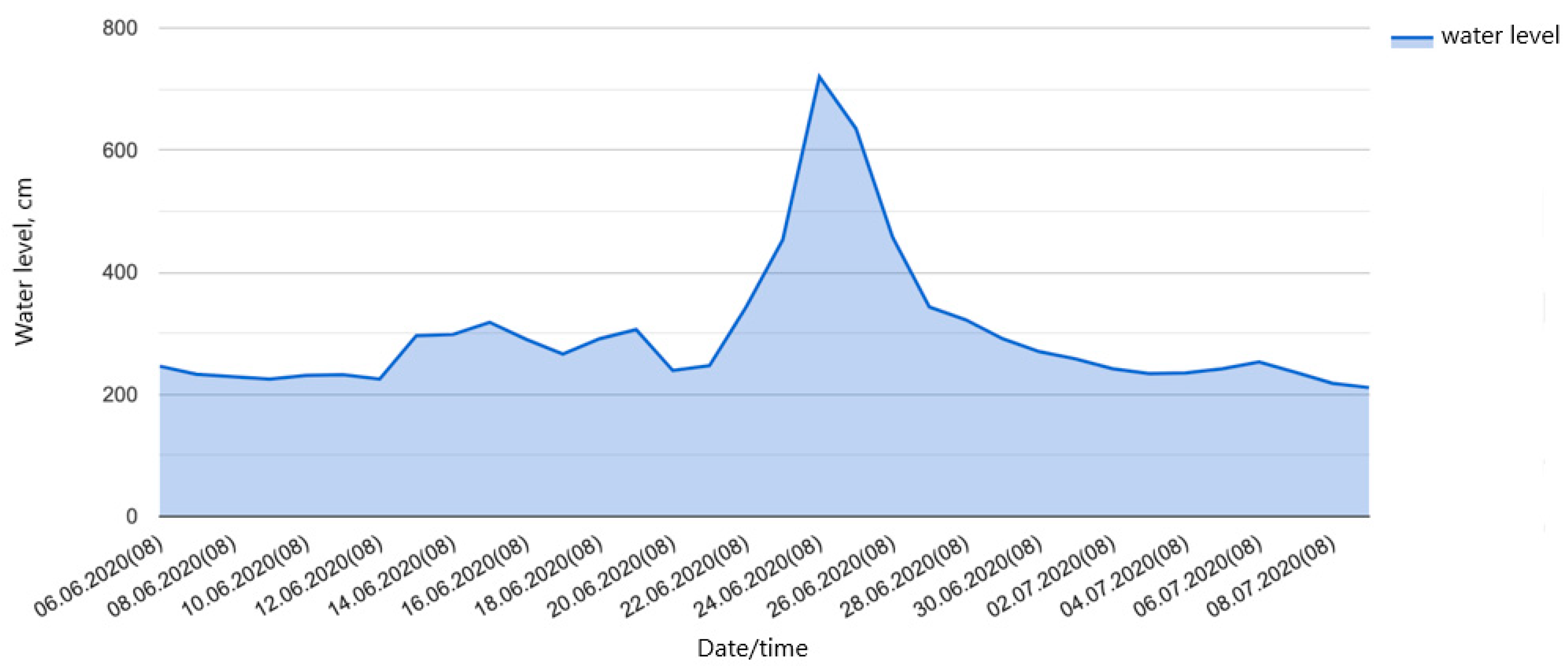
3.2. Determination of the Water Level

The data for determining the water level is obtained from hydrometeorological stations. Such a post is located near the study area in Halych. Modern technologies use automated systems of hydrometeorological stations, which allow them to take into account not only the amount of precipitation but also the morphometric characteristics of the area. The numerical values of the water level in the channel were obtained from the hydrological plot (Figure 6).

3.3. Determination of Hydrological Model Parameters

For accurate modeling, it is important to select the proper distance between the transverse profiles of the DTM and determine Manning’s coefficients for different types of bedding surfaces, taking into account their changes. In determining the distance between DTM cross sections, transverse profiles should be set in those sections of the stream where there are changes in water flow, slopes, changes in the shape of the channel cross-sectional profile, or roughness, at the beginning or end of dams, bridges, dams, etc.

The cross sections should cover the entire floodplain and be constructed from the left bank to the right bank perpendicular to the direction of flow. In addition, they should not extend beyond the DTM boundary, as the attribute table will not be able to be populated with elevation values.

Cross-sectional spacing also depends on flow length, slope, and cross-sectional shape uniformity. Sections should be spaced closely enough to account for significant changes in the hydraulics or geometry of the stream, such as changes in slope, cross-sectional shape, roughness, or hydraulic structure. Large, homogeneous rivers with low slopes usually require fewer cross-sections per kilometer.

Each profile is assigned a serial number corresponding to the distance from the downstream boundary of the channel section and information about the shoreline. The primary step in preparing cross-sectional profiles is to fill in their attribute tables with absolute elevation values and assign roughness values for the riverbed and banks (Manning’s coefficients) [34].

The dimensions of the profiles form the boundaries of the area to be modeled, so they must extend far enough on both sides of the channel to cover all potentially hazardous areas. Since the flooded zones are known in advance, the profiles completely cover their territories to ensure that all flooded areas are fully covered in the subsequent modeling. The profiles are built using ArcMap and subsequently exported to the HEC-RAS environment.

Spacing between transverse profiles. We present the effect of the distance between profiles on modeling the channel banklines for four values of the profile line spacing.

Based on such profiles, a new DTM is created in HEC-RAS. The newly created DTMs have a slightly lower accuracy than the original model since they are built using only profiles. Therefore, creating a sufficient number of transverse profiles to obtain a detailed image of the channel and floodplain is especially important.

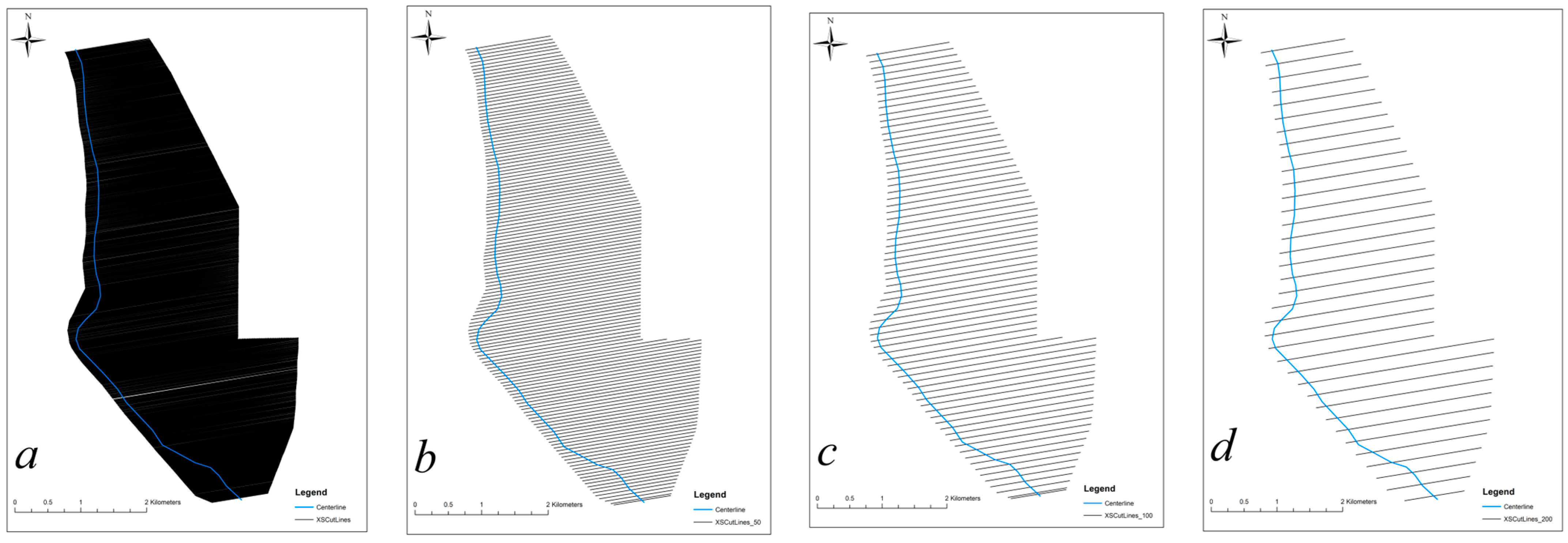
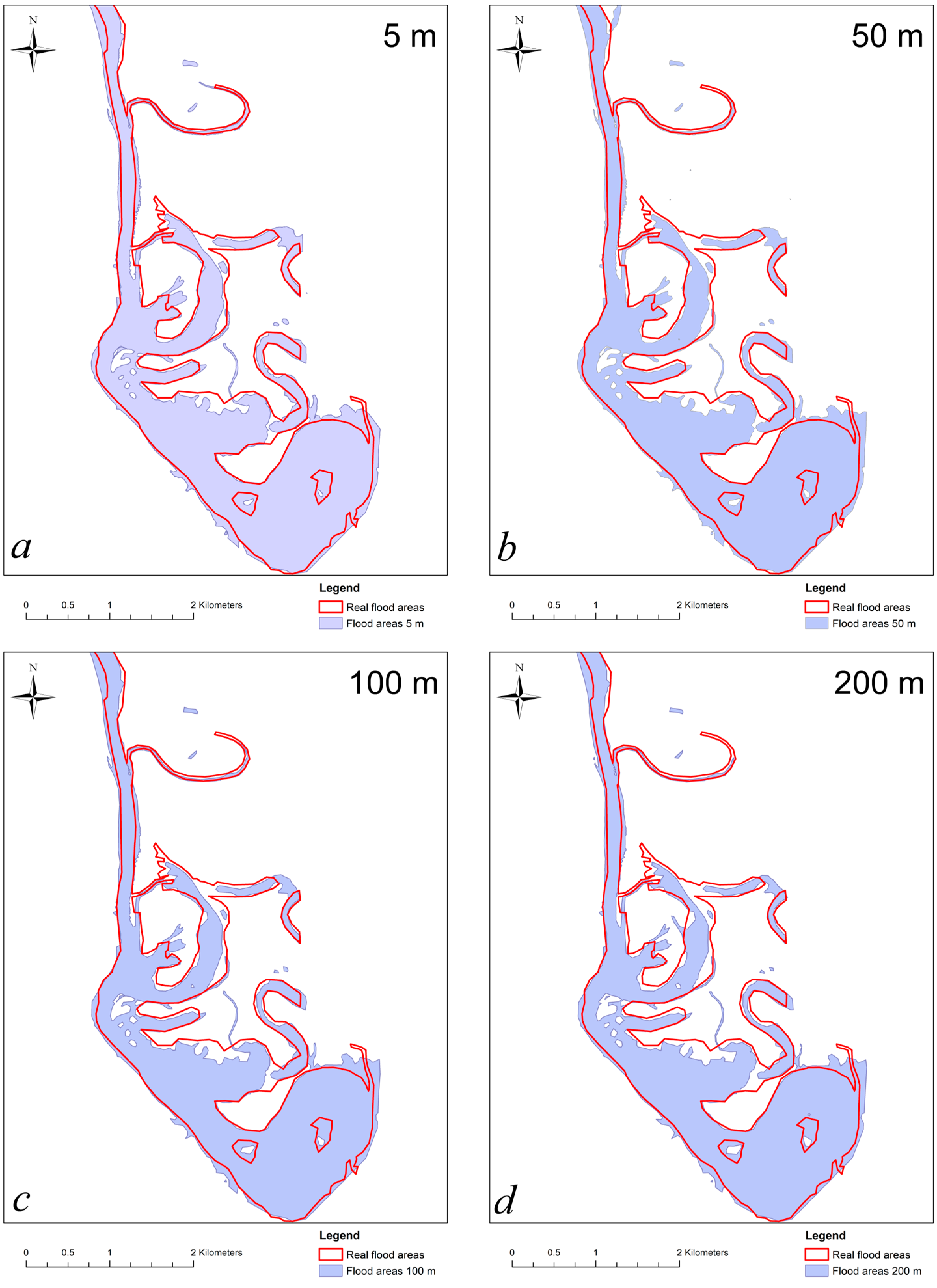
Four values of the intervals between transverse profiles were used to study the effect of the spacing between transverse profiles for the selected site on the modeling accuracy: 5 m, 50 m, 100 m, and 200 m. Figure 7 shows the constructed transverse profiles with different intervals at the study site.

The result of modeling the flooded areas using different intervals between the transverse profiles is shown in Figure 8. The test flood area is circled in red.

The calculated vectorized test area is 600.6 hectares. The areas of the real and modeled flooded sites using different values of the intervals between the transverse profiles are presented in

Table 3. Hydrologic modeling areas using different intervals between transverse profiles.

Spacing between Transverse Profiles (m)	5	50	100	200
Area (ha) 600.6	570.2	558.9	551.4	536.1
Difference, (ha)	30.4	41.7	49.2	64.5
Difference, (%)	5.1	6.9	8.2	10.8

.

The distance between the profiles affects not only the value of the modeling area but also their detail. When large spacing is used, the modeling areas have more generalized shapes, reducing the area value. Figure 9 shows an example of the detail of the modeling results at different intervals of transverse profiles.

Table 3 shows that the accuracy of the modeled flooded area is 5.1% for a 5 m interval, 6.9% for 50 m, 8.2% for 100 m, and 10.8% for 200 m. These results allow determining the degree of influence of the distance between intervals on the modeling accuracy. It is worth noting that when using intervals of 5 m, the area of the modeled site differed least from the test area. This interval size allowed for the most accurate results, but modeling requires much more input information, so for further study, the size between profiles was chosen as 50 m.

3.4. Determination of Manning’s Coefficients for Different Types of Subgrade, Considering Their Changes

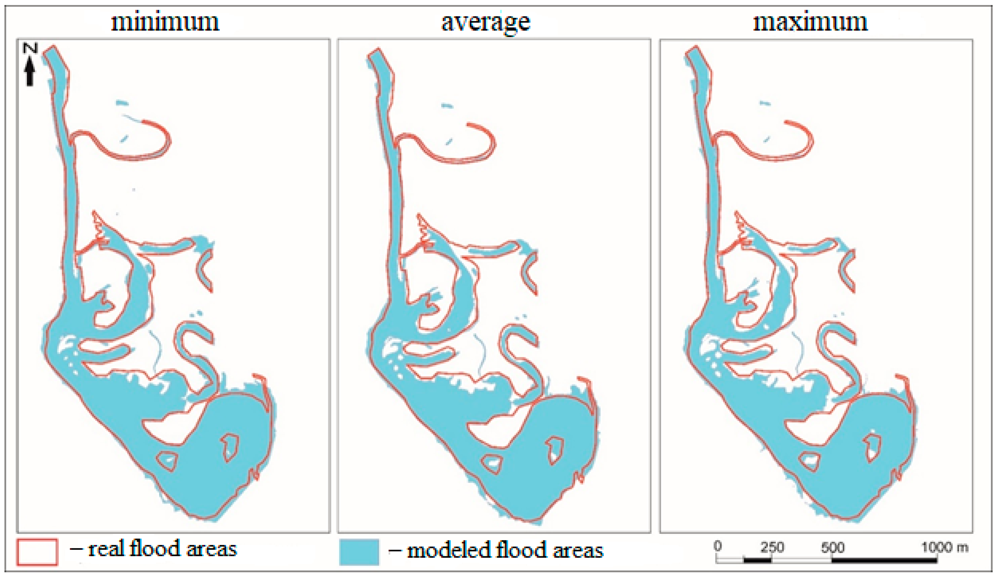
Based on Table 2, which shows the values of Manning’s coefficients for individual sections with different bedding surfaces and the selected spacing between profiles, which was 50 m, the accuracy of the modeling was investigated. After the modeling, the simulated flood areas were obtained in vector form, which allows for determining their areas and comparing them with the test flooded area. The results of the influence of Manning’s coefficients on the modeling result are shown in Figure 10.

The test area is circled in red. The areas of the test and modeled flood areas using the minimum, average, and maximum values of Manning’s coefficients and the calculated differences in regions between the real and modeled data are presented in

Table 4. Areas of actual and modeled flooded areas depending on selected Manning’s coefficients (M).

Test Area	M Minimum	M Average	M Maximum
Area (ha) 600.6	569.2	558.9	541.8
Difference, (ha)	31.4	41.7	58.8
Difference, (%)	5.2	6.9	9.8

.

Table 4 shows that the difference in flooded areas using the limit values of Manning’s coefficient can vary within 5%. The flooded areas obtained using the minimum value of Manning’s coefficient are more significant than those obtained using the maximum value of the coefficient. This is because, with a low roughness of the underlying surface, larger areas will be flooded due to less resistance to flow. The results show that Manning’s coefficients significantly impact modeling accuracy.

4. Conclusions

The paper discusses the theoretical foundations of hydrological modeling and the use of various data to determine the area of flooded land. Based on certain techniques, a methodological approach to hydrological modeling of flooded land zones for the Dniester River channel section is proposed.

Considering the analysis of the main hydrological and morphometric characteristics of the flat section of the riverbed, it is proposed to use a one-dimensional physical model for the hydrological modeling of flooded lands.

The methodology for hydrological modeling of the Dniester River’s plain part with complex relief microforms was developed. The modeling is based on the following procedures: creating high-accuracy DTMs, determining Manning’s coefficients, and determining changes in water level based on a plot obtained from observations at hydrometeorological stations.

A methodology for determining Manning’s coefficients is developed and proposed, considering changes in the bedding surface along the profiles, which are calculated based on remote sensing data. The results of the study can be used to analyze riverbed processes, more accurately identify potentially dangerous areas that could be flooded, identify the most suitable locations for protective structures, and monitor coastal areas.

For the selected sites, the model was parameterized to determine the optimal distance between the transverse profiles and Manning’s coefficients. To assess the accuracy of the hydrological modeling, a high-resolution satellite image was used for the duration of the flood, as of 25 June 2020. The modeling accuracy is about 5% of the flooded area determined from the satellite image. The test area of 600.6 hectares was determined with an accuracy of 0.8%.

The limitations of the study relate to the type of terrain and the characteristics of the flood. For other areas, the methodology is the same, but there may be different modeling parameters.