Multivariate Drought Risk Analysis for the Weihe River: Comparison between Parametric and Nonparametric Copula Methods

Abstract

This study analyzed the multivariate drought risks for the Wei River basin by characterizing the interdependence between the standardized precipitation index (SPI) and the standardized precipitation evapotranspiration index (SPEI). Both parametric and nonparametric copulas were adopted to quantify the dependence between the SPI and SPEI. The results indicated that the Gaussian copula demonstrated the best fit in most cases, while the nonparametric copula method showed superiority over the parametric models at only one out of eighteen meteorological stations. The joint return periods (T^OR, T^AND, and T^Kendall) were computed through copula modeling, providing valuable insights into the co-occurrence of extreme drought events. For the SPI and SPEI with a 50-year return period, the T^OR values range from 25.5 to 37.9 years, the T^AND values fluctuate between 73.4 and 1233 years, and the T^Kendall values range from 60.61 to 574.71 years, indicating a high correlation between the SPI and SPEI in the study area. The spatial analysis revealed varying patterns across the basin with some regions more prone to experiencing simultaneous drought conditions characterized by both the SPI and SPEI. Furthermore, our results indicated that the SPEI exhibited more severity in drought characterization than the SPI due to its consideration of temperature effects. The disparities in the spatial features of the SPI and SPEI underscore the importance of incorporating multiple meteorological factors for a comprehensive drought risk analysis. This research contributes to a better understanding of the drought patterns and their joint risks in the Wei River basin, offering valuable information for drought preparedness and water resource management.

1. Introduction

Drought is a natural disaster that poses significant challenges to societies, economies, and ecosystems worldwide. In recent years, the increasing frequency and severity of drought events have raised concerns among researchers and policymakers [1,2]. Monitoring and assessing drought risk are crucial for the development of effective mitigation and adaptation strategies. The standardized precipitation index (SPI) and standardized precipitation evapotranspiration index (SPEI) are two widely used drought indices in the fields of hydrology and meteorology [3,4]. The SPI characterizes meteorological drought by measuring the deviation of precipitation from its long-term average, while the SPEI incorporates both precipitation and potential evapotranspiration, offering a comprehensive view of hydrological drought [4,5]. These indices have been proven valuable for drought monitoring and early warning systems, enabling decision-makers to implement timely measures to alleviate the impacts of drought [6,7,8,9]. However, assessing drought risk based solely on individual indices may not provide a complete understanding of the complex interactions and dependencies between meteorological and hydrological drought events. This limitation calls for a more integrated approach that considers the joint behavior of the SPI and SPEI to provide a more comprehensive characterization of drought risk [10].

Copula analysis has emerged as a powerful tool in the fields of hydrology and drought risk assessment, allowing researchers to model the joint behavior of multiple variables accurately. The application of copulas in hydrology dates back to the early 1990s, but it has gained significant traction in recent years due to its ability to capture the complex dependencies between hydrological processes and climatic variables [11,12]. Copula-based methods have proven valuable in analyzing extreme events, providing a more comprehensive understanding of droughts and their interactions with other hydroclimatic variables. In the context of drought risk assessment, copulas have been applied to investigate the joint behavior of various drought indices, such as the SPI and SPEI, and other relevant hydroclimatic variables. Wang et al. [13] used a new copula-based standardized precipitation evapotranspiration streamflow index (SPESI) to characterize meteorological and hydrological drought in the Yellow River basin. Their findings highlighted the potential benefits of considering the joint probabilities of drought events, leading to more effective drought management strategies. Copula-based approaches have also been employed in the estimation of drought return periods and frequency analysis, providing valuable insights into the long-term behavior of drought events [14,15]. Additionally, copula methods have been used to explore the dependence structure of other correlated variables, such as compound flood risks, climate downscaling, and so on [16,17,18]. The flexibility of copulas allows researchers to select suitable copula families based on the data characteristics and research objectives. Archimedean copulas, such as the Clayton, Gumbel, and Frank copulas, are commonly used in drought risk analysis due to their simplicity and ability to model tail dependencies [19]. In addition to Archimedean copulas, Gaussian copulas have also been widely applied in multivariate modeling of environmental variables and provide greater flexibility in capturing complex, non-monotonic relationships between variables [20,21].

Despite its many advantages, copula analysis in drought risk assessment faces certain challenges and limitations. The selection of an appropriate copula function and the determination of the optimal parameters can be sensitive to the dataset and require careful consideration [19]. Recently, nonparametric copula methods have been proposed for coastal flood risk analysis to avoid misspecification issues associated with parametric copula models [22,23]. These studies have demonstrated the applicability of nonparametric copula methods in capturing the interdependence among flood variables. However, the demonstration of nonparametric copula methods for drought risk analysis remains limited, and there is a lack of performance comparison between parametric and nonparametric copulas for multivariate drought risk inference.

Consequently, the objective of this study is to compare the performances of both parametric and nonparametric copulas on multivariate drought risk analysis for the Wei River basin. The drought events will be characterized by the SPI and SPEI values based on monthly rainfall and temperature observations. The annual minimum SPEI and the corresponding SPI would be further identified to reflect the most severe drought event in each year. The interdependence between the SPI and SPEI will be modeled using both parametric and nonparametric copulas, and their performances will be evaluated based on goodness-of-fit measures, such as the Akaike information criterion (AIC). Here, the AIC would be used to identify the most appropriate marginal and copula models since this method is able to evaluate the fitting effect of different distributions and penalize the model with more parameters. The best copula models will then be employed to reveal the joint risks of compound droughts, as reflected by the SPI and SPEI, for the Wei River basin.

This comparative analysis of copula methods for drought risk assessment will contribute to the existing literature by shedding light on the suitability of both parametric and nonparametric approaches for modeling drought dependencies. The findings of this study will provide valuable insights for drought management and decision-making in the Wei River basin and other regions facing similar hydroclimatic challenges.

2. Methodology

2.1. Copula Method

Copula analysis is a powerful statistical technique used to model the dependence structure between multivariate random variables while preserving their individual marginal distributions. Consider d correlated random variables X₁, X₂, …, X_d with their marginals denoted as F₁, …, F_d, their joint cumulative distribution function (CDF) F(.) can be constructed through a copula function as follows [24]:

$$F\left(x_1,x_2,\dots ,x_d\right)=C\left(F_1\left(x_1\right), F_2\left(x_2\right),\dots ,F_d\left(x_d\right)\right)$$

(1)

where C(.) is the copula function, which is unique if F_i (i = 1, 2, …, d) is continuous. The multivariate probability density function (PDF) f(.) would also be formulated as follows [25]:

$$f\left(x_1,x_2,\dots ,x_d\right)=c\left(u_1,u_2,\dots ,u_d\right){\prod }_{i=1}^d{f}_i\left(x_i\right)$$

(2)

where $c\left(u_1,u_2,\dots ,u_d\right)$ is the copula density function, and u_i = F_i(x_i). $f_i\left(x_i\right)$ is the marginal PDF for random variable X_i.

2.2. Parametric Copulas

The Archimedean copulas are a class of copulas that are commonly used due to their simplicity and tractability. A bivariate Archimedean copula is defined as follows [26]:

$$C\left(u_1,u_2|\theta \right)={\phi }^{-1}(\phi \left(u_1\right)+\phi (u_2\left)\right)$$

(3)

where φ is the copula generator that is a convex decreasing function with φ(1) = 0 and φ⁻¹(.) = 0 when u₂ ≥ φ(0); θ is the parameter hidden in the generating function [26]. The most commonly used Archimedean copulas include the Clayton, Gumbel, and Frank copulas.

In addition to the Archimedean copulas, the Gaussian copula is also commonly used when dealing with continuous variables. The joint CDF of the Gaussian copula is given as follows:

$$C\left(u_1,u_2|\mathsf{\Sigma }\right)=\mathsf{\Phi }({\mathsf{\Phi }}^{-1}\left(u_1\right),{\mathsf{\Phi }}^{-1}\left(u_2\right)|\mathsf{\Sigma })$$

(4)

where Φ denotes the multivariate Gaussian CDF with correlation matrix Σ, and Φ⁻¹ is the inverse standard Gaussian CDF.

Table 1. Basic properties of parametric copulas.

Copula Name	Function [C(u1, u2)]	Parameter Range	$\mathbf{Generator} \mathbf{Functions} [\mathit{\phi }(\mathit{t})]$
Gaussian	$\mathsf{\Phi }({\mathsf{\Phi }}^{-1}\left(u_1\right),{\mathsf{\Phi }}^{-1}\left(u_2\right)|\mathsf{\Sigma })$	$\mathsf{\Sigma }\in (-1,1)$
Joe	$1-[{\left(1-u_1\right)}^{\theta }+{\left(1-u_2\right)}^{\theta }$ $-{\left(1-u_1\right)}^{\theta }{\left(1-u_2\right)}^{\theta }{]}^{1/\theta }$	$\mathsf{\theta }\in [1,\mathrm{\infty })$	$-\mathrm{l}\mathrm{n}(1-{\left(1-t\right)}^{\theta })$
Gumbel	$\mathrm{e}\mathrm{x}\mathrm{p}\{-{[{(-\mathrm{l}\mathrm{n}{(u}_1))}^{\theta }+{(-\mathrm{l}\mathrm{n}{(u}_2)}^{\theta }]}^{1/\theta }\}$	$\mathsf{\theta }\in [1,\mathrm{\infty })$	$-\mathrm{l}\mathrm{n}(t^{\theta })$
Frank	$-\frac{1}{\theta }\mathrm{l}\mathrm{n}\{1+\frac{(e^{-\theta u_1}-1)(e^{-\theta u_2}-1)}{e^{-\theta }-1}\}$	$\mathsf{\theta }\in [-\mathrm{\infty },\mathrm{\infty })\backslash \{0\}$	$-\mathrm{l}\mathrm{n}[\frac{e^{-\theta t}-1}{e^{-\theta }-1}]$

presents the formulations for the Gaussian, Frank, Gumbel, and Joe copulas as well as their basic properties. All the copulas are characterized by specific mathematical functions with a fixed number of parameters. These copulas assume a predefined functional form, which simplifies the modeling process and parameter estimation. In parametric copula modeling, the selection of the appropriate copula function and the estimation of its parameters play a crucial role in accurately capturing the dependence structure between variables. Even though there is a large variety of parametric copula models, they notoriously lack flexibility and bear the risk of misspecification [27].

2.3. Nonparametric Copulas

A specific class of nonparametric density estimators are kernel estimators, which have been applied for exploratory data analysis and widely used in many disciplines [27,28]. Consider n observations (U_i1, U_i2), i = 1, …, n, from a bivariate copula C, the corresponding density function c(u₁, u₂) can be estimated through the kernel density estimator as follows [27]:

$${\widehat{c}}_n\left(u_1,u_2\right)=\frac{1}{n}{\sum }_{i=1}^n{K}_{b_n}(u_1-U_{i1})K_{b_n}\left(u_2-U_{i2}\right), (u_1, u_2)\in {[0, 1]}^2$$

(5)

where the notation K_b(·) = K(·/b)/b. The kernel function K is typically a symmetric, bounded probability density function on R², and b_n > 0 is the smoothing or bandwidth parameter. The estimator in Equation (5) will result in a considerable amount of probability mass outside the unit square, leading to ${\widehat{c}}_n\left(u_1,u_2\right)$ not being a valid density function on [0, 1]² due to its integral not equaling one [27]. Furthermore, the estimator will also suffer from severe bias at the boundaries [27]. Some approaches have been developed to tackle the above challenges, including the mirror-reflection method, the beta kernel method, and the transformation method [29,30]. The kernel density estimator allows us to estimate the bivariate copula density function nonparametrically, avoiding the need to assume a specific functional form and providing a flexible approach to capture the underlying dependence structure of the data.

2.4. Primary and Secondary Return Periods

If appropriate copula functions are selected to capture the joint probabilistic characteristics among correlated extreme variables, it becomes possible to derive conditional, primary, and secondary return periods. Specifically, joint (primary) return periods, referred to as “OR” and “AND” return periods, can be formulated as follows [26,31,32,33]:

$$T_{}^{OR}=\frac{\mu }{1-C(u_1,u_2)}$$

(6)

$$T_{}^{AND}=\frac{\mu }{1-u_1-u_2+C(u_1,u_2)}$$

(7)

where μ is the mean inter-arrival time of the two consecutive extreme events. Additionally, the secondary return period, referred to as the Kendall’s return period, is defined as follows [26,31,32,33]:

$$\overline{T}=\frac{\mu }{1-K_C\left(t\right)}$$

(8)

where K_C is Kendall’s distribution associated with the theoretical Copula function C(.). For the Archimedean copulas, K_C can be expressed as follows [26,31,32,33]:

$$K_C\left(t\right)=t-\frac{\phi \left(t\right)}{{\phi }^{\prime }\left(t^{+}\right)}$$

(9)

where ${\phi }^{\prime }\left(t^{+}\right)$ is the right derivative of the copula generator function $\phi \left(t\right)$.

3. Case Study

3.1. Overview of Wei River Basin

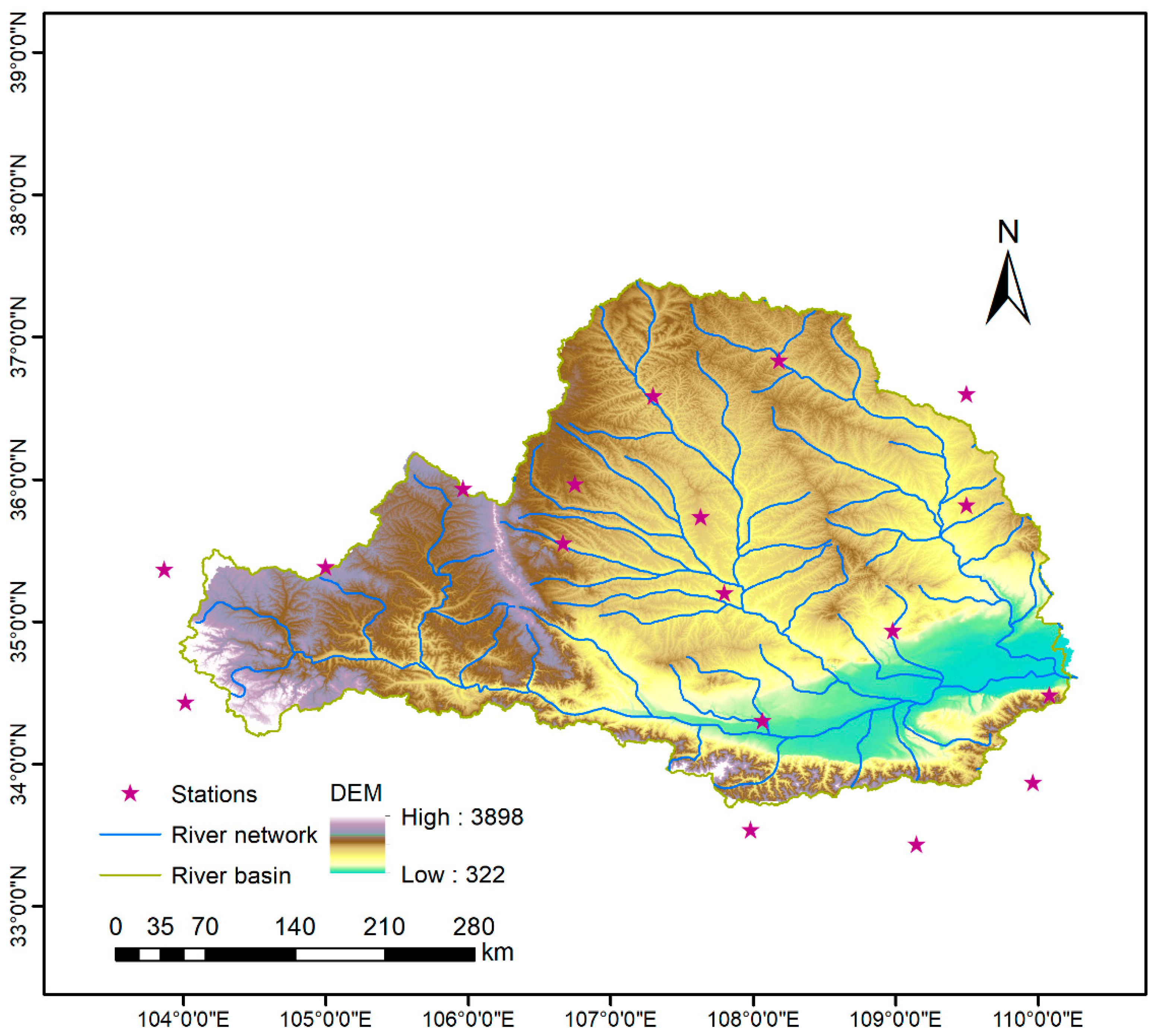
The Wei River basin, as shown in Figure 1, is one of the major river basins in China, encompassing an extensive area in the central and northwest regions. It is a crucial water resource for both agricultural and industrial activities in the region. The basin is characterized by a semi-arid to arid climate, experiencing irregular precipitation patterns with considerable variations in both temporal and spatial distributions. This region is prone to drought events due to its climate characteristics and limited water resources. Droughts in the region can have severe impacts on agriculture, water supply, and the ecosystem, posing significant challenges for water resource management and drought risk assessment [34]. Over the past few decades, the Wei River basin has experienced varying degrees of drought severity, ranging from mild to severe drought events [35]. These drought occurrences have highlighted the need for effective drought risk assessment and management strategies to mitigate the socio-economic and environmental impacts of drought in the region.

3.2. Data Collection and Drought Identification

The historical rainfall and temperature data between 1971 and 2016 were collected from the China Meteorological Data Service Center (http://data.cma.cn/en, accessed on 30 September 2022). The monthly rainfall and temperature data from a total of 18 meteorological stations located around the Wei River basin were utilized in this study for drought risk inference. The geographical positions of these stations are indicated in Figure 1 with the detailed locations and elevations presented in

Table 2. Meteorological station information.

ID	Lat (°C)	Lon (°C)	Elevation (m)
52986	35.36667	103.8667	1886.6
52996	35.38333	105	2450.6
53738	36.83333	108.1833	1272.6
53817	35.96667	106.75	1753.2
53821	36.58333	107.3	1255.6
53845	36.6	109.5	957.6
53903	35.93333	105.9667	1901.3
53915	35.55	106.6667	1346.6
53923	35.73333	107.6333	1421.9
53929	35.2	107.8	1206.3
53942	35.81667	109.5	1158.3
56093	34.43333	104.0167	2314.6
57034	34.3	108.0667	505.4
57037	34.93333	108.9833	719
57046	34.48333	110.0833	2064.9
57134	33.53333	107.9833	1179.2
57144	33.43333	109.15	1098.6
57143	33.86667	109.9667	742.2

.

Both the SPI and SPEI were adopted to characterize the historical drought events. For the SPI, the gamma probability distribution function was used to calculate the probability distribution of the precipitation in a specific month as follows [3,36]:

$$f\left(x\right)=\frac{1}{{\beta }^{\gamma }\Gamma \left(\gamma \right) }{x}^{\gamma -1}{e}^{-x/\beta }, x>0$$

(10a)

$$\Gamma \left(\gamma \right)={\int }_0^{\infty }{x}^{\gamma -1}{e}^{-x}dx$$

(10b)

where β > 0 and γ > 0 are scale and shape parameters, respectively, calculated as follows:

$$\gamma =\frac{1+\sqrt{1+A/3}}{4A}$$

(10c)

$$\beta =\overline{x}/\gamma$$

(10d)

$$A=\ln \overline{x}-\frac{1}{n}{\sum }_{i=1}^n\ln x_i$$

(10e)

where x_i is the monthly precipitation, n refers to the sample size, and $\overline{x}$ is the average of the precipitation samples. The probability of the random variable x less than x₀ can be derived as follows:

$$\mathrm{Pr}\left\{x<x_0\right\}={\int }_0^{x_0}\frac{1}{{\beta }^{\gamma }\Gamma \left(\gamma \right) }{x}^{\gamma -1}{e}^{-x/\beta }dx$$

(11)

The gamma probability distribution in Equation (11) is normalized as follows:

$$\mathrm{Pr}\left\{x<x_0\right\}=\frac{1}{\sqrt{2\pi }}{\int }_0^{x_0}{e}^{-z^2/2}dx$$

(12)

The gamma function does not include the case of x = 0, and the probability distribution with the x = 0 cases would be modified as follows:

$$P\left(x\right)=q+(1-q)F\left(x\right)$$

(13)

where q is the probability for zero precipitation, and F(x) is the probability from the gamma distribution. The SPI can finally be derived as follows [37]:

$$SPI=z=S\frac{c_0+W-c_{1}W-c_2{W}^2}{1+d_{1}W+d_2{W}^2+d_3{W}^3}$$

(14a)

$$W=\sqrt{\frac{1}{H^2}}\left\{\begin{array}{c}P=1-F\left(x\right), S=-1 for F\left(x\right)\le 0.5\\ P=1-P, S=1, for F\left(x\right)>0.5\end{array}\right.$$

(14b)

where the constants are c₀ = 2.515517, c₁ = 0.802853, c₂ = 0.010328, d₁ = 1.432788, d₂ = 0.189269, and d₃ = 0.001308. The Gamma distributions for the monthly precipitation were tested with the Anderson–Darling test with their p-values provided in Table S1. The results suggest that the Gamma distributions can pass the statistical test for most months at each station except that some rejections occurred in December at some stations. However, the Gamma distributions would still be applicable in this study since only the annual minimum SPI values were analyzed, which seldom occurred in December.

The SPI has its limitations since it only considers the precipitation in its calculation process and cannot fully reflect the impact of climate warming on drought [4]. Consequently, the SPEI has been developed based on the monthly water balance to reflect the impact of surface evaporation changes in order to compensate for the lack of the SPI [4,36].

In order to obtain the monthly water balance, the potential evapotranspiration (PET) was first calculated with the Hargreaves model as follows [38,39]:

$$PET=0.0023R_a\left(T_{mean}+17.8\right)\times \sqrt{T_{max}-T_{min}}$$

(15)

where T_mean is the average air temperature (°C); T_max and T_min are the maximum and minimum air temperatures (°C), respectively; and R_a is the daily net radiation on the land surface (MJ m⁻² d⁻¹). The water balance can then be obtained as follows:

D_i = P_i − PET_i

(16)

where D_i, P_i, and PET_i respectively denote the water balance, monthly precipitation, and monthly potential evapotranspiration. In this study, the GEV distribution was employed to normalize the water balance series (i.e., D_i) with the density function expressed as follows [38]:

$$f\left(x\right)=\left\{\begin{array}{c}\frac{1}{\sigma }{\left[{\left(1+\xi z\left(x\right)\right)}^{-\frac{1}{\xi }}\right]}^{(\xi +1)}·e^{-{[\left(1+\xi z\left(x\right)\right)}^{-\frac{1}{\xi }}]}, \xi \ne 0, 1+\xi z\left(x\right)>0\\ \left(\frac{1}{\sigma }\right)e^{-z\left(x\right)-e^{-z\left(x\right)}}, \xi =0,-\infty <x<\infty \end{array}\right.$$

(17)

where z(x) = (x − μ)/σ; ξ, σ, and µ are the shape, scale, and location parameters, respectively. Based on the cumulative distribution function F(x) of GEV, the SPEI can be easily standardized as follows [38]:

$$SPEI=W-\frac{c_0+c_{1}W+c_2{W}^2}{1+d_{1}W+d_2{W}^2+d_3{W}^3}$$

(18)

where W = $\sqrt{-2\mathrm{l}\mathrm{n}\left(P\right)}$ for P ≤ 0.5, and P = 1 − F(x). If P > 0.5, then P is replaced with 1 − P, and the sign of the resultant SPEI is reversed. The constants are c₀ = 2.515517, c₁ = 0.802853, c₂ = 0.010328, d₁ = 1.432788, d₂ = 0.189269, and d₃ = 0.001308. The GEV distributions were tested with the Anderson–Darling test with their p-values provided in Table S2 [40]. The results suggest that the GEV distributions can pass the statistical test for all months at each station, indicating its applicability to derive the SPEI values.

4. Results Analysis

4.1. Probability Estimation of Individual Drought Index

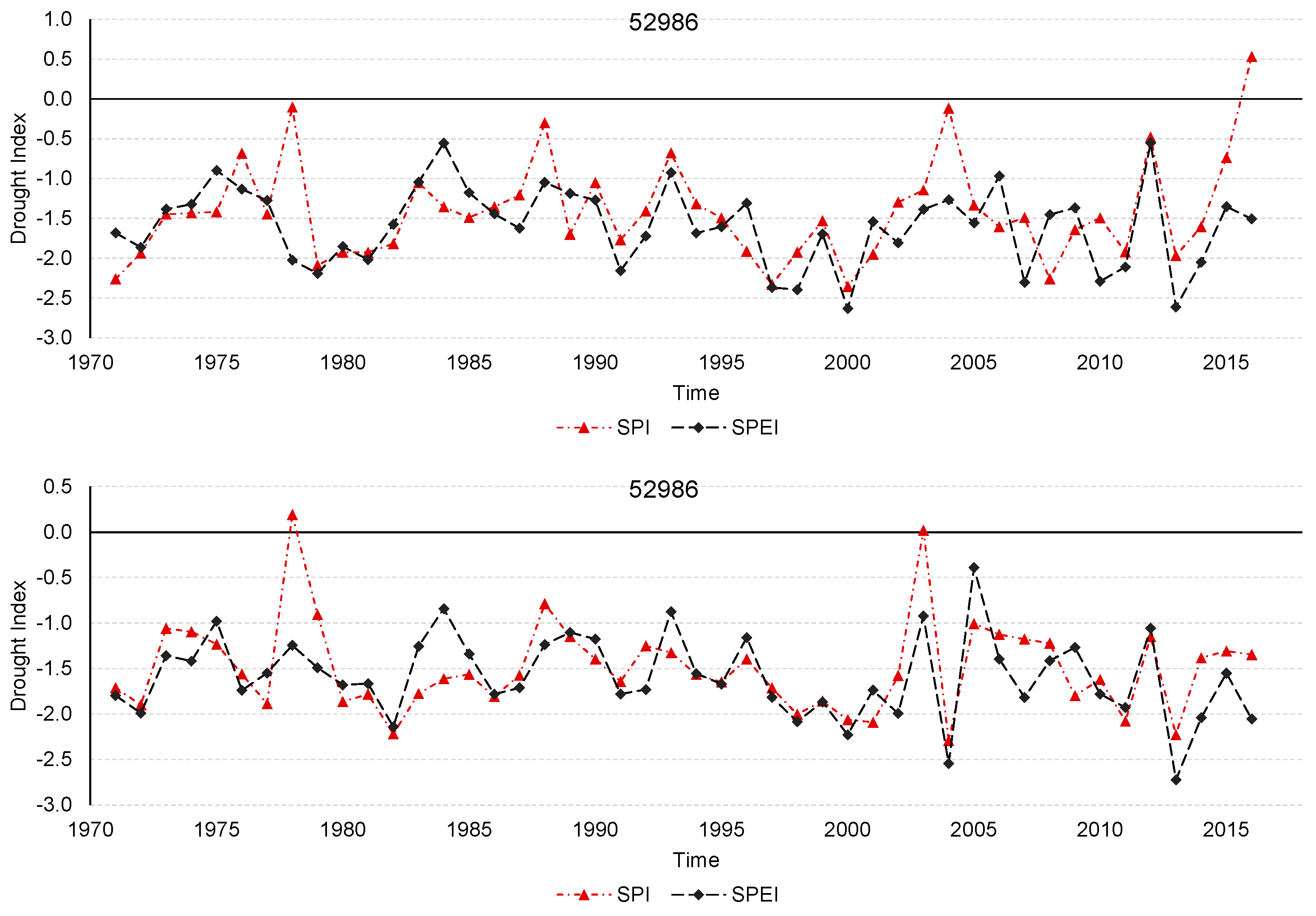
Figure 2 presents the general procedures to derive the SPI and SPEI values and then predict the multivariate drought risks. In this study, the one-month SPI and SPEI values were derived respectively from the Gamma and GEV distributions. The annual minimum SPEI values as well as the corresponding SPI values were identified for the period of 1971–2016.

Table 3. Basic statistics of the SPI and SPEI values and their correlations at different stations.

Station ID	SPI		SPEI		Kendall between SPI and SPEI
	Mean	Sd	Mean	Sd
52986	−1.419	0.624	−1.592	0.505	0.386
52996	−1.490	0.505	−1.584	0.455	0.472
53738	−1.384	0.818	−1.657	0.527	0.317
53817	−1.412	0.568	−1.677	0.489	0.291
53821	−1.355	0.660	−1.603	0.563	0.535
53845	−1.377	0.595	−1.590	0.554	0.403
53903	−1.371	0.643	−1.620	0.524	0.369
53915	−1.402	0.524	−1.611	0.507	0.432
53923	−1.445	0.422	−1.551	0.512	0.555
53929	−1.411	0.532	−1.548	0.496	0.435
53942	−1.538	0.505	−1.622	0.583	0.584
56093	−1.309	0.756	−1.592	0.589	0.527
57034	−1.475	0.465	−1.577	0.467	0.483
57037	−1.568	0.449	−1.574	0.495	0.370
57046	−1.486	0.454	−1.546	0.462	0.698
57134	−1.427	0.485	−1.629	0.384	0.391
57144	−1.446	0.539	−1.546	0.537	0.418
57143	−1.500	0.468	−1.601	0.514	0.515

presents some basic statistics of the SPI and SPEI values as well as their Kendall correlations at the different stations. The results suggest that the droughts respectively characterized by the SPI and SPEI are highly correlated, which raised the requirement to reveal the interdependence between these two kinds of drought. Figure 3 presents the temporal variations in the SPI and SPEI at stations 52986 and 52996, which also indicate the correlation between these two drought indicators.

One of the major advantages of copula methods for multivariate drought risk analysis is that they allow for the quantification of marginal distributions of individual variables and their dependence structures in separate processes. In this study, multiple distribution methods were employed to quantify the random features of the annual minimum SPEI and SPI values. The goal was to identify the most appropriate distribution models for these two indices at different stations.

In detail, five distributions, namely the Gumbel, generalized extreme value (GEV), Gamma, lognormal, and Weibull distributions, were employed to quantify the distribution features of the SPI and SPEI. The performance of each distribution model was further evaluated using both the Kolmogorov–Smirnov (KS) test and the Akaike information criterion (AIC) to identify the most appropriate distributions for the SPI and SPEI. The KS test was used to assess how well each distribution fits the empirical data, while the AIC provided a measure to balance goodness-of-fit and model complexity, aiding in the selection of the best-fitting distributions for the drought indices.

Table 4. Selection of marginal distribution at different stations.

Station ID	SPI			SPEI
	Distribution	p-Value (KS)	AIC	Distribution	p-Value (KS)	AIC
52986	GEV	0.9948	−278.27	Gamma	1.0000	−336.81
52996	GEV	0.9942	−310.82	Weibull	0.9944	−305.30
53738	GEV	0.9933	−278.37	Weibull	0.9936	−291.65
53817	GEV	0.9959	−288.31	Gumbel	1.0000	−363.26
53821	GEV	0.9942	−319.34	GEV	1.0000	−327.56
53845	GEV	0.9950	−304.78	GEV	1.0000	−327.82
53903	GEV	0.9942	−301.65	Weibull	0.9944	−293.43
53915	Weibull	1.0000	−348.92	GEV	1.0000	−342.69
53923	Weibull	1.0000	−305.77	GEV	0.9952	−309.03
53929	GEV	0.9479	−293.35	GEV	0.9952	−319.24
53942	GEV	0.9950	−311.08	GEV	1.0000	−357.52
56093	GEV	0.9933	−268.81	GEV	0.9377	−267.38
57034	GEV	1.0000	−345.67	GEV	0.9959	−306.45
57037	GEV	0.9493	−282.44	GEV	0.9523	−301.61
57046	Weibull	0.9513	−299.15	GEV	1.0000	−339.08
57134	GEV	1.0000	−331.43	GEV	0.9959	−324.45
57144	GEV	0.9468	−270.23	GEV	1.0000	−337.80
57143	GEV	1.0000	−333.67	GEV	1.0000	−347.42

presents the marginal distribution selections for the SPI and SPEI at various stations within the Wei River basin. For the SPI, the generalized extreme value (GEV) distribution was predominantly identified as the most suitable model, which presented the lowest AIC values among the five candidate distributions for most stations. Also, the p-values from the KS test are all larger than 0.05, showing the statistical applicability of the selected GEV models. Additionally, the Weibull distribution was chosen for three stations due to the lowest AIC values and high p-values at these stations. Similarly, for the SPEI, the GEV distribution was the primary choice, being deemed most appropriate for 13 out of the 18 stations. The Weibull distribution was the second option, considered suitable for three stations, while the choices for the remaining two stations were the Gamma and Gumbel distributions, respectively.

Overall, the findings demonstrate that the GEV distribution serves as a robust choice for characterizing the marginal distributions of both the SPI and SPEI across the Wei River basin. However, it is evident that certain stations exhibited slight variations in their optimal distribution models, highlighting the spatial variability in drought characteristics within the basin.

4.2. Quantification of Interdependence between SPI and SPEI through Both Parametric and Nonparametric Copulas

As presented in Table 3, the SPI and SPEI are highly correlated with their Kendall’s correlation larger than 0.3 for most stations and highest correlation approaching 0.7. In order to quantify the interdependence between the SPI and SPEI, both parametric copula models, as listed in Table 1, and nonparametric copula models were utilized. Similar to the selection process of marginal distributions, we employed the Kolmogorov–Smirnov (KS) test and the Akaike information criterion (AIC) to identify the most appropriate copula model at each station. For the nonparametric copula models, we calculated the effective number of parameters using the R package “kdecopula” [27], which helped us compute the AIC values for these models. Additionally, we used the root-mean-square error (RMSE) as an additional metric to evaluate the performance of the different copula models.

Table 5. Performances of the best parametric copula and nonparametric copula at each station.

Station ID	Parametric Copula				Nonparametric Copula
	Option	p-Value (KS)	RMSE	AIC	p-Value (KS)	RMSE	AIC
52986	Gumbel	0.9357	0.0316	−309.03	0.9395	0.0322	−290.72
52996	Gumbel	0.8041	0.0281	−312.21	0.9999	0.0255	−292.88
53738	Gaussian	0.9903	0.0333	−290.58	0.9901	0.0341	−271.71
53817	Gaussian	0.9942	0.0348	−306.83	0.9945	0.0282	−310.41
53821	Frank	0.9925	0.0268	−316.37	0.9920	0.0263	−302.81
53845	Gaussian	0.9373	0.0296	−314.85	0.9389	0.0284	−303.40
53903	Gaussian	0.9999	0.0244	−324.92	0.9928	0.0261	−302.56
53915	Frank	0.9921	0.0227	−338.76	0.9414	0.0210	−326.53
53923	Gaussian	0.9401	0.0275	−321.57	0.9401	0.0276	−305.10
53929	Gaussian	0.9999	0.0338	−302.91	0.9389	0.0316	−292.81
53942	Gumbel	0.9935	0.0219	−341.91	0.9939	0.0318	−304.00
56093	Gumbel	0.9295	0.0415	−271.63	0.9910	0.0491	−253.37
57034	Joe	1.0000	0.0227	−346.27	1.0000	0.0255	−321.08
57037	Joe	0.8196	0.0271	−330.07	0.6459	0.0356	−302.80
57046	Joe	0.9947	0.0247	−338.62	0.9424	0.0257	−317.68
57134	Frank	0.8116	0.0274	−329.08	0.9441	0.0241	−326.43
57144	Joe	0.9936	0.0315	−309.24	0.9933	0.0442	−275.99
57143	Gumbel	1.0000	0.0292	−323.20	1.0000	0.0259	−318.21

presents the performance of both the best parametric copula and nonparametric copula models at different stations in the Wei River basin for multivariate drought risk analysis. The parametric copulas include the Gaussian, Gumbel, Frank, and Joe copulas, as shown in Table 1, in which the best parametric copulas with the lowest AIC values are presented in Table 5. In comparison, the nonparametric copula is expressed in Equation (5), and its performances at all stations are presented in Table 5.

The performance of the parametric copula models varied across the stations with different copula functions showing better fits in different cases. In general, the Gaussian copula was primarily selected, being deemed most appropriate for six out of the eighteen stations, followed by the Gumbel, Joe, and Frank copulas.

Regarding the nonparametric copula methods, they demonstrated competitive performance compared to the parametric models. However, it is important to note that the nonparametric model does not necessarily outperform the parametric copulas in quantifying the interdependence between the SPI and SPEI in the Wei River basin. Specifically, the nonparametric copula generated lower RMSE values at eight out of eighteen stations. Nevertheless, due to the inclusion of more effective parameters in the nonparametric copula, this model showed the least AIC value only at Station 53817. In other words, the nonparametric copula exhibited the best performance at only one station in this area.

4.3. Primary and Joint Return Period of SPI and SPEI

Table 6. SPI and SPEI values with a 50-year RP and their corresponding joint return periods.

Station ID	SPI	SPEI	TOR (Year)	TAND (Year)	TKendall (Year)
52986	−2.30	−2.86	33.18	101.43	78.62
52996	−2.35	−2.48	34.30	92.21	76.22
53738	−2.64	−2.68	28.54	201.35	120.48
53817	−2.25	−3.00	26.88	357.73	170.65
53821	−2.15	−2.89	26.97	341.57	187.97
53845	−2.35	−2.77	28.50	203.35	121.07
53903	−2.40	−2.70	27.63	262.44	173.61
53915	−2.32	−2.66	26.18	555.44	264.55
53923	−2.14	−2.60	30.46	139.40	97.28
53929	−2.31	−2.48	29.16	175.15	126.26
53942	−2.31	−2.78	37.33	75.67	67.84
56093	−2.29	−2.58	36.99	77.14	62.58
57034	−2.61	−2.69	25.68	948.29	458.72
57037	−2.21	−2.52	25.52	1233.03	574.71
57046	−2.39	−2.55	26.31	501.76	273.22
57134	−2.35	−2.56	25.99	656.36	362.32
57144	−2.34	−2.57	37.92	73.39	60.61
57143	−2.45	−2.53	27.92	238.92	147.93

presents the SPI and SPEI values with a 50-year return period (RP) and their corresponding joint return periods across the Wei River basin. Here, the 50-year return period is considered since (i) this RP would generally show severe drought events, and (ii) this RP has been analyzed in most drought research studies. Drought events with other RPs can be similarly generated with the proposed modelling method.

The analysis of the results reveals the severity of drought conditions in the region based on the SPI and SPEI values with a 50-year RP at various meteorological stations. The SPI values range from −2.14 to −2.64, while the SPEI values vary from −2.48 to −3.00, indicating the presence of significant and prolonged drought conditions across the basin.

Furthermore, the joint return periods, including T^OR, T^AND, and T^Kendall, obtained through copula modeling provide valuable insights into the co-occurrence of extreme drought events. T^OR represents the time of occurrence for droughts when either the SPI or SPEI falls below their respective 50-year RP thresholds. As shown in Equation (6), u₁ = u₂ = 0.98 since both the SPI and SPEI have an RP of 50 years. T^OR can then be derived from the obtained copula model based on Equation (6). For instance, at station 52986, the Gumbel copula was selected; thus, we can have T^OR = $1/[1-\mathrm{e}\mathrm{x}\mathrm{p} \{-{[{(-\mathrm{l}\mathrm{n}{(u}_1))}^{\theta }+{(-\mathrm{l}\mathrm{n}{(u}_2)}^{\theta }]}^{1/\theta }\}]$ = 33.18 years, where u₁ = u₂ = 0.98 and θ = 1.669, obtained in Section 4.2. In summary, the T^OR values range from 25.5 to 37.9 years, indicating the timing of individual drought events below the SPI or SPEI with a 50-year RP. On the other hand, the T^AND values fluctuate between 73.4 and 1233 years, representing the time of occurrence for droughts when both the SPI and SPEI are simultaneously below their 50-year RP thresholds.

Additionally, the T^Kendall values, ranging from 60.61 to 574.71, indicate the likelihood of compound drought occurrences where both the SPI and SPEI experience extreme droughts simultaneously. These joint return periods emphasize the importance of considering the interdependence between the SPI and SPEI for a comprehensive understanding of drought risks in the Wei River basin.

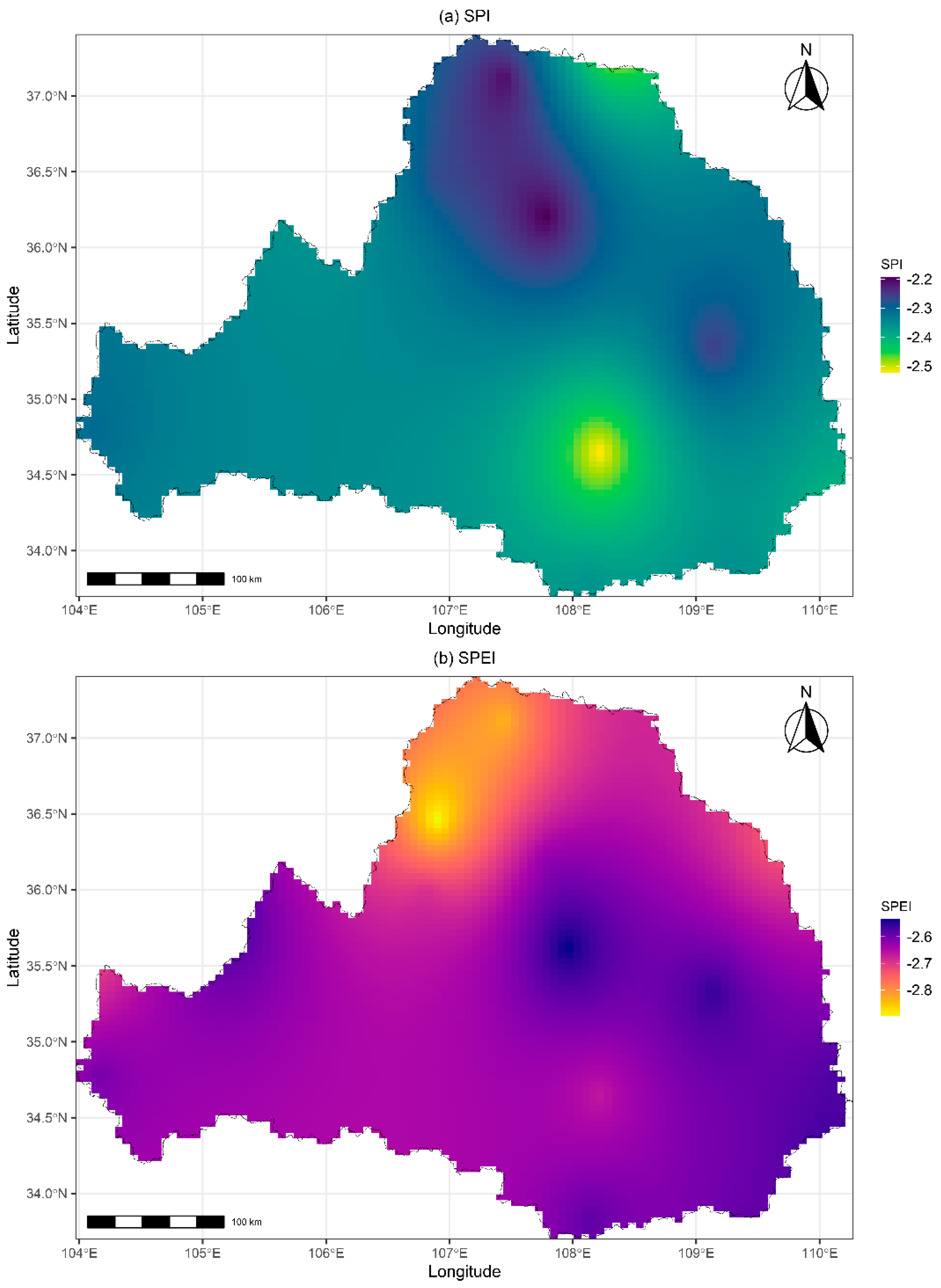
Figure 4 illustrates the spatial variations of the SPI and SPEI values with a 50-year RP in the Wei River basin, which were interpolated with the Kriging method based on station results. The results indicate that the SPEI appears to show more severity than the SPI as it takes into account the influence of temperature on drought conditions in addition to precipitation. Moreover, the SPI and SPEI exhibit different spatial features across the basin. In particular, the northwest region experiences the most severe droughts according to the SPEI, while the SPI identifies relatively milder drought severity in this area. Conversely, the central-south area exhibits the most severe droughts according to the SPI with drought severity characterized by the SPEI ranging between −2.6 and −2.7, approaching the least drought severity regions (i.e., central and southeast) as identified by the SPEI.

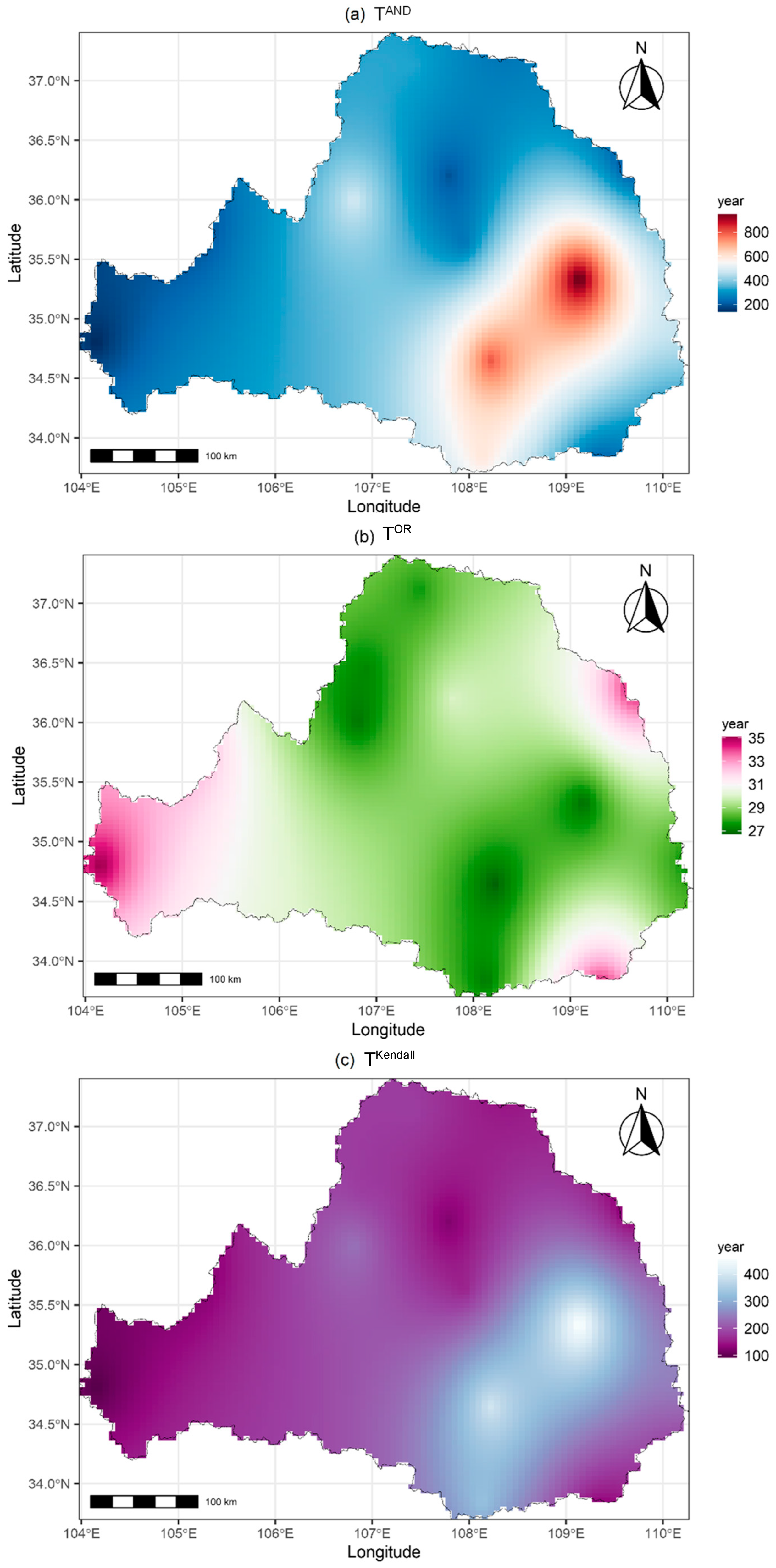
Figure 5 displays the spatial variations in the joint return periods in AND, OR, and Kendall for the SPI and SPEI with a 50-year RP in the Wei River basin, which are also interpolated with the Kriging method. Due to the distinct dependence patterns between the SPI and SPEI across the basin, the joint return periods in AND, OR, and Kendall exhibit different spatial variation features. As observed in Figure 5, the western and central-northern regions are more prone to experiencing simultaneous severe droughts characterized by both the SPI and SPEI with the T^AND return periods less than 400 years. In contrast, the central-southeastern part has relatively fewer chances of experiencing simultaneous SPI- and SPEI-based droughts with the T^AND return period potentially exceeding 800 years. The spatial variations in TOR present a different feature compared to T^AND. It indicates that the western, northeastern, and southeastern regions are less likely to encounter a 50-year drought represented solely by either the SPI or SPEI, while the central-southeastern and northwestern regions are more likely to experience a 50-year SPI or SPEI drought. Regarding T^Kendall, as shown in Figure 5c, its spatial variations are similar to those of T^AND but with relatively shorter return periods. This suggests that the basin may experience compound drought events with shorter recurrence intervals, highlighting the possibility of concurrent extreme drought occurrences based on the interdependence between the SPI and SPEI.

These spatial variation features of the joint return periods emphasize the complex and region-specific nature of drought risks in the Wei River basin. Understanding these variations is crucial for developing targeted drought management strategies and implementing adaptive measures in different regions to enhance the basin’s resilience to drought events. Policymakers and water resource managers can utilize this information to prioritize drought mitigation efforts and allocate resources effectively, considering both individual and joint drought occurrences in the region.

5. Conclusions

In this study, we conducted a comprehensive multivariate drought risk analysis in the Wei River basin using copula methods, specifically comparing the performances of parametric and nonparametric copulas. Our findings shed light on the interdependence between the standardized precipitation index (SPI) and the standardized precipitation evapotranspiration index (SPEI) and their implications for drought risk assessment in the region.

Through the selection of appropriate copula functions and marginal distributions, we quantified the joint probabilistic characteristics of the SPI and SPEI, enabling us to identify the most suitable copula models for each station. Our results demonstrated that the generalized extreme value (GEV) distribution was predominantly identified as the most appropriate marginal model for both the SPI and SPEI. The Gaussian copula emerged as the primary selection among the parametric copula models, while the nonparametric copulas only showed better performance at one out of eighteen meteorological stations in capturing the interdependence between the variables.

The joint return periods, including T^OR, T^AND, and Kendall’s return period (T^Kendall), provided valuable insights into the co-occurrence of extreme drought events. We observed varying spatial patterns in the basin with certain regions more prone to experiencing concurrent drought conditions characterized by both the SPI and SPEI. Our spatial analysis also revealed that the SPEI exhibited more severity in drought characterization than the SPI, highlighting the significance of considering both precipitation and temperature factors in drought assessments. The disparities in the spatial features of the SPI and SPEI underscore the need for a comprehensive approach that incorporates multiple meteorological variables to enhance drought risk analysis accuracy. Overall, our study contributes to a better understanding of the drought patterns and their joint risks in the Wei River basin. The copula-based approach demonstrated its effectiveness in quantifying the interdependence between the SPI and SPEI, providing valuable information for water resource management and drought resilience planning in the region. The insights gained from this research can serve as a basis for informed decision-making and the development of targeted drought mitigation and adaptation strategies. Policymakers and water resource managers can utilize this knowledge to implement region-specific measures and policies to combat the increasing drought risks in the basin effectively.

In conclusion, our study showcases the value of copula methods, including both parametric and nonparametric copulas, in multivariate drought risk analysis and emphasizes the importance of considering joint drought occurrences to enhance drought preparedness and water management strategies in the Wei River basin. Moreover, parametric copulas would be sufficient to analyze multivariate drought risks in the Wei River basin for most cases. Additionally, the comparison of parametric and nonparametric copulas for quantifying the interdependence between the 3-month SPI and SPEI is presented in Table S3. The results also demonstrated the applicability of the parametric copulas on investigating long-term multivariate drought risks. As climate change continues to influence hydrological patterns, non-stationarity may exist in both the SPI and SPEI series. Consequently, more studies are required to explore whether parametric copulas would still have better performances than nonparametric models under nonstationary conditions.

References

1. Wilhite, D.A. (Ed.) Drought as a natural hazard: Concepts and definitions. In Drought: A Global Assessment; Routledge: London, UK, 2000; Chapter 1; Volume I, pp. 3–18. [Google Scholar]
2. Mishra, A.K.; Singh, V.P. A review of drought concepts. J. Hydrol. 2010, 391, 202–216. [Google Scholar]
3. McKee, T.B.; Doesken, N.J.; Kleist, J. The relationship of drought frequency and duration to time scales. In Proceedings of the 8th Conference on Applied Climatology, Anaheim, CA, USA, 17–22 January 1993. [Google Scholar]
4. Vicente-Serrano, S.M.; Beguería, S.; López-Moreno, J.I. A multiscalar drought index sensitive to global warming: The standardized precipitation evapotranspiration index. J. Clim. 2010, 23, 1696–1718. [Google Scholar] [CrossRef]
5. Beguería, S.; Vicente-Serrano, S.M.; Reig, F.; Latorre, B. Standardized precipitation evapotranspiration index (SPEI) revisited: Parameter fitting, evapotranspiration models, tools, datasets and drought monitoring. Int. J. Climatol. 2014, 34, 3001–3023. [Google Scholar] [CrossRef]
6. Li, X.; Sha, J.; Wang, Z.L. Comparison of drought indices in the analysis of spatial and temporal changes of climatic drought events in a basin. Environ. Sci. Pollut. Res. 2019, 26, 10695–10707. [Google Scholar] [CrossRef] [PubMed]
7. Chong, K.L.; Huang, Y.F.; Koo, C.H.; Ahmed, A.N.; El-Shafie, A. Spatiotemporal variability analysis of standardized precipitation indexed droughts using wavelet transform. J. Hydrol. 2022, 605, 127299. [Google Scholar] [CrossRef]
8. Huang, Y.F.; Ahmed, A.N.; Ng, J.L.; Tan, K.W.; Kumar, P.; El-Shafie, A. Rainfall Variability Index (RVI) analysis of dry spells in Malaysia. Nat. Hazards 2022, 112, 1423–1475. [Google Scholar] [CrossRef]
9. Yong, S.L.S.; Ng, J.L.; Huang, Y.F.; Ang, C.K.; Mirzaei, M.; Ahmed, A.N. Local and global sensitivity analysis and its contributing factors in reference crop evapotranspiration. Water Supply 2023, 23, 1672–1683. [Google Scholar] [CrossRef]
10. Hao, Z.; AghaKouchak, A. Multivariate standardized drought index: A parametric multi-index model. Adv. Water Resour. 2013, 57, 12–18. [Google Scholar] [CrossRef]
11. Kao, S.C.; Govindaraju, R.S. A copula-based joint deficit index for droughts. J. Hydrol. 2010, 380, 121–134. [Google Scholar] [CrossRef]
12. Serinaldi, F.; Kilsby, C.G. Stationarity is undead: Uncertainty dominates the distribution of extremes. Adv. Water Resour. 2015, 77, 17–36. [Google Scholar]
13. Wang, F.; Wang, Z.; Yang, H.; Di, D.; Zhao, Y.; Liang, Q. A new copula-based standardized precipitation evapotranspiration streamflow index for drought monitoring. J. Hydrol. 2020, 585, 124793. [Google Scholar] [CrossRef]
14. De Michele, C.; Salvadori, G.; Vezzoli, R.; Pecora, S. Multivariate assessment of droughts: Frequency analysis and dynamic return period. Water Resour. Res. 2013, 49, 6985–6994. [Google Scholar] [CrossRef]
15. Xiao, M.; Yu, Z.; Zhu, Y. Copula-based frequency analysis of drought with identified characteristics in space and time: A case study in Huai River basin, China. Theor. Appl. Climatol. 2019, 137, 2865–2875. [Google Scholar] [CrossRef]
16. Huang, K.; Fan, Y.R. Parameter Uncertainty and Sensitivity Evaluation of Copula-Based Multivariate Hydroclimatic Risk Assessment. J. Environ. Inform. 2021, 38, 131–144. [Google Scholar] [CrossRef]
17. Fan, Y.R.; Yu, L.; Shi, X.; Duan, Q.Y. Tracing uncertainty contributors in the multi-hazard risk analysis for compound extremes. Earth’s Future 2021, 9, e2021EF002280. [Google Scholar] [CrossRef]
18. Zhou, X.; Huang, G.; Wang, X.; Fan, Y.; Cheng, G. A coupled dynamical-copula downscaling approach for temperature projections over the Canadian Prairies. Clim. Dyn. 2018, 51, 2413–2431. [Google Scholar] [CrossRef]
19. Salvadori, G.; De Michele, C. On the Use of Copulas in Hydrology: Theory and Practice. J. Hydrol. Eng. 2007, 12, 369–380. [Google Scholar] [CrossRef]
20. Song, S.; Singh, V.P. Meta-elliptical copulas for drought frequency analysis of periodic hydrologic data. Stoch. Environ. Res. Risk Assess. 2010, 24, 425–444. [Google Scholar] [CrossRef]
21. Kolev, N.; dos Anjos, U.; de M. Mendes, B.V. Copulas: A Review and Recent Developments. Stoch. Models 2006, 22, 617–660. [Google Scholar] [CrossRef]
22. Latif, S.; Simonovic, S.P. Nonparametric Approach to Copula Estimation in Compounding the Joint Impact of Storm Surge and Rainfall Events in Coastal Flood Analysis. Water Resour. Manag. 2022, 36, 5599–5632. [Google Scholar] [CrossRef]
23. Latif, S.; Simonovic, S.P. Trivariate Joint Distribution Modelling of Compound Events Using the Nonparametric D-Vine Copula Developed Based on a Bernstein and Beta Kernel Copula Density Framework. Hydrology 2022, 9, 221. [Google Scholar] [CrossRef]
24. Zhang, L.; Singh, V.P. Copulas and Their Applications in Water Resources Engineering; Cambridge University Press: New York, NY, USA, 2019. [Google Scholar]
25. Fan, Y.R.; Huang, W.W.; Li, Y.P.; Huang, G.H.; Huang, K. A coupled ensemble filtering and probabilistic collocation approach for uncertainty quantification of hydrological models. J. Hydrol. 2015, 530, 255–272. [Google Scholar] [CrossRef]
26. Fan, Y.R. Bivariate hydrologic risk analysis for the Xiangxi River in Three Gorges Reservoir Area, China. Environ. Syst. Res. 2022, 11, 18. [Google Scholar] [CrossRef]
27. Nagler, T. kdecopula: An R Package for the Kernel Estimation of Bivariate Copula Densities. J. Stat. Softw. 2018, 84, 1–22. [Google Scholar] [CrossRef]
28. Aitken, C.G.G.; Lucy, D. Evaluation of Trace Evidence in the Form of Multivariate Data. J. R. Stat. Soc. C 2004, 53, 109–122. [Google Scholar] [CrossRef]
29. Gijbels, I.; Mielniczuk, J. Estimating the Density of a Copula Function. Commun. Stat.-Theory Methods 1990, 19, 445–464. [Google Scholar] [CrossRef]
30. Charpentier, A.; Fermanian, J.D.; Scaillet, O. The Estimation of Copulas: Theory and Practice. In Copulas: From Theory to Application in Finance; Rank, J., Ed.; Risk Books: London, UK, 2007. [Google Scholar]
31. Graler, B.; van den Berg, M.J.; Vandenberghe, S.; Petroselli, A.; Grimaldi, S.; De Baets, B.; Verhoest, N.E.C. Multivariate return periods in hydrology: A critical and practical review focusing on synthetic design hydrograph estimation. Hydrol. Earth Syst. Sci. 2013, 17, 1281–1296. [Google Scholar] [CrossRef]
32. Salvadori, G.; De Michele, C.; Kottegoda, N.T.; Rosso, R. Extremes in Nature: An Approach Using Copula; Springer: Dordrencht, The Netherlands, 2007; p. 292. [Google Scholar]
33. Sraj, M.; Bezak, N.; Brilly, M. Bivariate flood frequency analysis using the copula function: A case study of the Litija station on the Sava River. Hydrol. Process. 2015, 29, 225–238. [Google Scholar] [CrossRef]
34. Zou, L.; Xia, J.; She, D. Analysis of Impacts of Climate Change and Human Activities on Hydrological Drought: A Case Study in the Wei River Basin, China. Water Resour. Manag. 2018, 32, 1421–1438. [Google Scholar] [CrossRef]
35. Chang, J.; Li, Y.; Wang, Y.; Yuan, M. Copula-based drought risk assessment combined with an integrated index in the Wei River Basin, China. J. Hydrol. 2016, 540, 824–834. [Google Scholar] [CrossRef]
36. Wen, Y.; Yang, A.; Fan, Y.; Wang, B.; Scott, D. Stepwise cluster ensemble downscaling for drought projection under climate change. Int. J. Climatol. 2023, 43, 2318–2338. [Google Scholar] [CrossRef]
37. Wang, Q.; Zhang, R.; Qi, J.; Zeng, J.; Wu, J.; Shui, W.; Wu, X.; Li, J. An improved daily standardized precipitation index dataset for mainland China from 1961 to 2018. Sci. Data 2022, 9, 124. [Google Scholar] [CrossRef] [PubMed]
38. Wang, Q.; Zeng, J.; Qi, J.; Zhang, X.; Zeng, Y.; Shui, W.; Xu, Z.; Zhang, R.; Wu, X.; Cong, J. A multi-scale daily SPEI dataset for drought characterization at observation stations over mainland China from 1961 to 2018. Earth Syst. Sci. Data 2021, 13, 331–341. [Google Scholar] [CrossRef]
39. Droogers, P.; Allen, R.G. Estimating Reference Evapotranspiration Under Inaccurate Data Conditions. Irrig. Drain. Syst. 2002, 16, 33–45. [Google Scholar] [CrossRef]
40. Şen, Z.; Almazroui, M. Actual Precipitation Index (API) for Drought classification. Earth Syst. Environ. 2021, 5, 59–70. [Google Scholar] [CrossRef]
Figure 1. The location of the Wei River basin.
Water 15 03283 g001
Figure 2. The procedures for multivariate drought risk analysis.
Water 15 03283 g002
Figure 3. Temporal variations in the SPI and SPEI at stations 52986 and 52996.
Water 15 03283 g003
Figure 4. Spatial variation in the SPI and SPEI with a return period of 50 years.
Water 15 03283 g004
Figure 5. Spatial variation in joint return periods for the SPI and SPEI with a 50-year RP.
Water 15 03283 g005