Article

Significant Increases in Water Vapor Pressure Correspond with Climate Warming Globally

1
Center for Agricultural Water Research in China, College of Water Resources and Civil Engineering, China Agricultural University, Beijing 100083, China
2
College of Water Sciences, Beijing Normal University, Beijing 100875, China
*
Author to whom correspondence should be addressed.
Water 2023, 15(18), 3219; https://doi.org/10.3390/w15183219
Submission received: 2 August 2023 / Revised: 4 September 2023 / Accepted: 7 September 2023 / Published: 10 September 2023
(This article belongs to the Section Hydrology)

Abstract

:
Global warming has become indisputable in recent years; however, the mechanisms by which water vapor, radiation, and greenhouse gases such as carbon dioxide contribute to driving global warming remain unclear, and it is becoming increasingly important to clarify their respective effects on temperature warming. In this study, we used the Global Land Data Assimilation System (GLDAS) datasets and National Oceanic and the Atmospheric Administration (NOAA) Global Monitoring Laboratory (GML) data to investigate the spatiotemporal variation characteristics of global warming and its driving mechanisms. The effects of water vapor, radiation (net longwave radiation), and CO2 on temperature rise are quantified from the perspective of the coupled land–atmosphere system, and water vapor is characterized in terms of the vapor pressure deficit (difference between saturated and actual water vapor pressures) to explicitly characterize its impact on the global water–heat cycle. The results show the following: (1) Under significant global warming, the vapor pressure deficit (VPD) exhibits an increasing trend, which is attributed to the rate of increase in actual water vapor being relatively slower than saturated water vapor. (2) Compared with the significant positive contribution of water vapor to global warming, CO2 is not, as generally expected, the most critical greenhouse gas causing global warming. (3) Water vapor and net longwave radiation (NLR) have significant mutual feedbacks on global warming. (4) A remarkable complementary mechanism of global warming that involves water vapor and NLR was identified, whereby the increased saturated water vapor induced by the rising temperature dominates the decrease in NLR. The results from this study have important theoretical value by enabling a more complete understanding of the contribution of VPD to global climate change and shedding light on the large-scale water vapor–climate change mutual feedback mechanism through research.

1. Introduction

Global warming has become an indisputable fact and one of the biggest challenges facing human development since the new millennium [1,2]. It results in negative effects on both humans and nature, such as economic downturn [3,4], increased marine mammal vulnerability [5], increased ENSO (El Niño-Southern Oscillation) variability [6], and decreased crop yields [7], among numerous others. When it comes to global warming, increased carbon dioxide, ozone, and methane usually attract great attention. In contrast, water vapor emissions from human sources are insignificant compared to those from natural sources. However, this does not mean that water vapor overall has little effect on the environment and climate. As the most active factor in the global water cycle [8], water vapor is responsible for two-thirds of global warming [9] and it absorbs the most significant longwave radiation from the ground [10], which is closely related to the earth surface energy budget and plays an important role in global climate change, especially in arctic areas [11,12,13]. With the continuous intensification of global warming, the atmospheric water vapor content increases and further leads to a stronger greenhouse effect and enhancement of downward longwave radiation (DLR), which constitutes the positive feedback of the water–heat cycle. This feedback can also be amplified by other greenhouse gases; for example, increased carbon dioxide will cause more water vapor to enter the atmosphere [14,15]. Therefore, an in-depth understanding of the feedback effect of water vapor and DLR on global warming not only contributes to the study of climate change, but also provides a theoretical basis for the effective use of water resources.
Recently, many studies on water vapor and DLR have mainly focused on describing the phenomenon and providing basic facts, leaving a research gap in terms of the function of the two variables in global warming. Wang et al. [16] analyzed the characteristics of the summer water vapor content in northwest China and concluded that atmospheric water vapor has a significant and regional positive feedback effect on the surface air temperature. Liu et al. studied the dependence of temperature warming and altitude on the Qinghai–Tibet Plateau and other parts of China and found that climate warming has a good correlation with the variability in water vapor at different altitudes [17,18]. In other parts of the world, such as the Arctic, the temperature has warmed more than twice as much as the global average, which is also linked to increased water vapor in the atmosphere [19]. The above research has been on a regional rather than global scale and, therefore, systematic and comprehensive results are lacking.
In addition, the mechanisms of water vapor, CO2, and radiation on global warming are still unclear. The study of Gao et al. concluded that global warming is mainly caused by the absorption of longwave radiation from abundant water vapor at levels above 3 km from the ground [18,20]. However, since the abundance of water vapor in the stratosphere decreased after 2000 [21,22], whether there still exists a feedback effect between water vapor and the surface temperature is unclear. Some scholars thought that the stratospheric water vapor (SWV) feedback was significant since the temperature kept increasing [23], while some argued that the feedback effect of SWV was not as significant as previously considered [24,25]. Thus, the mutual mechanism due to the combination of water vapor and DLR as a function of global warming must be explored, which is crucial for our understanding of the contribution of CO2 and other traditional greenhouse gases to climate change and can also provide technical support for research on the atmospheric water vapor–climate change mutual feedback mechanism at different spatiotemporal scales.
The vapor pressure deficit (VPD), calculated as the difference between saturated and actual water vapor pressure, was used as an important indicator of atmospheric drought. We use the VPD to accurately describe atmospheric water vapor variations. The negative effect of an increased VPD on vegetation is confirmed at global as well as regional scales, and to some extent offsets the increase in carbon uptake caused by the effect of CO2 fertilization [26,27]. However, many existing findings only separately consider the effects of either the VPD, CO2, or DLR on the climate system and hydrosphere cycle, since both have an impact on plant growth, crop yield, etc. [28,29,30,31]. Thus, explicitly characterizing the impacts of VPD and DLR on the global water–heat cycle is an important contribution to addressing the impacts of global climate change.
In summary, as the most active factor in the climate system and hydrosphere cycle and the most critical factor affecting extreme weather events such as drought and flood, atmospheric water vapor plays a vital role in the global energy and water cycle. The objectives of this study are: (1) to investigate the spatiotemporal variation characteristics of global warming and associated water–heat elements, (2) to comparatively quantify the influence of VPD and CO2 on the greenhouse effect, represented by the rising air temperature from the perspective of the land–atmosphere coupling system, and (3) to explore the mutual feedback mechanism between water vapor, longwave radiation, and global warming. The results of this study will advance our understanding of global warming and contribute to the sustainable development of water resources.

2. Materials and Methods

2.1. Data

2.1.1. GLDAS NOAH Data

The Global Land Data Assimilation System (GLDAS, see Abbreviations) is a joint development of NASA’s Goddard Space Flight Center (GSFC) and the National Oceanic and Atmospheric Administration’s (NOAA) National Center for Environmental Prediction (NCEP). Compared with other remote sensing data, GLDAS data have higher spatial and temporal resolution and good applicability in evaluating global and regional changes in environmental factors, such as land water storage, soil water content, and regional droughts [32]. This study used GLDAS-2.0 data (https://disc.gsfc.nasa.gov/datasets/GLDAS_NOAH025_M_2.0/summary?keywords=GLDAS (accessed on 17 June 2023)), which have good time continuity, high reliability, and good applicability for meteorological and hydrological research at a global scale [33]. The monthly data of NOAH LSM selected in this study have a spatial resolution of 0.25° and contain 36 variables. The time range is from January 1970 to December 2010.

2.1.2. NOAA GML Data

The NOAA Global Monitoring Laboratory (GML) mainly focuses on greenhouse gas and carbon cycle feedback, changes in cloud, aerosol, and surface radiation, and the restoration of stratospheric ozone. GML’s annual and monthly data of global average CO2, measured at four observatories in Barrow, Alaska; American Samoa; Mauna Loa, Hawaii; and Antarctica, in addition to similar data measured at sites in other regions around the world (https://www.esrl.noaa.gov/gmd/ccgg/trends/gl_data.html (accessed on 17 June 2023)), were used in this study. The air samples were collected into glass flasks, and the CO2 content in the air was measured using a semi-automatic, nondispersive infrared flask analyzer to analyze the carbon dioxide concentration of the samples [34].

2.1.3. AVHRR NDVI Data

NDVI3g is the normalized difference vegetation index (NDVI) dataset from advanced very-high-resolution radiometer (AVHRR) instruments, made available by NASA’s Global Inventory Modeling and Monitoring Study third-generation dataset (GIMMS3g) group (https://iridl.ldeo.columbia.edu/SOURCES/.NASA/.ARC/.ECOCAST/.GIMMS/.NDVI3g/.v1p0/datasetdatafiles.html (accessed on 17 June 2023)). It extends from 1981 to 2015, with spatial resolution of 1/12 degree. Each dataset contains 15 days of average NDVI [35].

2.2. Methods

2.2.1. Linear Regression Model

As a statistical analysis method for modeling the relationship between two or more variables in mathematical statistics, the linear regression model has been widely used for trend analysis of hydrometeorological elements [36,37]. The formula is as follows:
y = b   ·   x + a
where y is the annual average air temperature in this study, x represents the year, b is the regression coefficient showing the direction and magnitude of the time change, and a is the regression constant. A positive slope ( b   > 0) indicates that the global air temperature is rising, while a negative slope ( b   < 0) indicates that the global air temperature is declining.

2.2.2. Pearson Correlation Analysis

In this study, Pearson correlation analysis was used to explore the influence of climatic factors such as the vapor pressure deficit, longwave radiation, and surface pressure on air temperature. The formula for calculating the Pearson correlation coefficient is as follows:
  r x y = i = 1 n ( x i x ¯ ) ( y i y ¯ ) i = 1 n ( x i x ¯ ) 2 i = 1 n ( y i y ¯ ) 2
where n is the number of data pairs, x i and y i are two pairs of data, x ¯ and y ¯ are the average values corresponding to each set of data, and r x y reflects the correlation between two variables and ranges between −1 and 1. An absolute value close to 1 indicates a higher correlation.

2.2.3. Partial Correlation Analysis

Partial correlation analysis can be used for regression modeling under the condition that the independent variables are significantly correlated, and it has a wide range of applications in hydrological correlation analysis [38,39,40]. Partial correlation analysis can eliminate the quantitative contribution to the temperature impact resulting from a strong correlation between climate variables. The formula for calculating the partial correlation coefficient is as follows:
r x y , z = r x y r x z r y z ( 1 r x z 2 ) ( 1 r y z 2 )
where r x y , z is the partial correlation coefficients of variables x and y , which eliminate the influence of variable z , and r x y , r x z , and r y z are the Pearson correlation coefficients between variables x and y , x and z , y and z .

2.2.4. Mann–Kendall Nonparametric Test

The purpose of the Mann–Kendall (M–K) test is to statistically evaluate whether the hydrological and climate variables have a monotonic upward or downward trend over time. A monotonic increase (decrease) trend means that the variable increases (decreases) over time. Sen’s slope combined with the Mann–Kendall test is an effective trend analysis method [41,42].
For a set of data series with time x i = ( x 1 , x 2 , , x n ) , β represents Sen’s slope, and the formula is as follows:
β = M e d i a n ( x j x i j i )
where 1 < j < i < n, and a positive β indicates an upward trend while a negative β indicates a downward trend.
To calculate variable S , the formula is as follows:
S = j 1 n 1 i j + 1 n s g n ( x i x j )
where:
s g n x i x j = 1 ,   x i x j > 0 0 ,   x i x j = 0 1 ,     x i x j < 0
If S > 0, then the observation value of the latter part will tend to be larger than the previous observation value; if S   < 0, the observation value of the latter part will tend to be smaller than the previous observation value. If the sample size n   > 10, then the variance, V A R ( S ) , is calculated with the following formula:
V A R ( S ) = n n 1 2 n + 5 t t ( t 1 ) ( 2 t + 5 ) 18
where   t is the extent of any given tier, V A R ( S ) represents the change of S , and the statistic Z M K is then calculated using the following formula:
Z M K = S 1 V A R S ,   S > 0   0   ,   S = 0 S + 1 V A R ( S ) ,   S < 0
Positive (negative) Z M K indicates that the data tend to increase (decrease) over time. If Z M K Z 1 α 2 , reject the null hypothesis H 0 and accept the alternative hypothesis H a . Here, α is the significance level, which was 0.1 in this study.

2.2.5. Calculation of Vapor Pressure Deficit

The VPD is the difference between the saturated and actual water pressure in the air at a certain temperature and reflects the degree of actual water vapor saturation [43]. The VPD is calculated as follows:
V P D = e S T a e a
where e S ( T a ) is the saturated vapor pressure (kPa) when the air temperature is T a , and e S is the actual water pressure (kPa). There are many calculation formulas for e S , such as the Goff–Gratch equation, the Magnus empirical formula, and its improved form, the Tetens formula, among others. This study adopted the formula that has been widely used to calculate the average saturated water pressure for plant evapotranspiration [44]:
e S T i = 0.6108 exp 17.27 × T i T i + 237.3
where T i is the temperature T a ( ° C ) or the dew point temperature T d e w ( ° C ) . The actual water pressure, e a (kpa), can be derived from the following formula:
q = 622 e a p 0.378 e a
where q is specific humidity (kg/kg) and p is atmospheric pressure (kpa).

3. Results

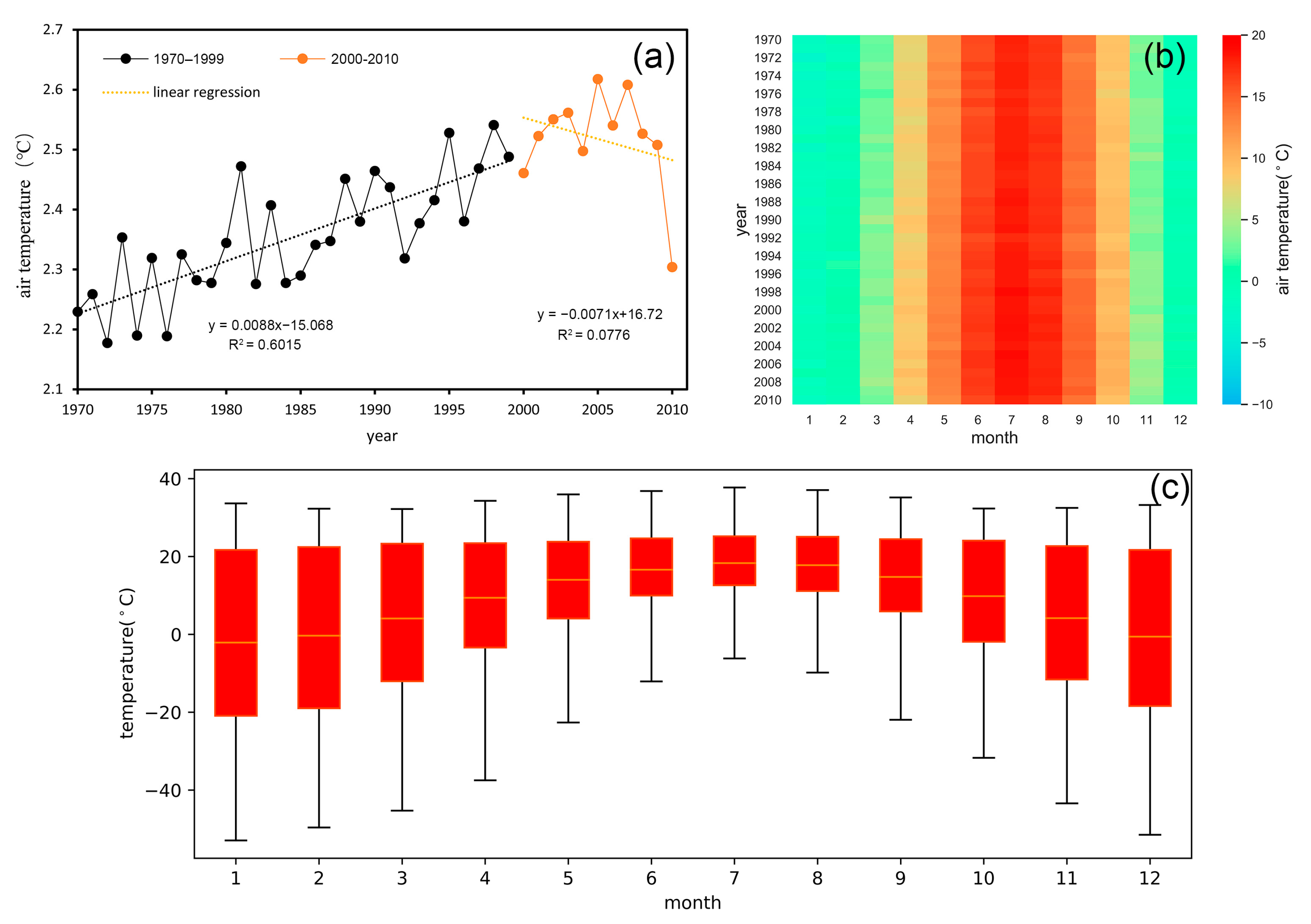
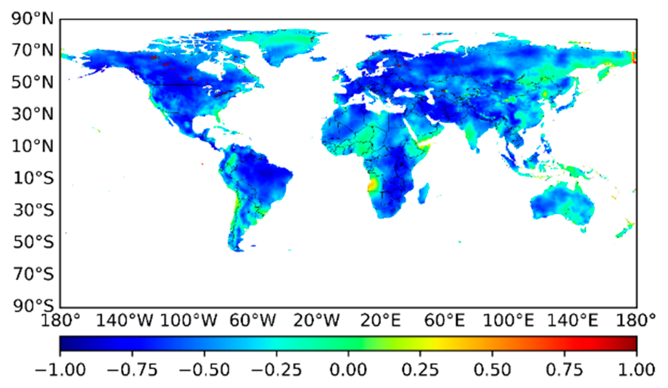
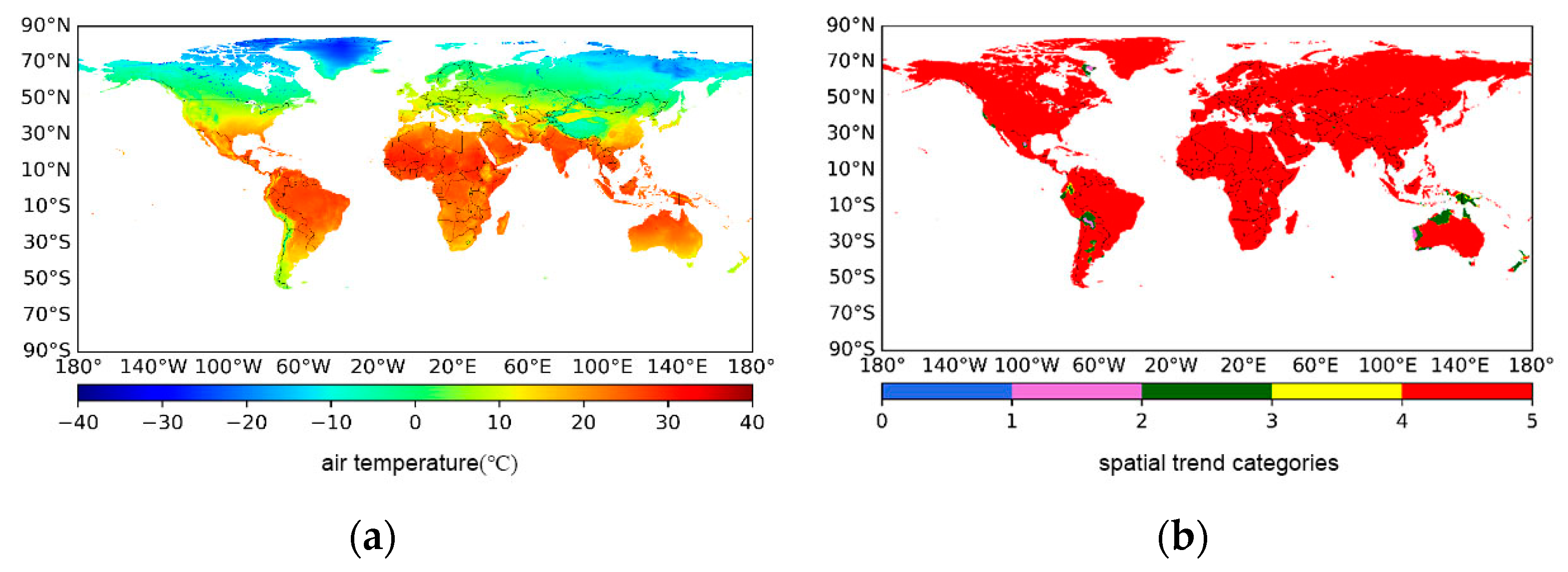
3.1. Spatiotemporal Characteristics of Global Warming

As shown in Figure 1a, the global air temperature showed a significant upward trend from 1970 to 2010 with a rate of 0.009 °C/a, which was consistent with climate warming demonstrated by the Intergovernmental Panel on Climate Change (IPCC) [45]. Moreover, according to Yuan et al. [46,47], the global water use efficiency and the effect of CO2 fertilization tend to be saturated from 2000 onwards, so we used 2000 as the dividing year to discuss the changes in global temperature before and after. It could be seen that the global air temperature has exhibited a downward trend since the new millennium, decreasing at a rate of 0.007 °C/a, which is consistent with the slowdown in global warming since 1999 [48,49,50]. However, such a warming hiatus is only temporary and will not fundamentally change the situation of global warming [51]. The World Meteorological Organization also demonstrated that the global temperatures for each year from 2015 to 2019 were the hottest five years in the entire record, and that global warming is projected to sharply accelerate [52].
As shown in Figure 1b,c, compared with the significant increasing trend of annual mean air temperature, the variation pattern of monthly air temperature at a global scale was relatively stable during the period 1970–2010, which began to consistently increase in February, reached the highest point in July, and began to decline in August. The high-temperature months were concentrated in May to September, while the low-temperature months were concentrated in November to February. In addition, the global air temperature from November to February showed a larger variation range than that from June to August, indicating a more significant response of low temperature to climate warming.
The spatial distribution of the global average multi-year temperature from 1970 to 2010 is illustrated in Figure 2a, which spatially indicated that the average temperature is above 0 °C in most areas. Areas with temperatures greater than 20 °C account for 33.03% of the globe, mainly concentrated within 20° on both sides of the equator. Areas with temperatures below 0 °C account for 32.52% of the globe, mainly concentrated in areas above 50 °C north latitude and on the Tibetan Plateau in China.
The M–K nonparametric test was adopted in this study to analyze the variation trend of the global average air temperature from 1970 to 2010. The results are shown in Figure 2b. The variation trend of the global air temperature was divided into five types, as shown in Table 1. More than 95% of the world’s land surface air temperature showed an upward trend (significant warming and slight warming). This finding is consistent with the conclusion obtained by Ma et al. using the M–K test on data of the US National Climate Data Center [53], and essentially consistent with the general background of global warming analyzed by the linear regression model in Section 3.1. However, there are also spatial differences in global warming. As can be seen from Figure 2b, about 2% of the world’s land surface showed a downward trend (significant cooling and slight cooling), mainly in northwestern Australia and South America, in places such as Bolivia and Argentina, which is consistent with the research results of Ji et al. [54]. They found that certain areas tend to become colder in the context of global warming, such as the Andes in the southern equatorial region.

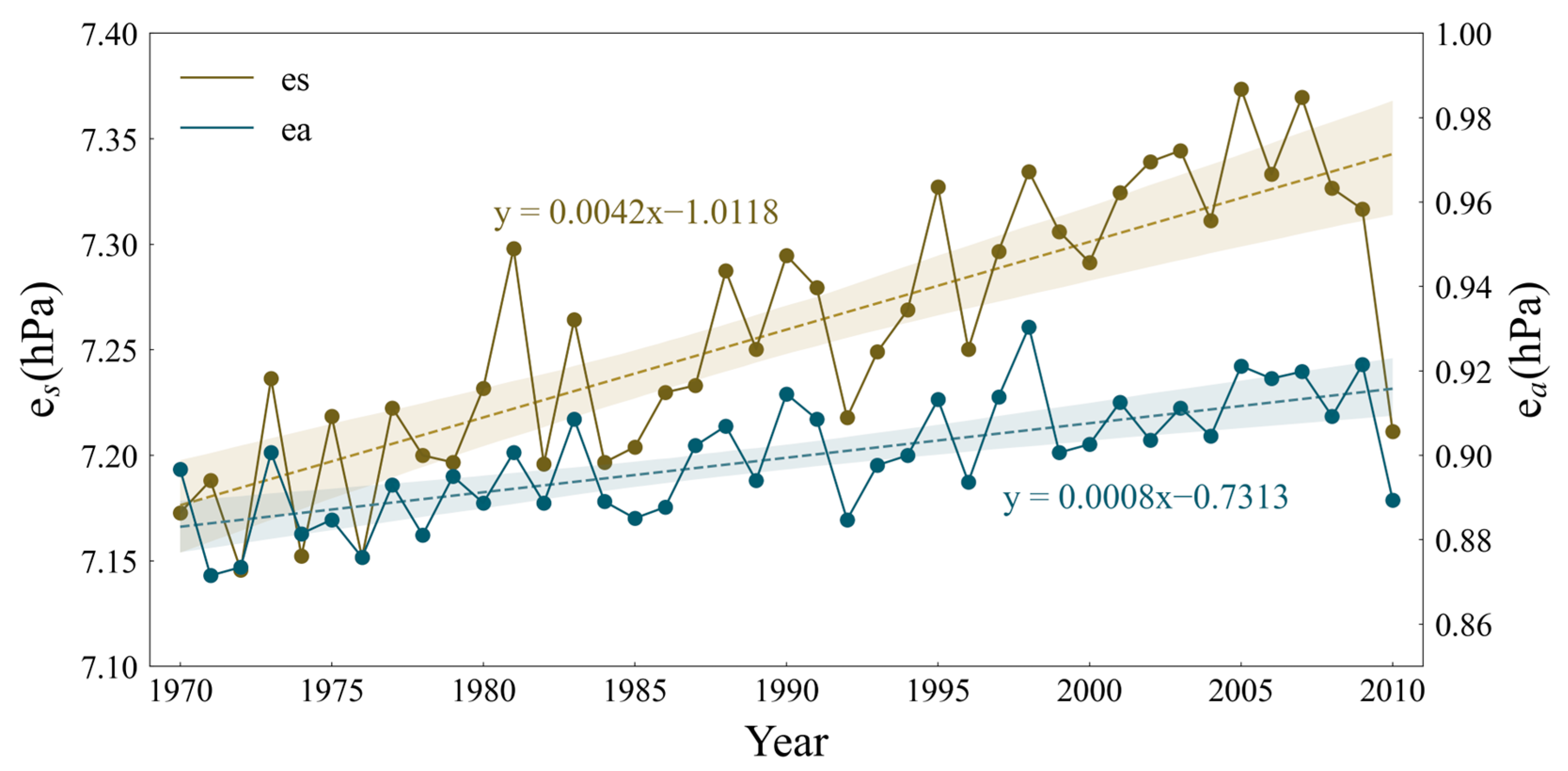
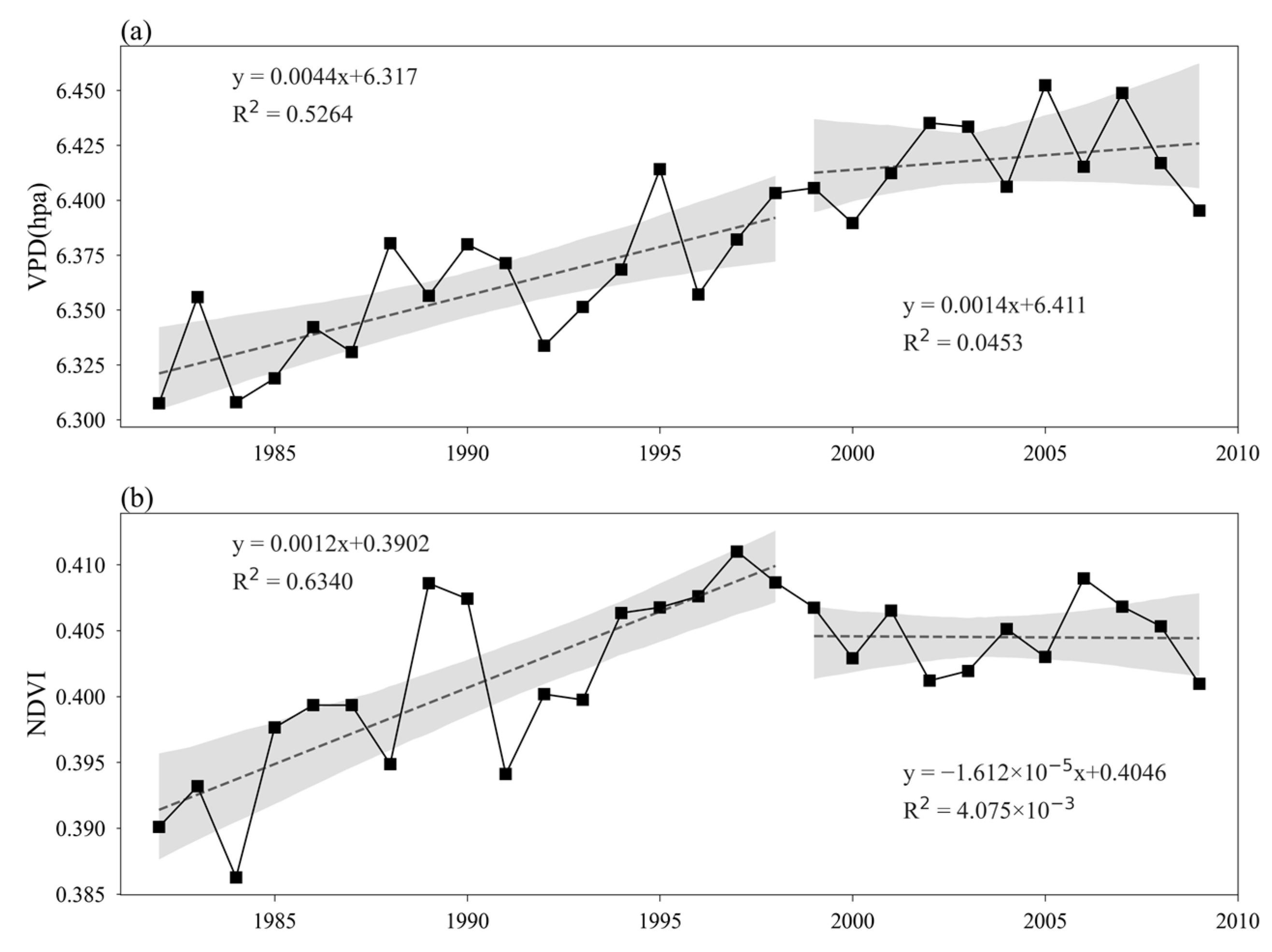
3.2. Variations in Climate Factors Characterizing Water Vapor

According to Formula (9), the determinants of the VPD are saturated vapor pressure, e S , and actual water pressure, e a . We have already described the trends in e S and e a (Figure 3). Both e a and e s show a fluctuating upward trend over time; however, e a grows at a lower rate than e s . In this study, specific humidity, the vapor pressure deficit (VPD), and evapotranspiration (ET) were selected to characterize the temporal and spatial patterns of water vapor. In addition, surface DLR, which is closely associated with water vapor and air temperature, was also selected for exploration.
As shown in Figure 4a, the global average annual specific humidity showed an overall upward trend from 1970 to 2010, increasing at a rate of 0.002/a, which synchronized with the changing pattern of global air temperature, indicating the important role of temperature in changes of specific humidity [47,55].
As shown in Figure 4b, the global annual average VPD exhibited an upward trend from 1970 to 2010, increasing at a rate of 0.003 hpa/a. Similar to specific humidity, changes in VPD showed good synchronization with those of global air temperature. This phenomenon was also noted by Yuan et al. (2019) [47]. However, the global annual average ET increased slightly (Figure 4c), which might be attributed to the trade-off between the increasing ET from 1982 to 1997 and the decreasing ET since 1998 [56]. In addition, an increase in the VPD often means an increase in water vapor lost to the atmosphere through plant transpiration and soil evaporation. From the comparison of global VPD and ET (Figure 4b,c), it was found that the increase in the global average VPD did not lead to significant changes in ET, implying that plants can perceive the drying air and close their stomata to prevent water loss [57]. As shown in Figure 4d, the global annual average DLR from the surface showed an increasing trend from 1970 to 2010, at a rate of 0.0096 W∙m−2/a. It is noteworthy that DLR values showed consistent and positive correlations with the annual average temperature and specific humidity. This is consistent with the conclusions in the research of Christian et al. [58].

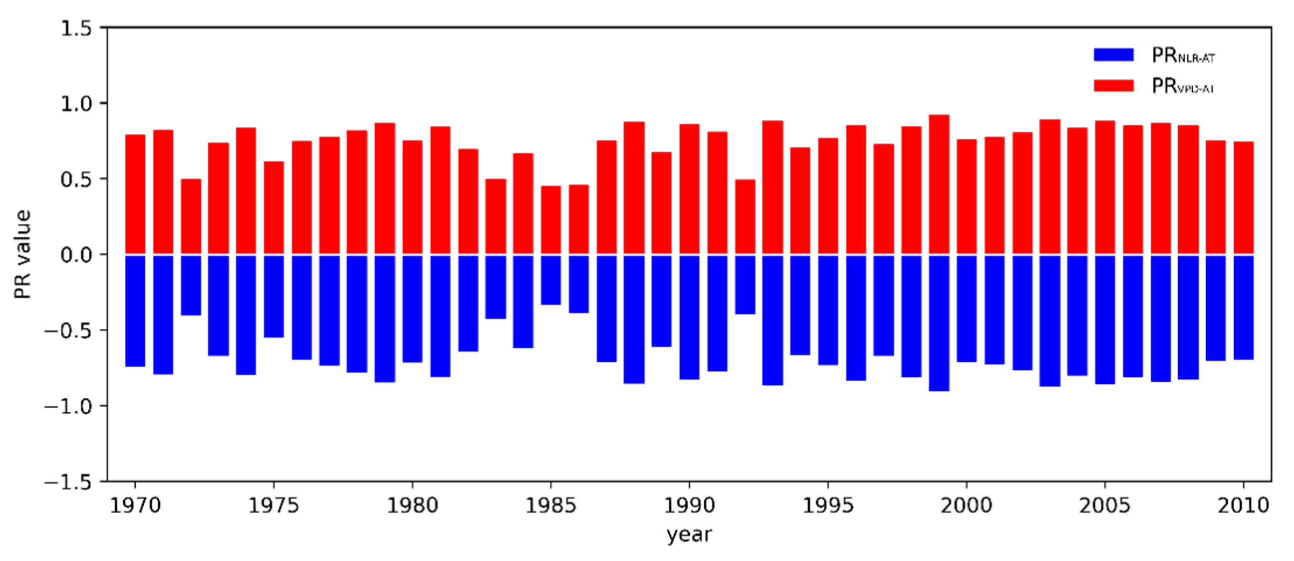
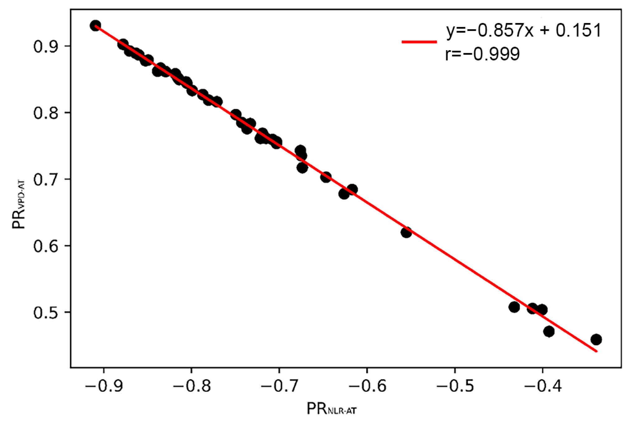
3.3. Increased VPD Determines Global Warming

In addition to specific humidity, ET, VPD, and DLR, the greenhouse gas CO2 was also examined in this study to quantify the relationship between each element and the air temperature for further identification of the key factors contributing to climate warming. In view of the mutual effect mechanism between CO2 and water vapor, and the synchronized variation characteristics of VPD and specific humidity, it is necessary to eliminate the autocorrelation effect of CO2 and water vapor in studying the individual quantitative contribution of these two greenhouse gases to global warming. Partial correlation analysis was adopted in this study to investigate the spatial and temporal relationships between global air temperature, CO2, and VPD, as shown in Figure 5. The partial correlation coefficients of air temperature and VPD from 1970 to 2010 were all greater than 0.9, with an average value of 0.972, while the partial correlation coefficient between temperature and CO2 showed fluctuations from year to year, with an average value of 0.171. This indicates that the contribution of VPD to global warming is significantly greater than that of CO2, confirming that the increased VPD in recent decades has offset the CO2 fertilization effect [26,27]. Similar results were also demonstrated by Hu et al. (2019), who concluded that temperature is more strongly correlated with water vapor than CO2 [40].

3.4. Mutual Effect between Global Warming and Water Vapor

3.4.1. Proposed Framework of Global Warming and Water Vapor Feedback

The response of the air temperature to radiative disturbances due to external factors will result in global warming, while changes in other variables, such as solar radiation and atmospheric composition caused by global warming, will simultaneously cause new radiation disturbances. Such feedback involves various processes, such as water vapor, cloud, ice–albedo, and atmospheric temperature decline feedbacks. Water vapor feedback can significantly affect regional climate sensitivity and amplify the greenhouse effect of other greenhouse gases, and it has the strongest effect on the climate system [59,60]. When the atmospheric water vapor content increases, the DLR released by water vapor will be amplified, increasing the atmospheric temperature, which will cause more water vapor to enter the atmosphere. Exploring the mechanism of the mutual effect between DLR, water vapor, and air temperature is important in understanding and quantifying the contribution of water vapor to global warming.

3.4.2. Quantitative Analysis on Mutual Effect between Global Warming and Water Vapor

Net longwave radiation (NLR) flux is the difference between radiation from the ground and that from the atmosphere (DLR). Increased DLR usually indicates decreased NLR. Due to the mutual mechanism of the combination of longwave radiation as a function of global warming [61,62], an attribution analysis of air temperature rise, as related to NLR, was performed. Figure 6 shows the spatial correlation between NLR and air temperature from 1970 to 2010. There was a significantly negative correlation between NLR and air temperature in most parts of the world. Areas with a correlation coefficient value lower than 0 accounted for 98.11% of the world, and areas with a value lower than −0.5 accounted for 48.30%. Only the Bering Strait region of Russia and the Angola region of Africa showed a significantly positive correlation between NLR and air temperature. Only the eastern part of Russia, the northeastern part of Canada, Indonesia, and the northwestern part of Brazil showed a significantly negative correlation between VPD and air temperature.
To eliminate the mutual influence between VPD and NLR, partial correlation analysis was conducted to identify the independent influence of water vapor and NLR on air temperature. The results are shown in Figure 7 and Figure 8.
As shown in Figure 7, the partial correlation coefficient between air temperature and VPD and NLR from 1970 to 2010 shows maintenance of a good complementary relationship, i.e., the coefficient between VPD and air temperature increased, while the coefficient between NLR and air temperature decreased, and vice versa. Accordingly, Figure 8 shows that PRNLR–AT and PRVPD–AT had a strongly negative correlation (r = −0.999), which further verifies the complementary relationship between NLR and water vapor. This complementary relationship has also been regionally verified.

3.5. Implications from the Response of Vegetation to VPD

As an important driver of the atmospheric water demand for plants, VPD influences terrestrial ecosystem function and photosynthesis, and is also a dominant factor in vegetation productivity [63,64]. Here, we analyzed the relationship between NDVI and VPD. NDVI is based on the spectral characteristics of vegetation, combining satellite visible light and near-infrared bands to form various vegetation indices, reflecting the dynamic changes in vegetation in terms of ecological monitoring and climate change [65]. According to the results obtained by Yuan et al. [47] that emphasized the impact of VPD on vegetation growth, 1999 was used as a turning point to analyze the global relationship between VPD and NDVI.
Figure 9 shows that both VPD and NDVI had an increasing trend before 1999. However, there was a slight increase in VPD from 1999 to 2009, while NDVI showed a downward trend, indicating the inhibition effect of VPD on vegetation. In terms of space, VPD and NDVI were positively correlated in 47.9% of areas before 1999, and negatively correlated in the remaining 52.1%. However, since 1999, the blue areas representing negative correlation, as shown in Figure 10, have increased, with positively correlated areas decreasing to 42.4% of the world and negatively correlated areas thereby increasing to 57.6%, further implying that increased VPD has a certain inhibitory effect on plant growth.

4. Discussion

4.1. Enlightening of VPD and CO2 Effect on Global Warming

Recent studies have shown that the global water use efficiency continued to increase from 1982 to 2000 but has since saturated. This is likely because in most parts of the globe when VPD is too high, plant stomata tend to close in order to reduce water loss, which makes plant photosynthesis weaker and thus leads to partially offsetting the increase in carbon uptake caused by the effect of CO2 fertilization [28,63,66].
VPD is also strongly correlated with climatic variables such as temperature, evapotranspiration, and soil moisture [67,68]. A high VPD tends to be accompanied by a low SM, and the frequency and intensity of composite extreme events of atmospheric drought and soil drought will further increase in the future and have much higher impacts on ecosystem productivity than single extreme events [67].
In addition, VPD can also indirectly drive the atmospheric CO2 growth rate [68,69]. The persistent anomalous changes in VPD have impacts on the climate and ecosystems and pose a challenge for global greening to mitigate the surface temperature rise; thus, it is necessary to conduct in-depth studies to characterize the long-term changes in VPD.

4.2. Uncertainty and Expectations for Future Studies

This paper was based on data from GLDAS NOAH, NOAA GML, and AVHRR NDVI, analyzed using a linear correlation model, Pearson correlation analysis, partial correlation analysis, and the M–K test to identify the main causes of global warming greenhouse gases, study the changes of global temperature and climate elements at the temporal and spatial scale, and quantify the influence of water vapor on the greenhouse effect in the land–atmosphere coupling system, allowing for an overall analysis of the mutual feedback mechanism of water vapor and longwave radiation.
In view of the shortcomings and problems in this study, some clear recommendations emerged, as follows: (1) Collecting multi-source data with higher precision and longer time series is of great significance for future research. (2) This paper studied the mutual feed relationship between water vapor and temperature on a global scale, but the physical mechanism is more complicated in reality; hence, heat flux and other factors need to be considered in additional systematic and rigorous studies. (3) The feedback mechanism between water vapor and global warming was investigated in this study, and the effect of this feedback mechanism on the greenhouse effect of other greenhouse gases should be further explored.

5. Conclusions

Water vapor is an indispensable component of the atmosphere and an essential contributor to global warming. It can significantly affect atmospheric radiative transfer, atmospheric circulation, weather conditions, etc. It can also amplify the greenhouse effect of other greenhouse gases, leading to extreme events such as glacier melting, floods, and droughts. Based on the GLDAS dataset and NOAA GML data, we used linear correlation modeling, partial correlation analysis, and the M–K test to identify the main causes of global warming and their driving mechanisms. The temporal and spatial variations of global temperature and related climate elements were investigated, the impact of water vapor on the greenhouse effect in the coupled land–atmosphere system was quantified, and the mutual feedback mechanism between water vapor and longwave radiation was analyzed. The main conclusions can be summarized as follows:
(1)
From 1970 to 2010, global air temperature, VPD, and specific humidity showed an increasing trend, with a significantly positive correlation. When both the actual water vapor content and the saturated water vapor increased, the rise in the actual water vapor was lower than that of the saturated water vapor pressure.
(2)
Compared with the increasing concentration of CO2, the increased VPD plays a more important role in global warming.
(3)
There was a strong complementary relationship between the contribution of net longwave radiation and water vapor to global warming, and the increase in saturated water vapor dominated the decrease in net longwave radiation.

Author Contributions

Conceptualization, L.L.; methodology, L.L., X.Z. and Y.H.; data curation, Y.H.; validation, X.Z. and L.L.; formal analysis, X.Z. and Y.H.; investigation, Y.H.; resources, L.L.; writing—original draft preparation, Y.H.; writing—review and editing, L.L., X.Z. and H.S.; visualization, Y.C. and X.Z.; supervision, L.L.; funding acquisition, L.L. All authors have read and agreed to the published version of the manuscript.

Funding

This research was jointly funded by the National Natural Science Foundation of China (Nos. 52079138 and 51961145104) and the National Training Program of Innovation and Entrepreneurship for Undergraduates (No. 201910019390).

Data Availability Statement

All data generated or analyzed are included in this published article.

Acknowledgments

The authors are grateful to the Global Land Data Assimilation System team, NASA’s Global Inventory Modeling and Monitoring Study third-generation dataset (GIMMS3g) group, and the NOAA Global Monitoring Laboratory, for making the data freely available.

Conflicts of Interest

The authors declare no conflict of interest.

Abbreviations

AbbreviationFull Name
VPDVapor pressure deficit
GLDASGlobal Land Data Assimilation System
NOAANational Oceanic and Atmospheric Administration
GMLGlobal Monitoring Laboratory
NLRNet longwave radiation
ENSOEl Niño-Southern Oscillation
DLRDownward longwave radiation
RATPAC-ARadiosonde Atmospheric Temperature Products for Assessing Climate dataset A
SWVStratospheric water vapor
GSFCGoddard Space Flight Center
NCEPNational Center for Environmental Prediction
LSMLand surface model
NDVINormalized difference vegetation index
ETEvapotranspiration
ATAir temperature
SHSpecific humidity
PRCO2–ATPartial correlation coefficient between CO2 and air temperature
PRVPD–ATPartial correlation coefficient between VPD and air temperature
PRNLR–ATPartial correlation coefficient between NLR and air temperature

References

  1. Hu, A.G. Global Climate Change and China’s Green Development. Chin. J. Popul. Resour. Environ. 2011, 9, 9–15. [Google Scholar]
  2. IPCC. Climate Change 2013: The Physical Science Basis: Contribution of Working Group I to the Fifth Assessment Report of the Intergovernmental Panel on Climate Change; Cambridge University Press: Cambridge, UK, 2013. [Google Scholar]
  3. Lang, P.A.; Gregory, K.B. Economic Impact of Energy Consumption Change Caused by Global Warming. Energies 2019, 12, 3575. [Google Scholar] [CrossRef]
  4. Diffenbaugh, N.S.; Burke, M. Global warming has increased global economic inequality. Proc. Natl. Acad. Sci. USA 2019, 116, 9808–9813. [Google Scholar] [CrossRef] [PubMed]
  5. Albouy, C.; Delattre, V.; Donati, G.; Frolicher, T.L.; Albouy-Boyer, S.; Rufino, M.; Pellissier, L.; Mouillot, D.; Leprieur, F. Global vulnerability of marine mammals to global warming. Sci. Rep. 2020, 10, 548. [Google Scholar] [CrossRef]
  6. Cai, W.; Ng, B.; Geng, T.; Wu, L.; Santoso, A.; McPhaden, M.J. Butterfly effect and a self-modulating El Nino response to global warming. Nature 2020, 585, 68. [Google Scholar] [CrossRef]
  7. Wang, X.; Zhao, C.; Mueller, C.; Wang, C.; Ciais, P.; Janssens, I.; Penuelas, J.; Asseng, S.; Li, T.; Elliott, J.; et al. Emergent constraint on crop yield response to warmer temperature from field experiments. Nat. Sustain. 2020, 3, 908–916. [Google Scholar] [CrossRef]
  8. Zhao, T.; Tu, K.; Yan, Z. Advances of Atmospheric Water Vapor Change and Its Feedback Effect. Progress. Inquisitiones Mutat. Clim. 2013, 9, 79–88. [Google Scholar]
  9. Houghton, J.T. Climate Change 2001: The Scientific Basis: Contribution of Working Group I to the Third Assessment Report of the Intergovernmental Panel on Climate Change; Cambridge University Press: Cambridge, UK, 2001. [Google Scholar]
  10. Al-Ghussain, L. Global warming: Review on driving forces and mitigation. Environ. Prog. Sustain. 2019, 38, 13–21. [Google Scholar] [CrossRef]
  11. Trenberth, K.E.; Fasullo, J.T.; Balmaseda, M.A. Earth’s Energy Imbalance. J. Clim. 2014, 27, 3129–3144. [Google Scholar] [CrossRef]
  12. Lesins, G.; Duck, T.J.; Drummond, J.R. Surface Energy Balance Framework for Arctic Amplification of Climate Change. J. Clim. 2012, 25, 8277–8288. [Google Scholar] [CrossRef]
  13. Zeppetello, L.R.V.; Donohoe, A.; Battisti, D.S. Does Surface Temperature Respond to or Determine Downwelling Longwave Radiation? Geophys. Res. Lett. 2019, 46, 2781–2789. [Google Scholar] [CrossRef]
  14. Wild, M. Decadal changes in radiative fluxes at land and ocean surfaces and their relevance for global warming. Wires Clim. Chang. 2016, 7, 91–107. [Google Scholar] [CrossRef]
  15. Li, Y.Y.; Zhou, S.X. The study on the enhanced greenhouse effect of water vapor. Energy Conserv. 2012, 7, 11–13+39. [Google Scholar]
  16. Landman, W. Climate change 2007: The physical science basis. S. A. Geogr. J. 2010, 92, 86–87. [Google Scholar] [CrossRef]
  17. Wang, X.; Xu, X.; Miao, Q. Regional Characteristics of Summer Precipitation and Water Vapor Amount in Northwest China. Clim. Environ. Res. 2003, 8, 35–42. [Google Scholar]
  18. Liu, L.; Niu, Q.; Heng, J.; Li, H.; Xu, Z. Characteristics of dry and wet conversion and dynamic vegetation response in Yarlung Zangbo River basin. Trans. Chin. Soc. Agric. Eng. 2020, 36, 175–184. [Google Scholar]
  19. Gao, F.; Cui, G.; Tao, L.; Huang, X.; Hua, Z. Analysis of Tropospheric Water Vapor Influence on Greenhouse Effect. J. Eng. Thermophys. 2014, 35, 722–725. [Google Scholar]
  20. Wu, F.; Li, W.; Li, W. Causes of Arctic Amplification: A Review. Adv. Earth Sci. 2019, 34, 232–242. [Google Scholar] [CrossRef]
  21. Gao, F.; Hua, Z.; Cui, G.; Tao, L. Impacts of Water-vapor Concentration Variation on Greenhouse Effect: Quantitative Analysis. Environ. Sci. Technol. 2013, 36, 182–186. [Google Scholar]
  22. Solomon, S.; Rosenlof, K.H.; Portmann, R.W.; Daniel, J.S.; Davis, S.M.; Sanford, T.J.; Plattner, G. Contributions of Stratospheric Water Vapor to Decadal Changes in the Rate of Global Warming. Science 2010, 327, 1219–1223. [Google Scholar] [CrossRef]
  23. Mao, K.; Chen, J.; Li, Z.; Ma, Y.; Song, Y.; Tan, X.; Yang, K. Global water vapor content decreases from 2003 to 2012: An analysis based on MODIS data. Chin. Geogr. Sci. 2017, 27, 1–7. [Google Scholar] [CrossRef]
  24. Dessler, A.E.; Schoeberl, M.R.; Wang, T.; Davis, S.M.; Rosenlof, K.H. Stratospheric water vapor feedback. Proc. Natl. Acad. Sci. USA 2013, 110, 18087–18091. [Google Scholar] [CrossRef]
  25. Huang, Y.; Wang, Y.; Huang, H. Stratospheric Water Vapor Feedback Disclosed by a Locking Experiment. Geophys. Res. Lett. 2020, 47, e2020GL087987. [Google Scholar] [CrossRef]
  26. Wang, Y.; Huang, Y. The Surface Warming Attributable to Stratospheric Water Vapor in CO2-Caused Global Warming. J. Geophys. Res. Atmos. 2020, 125, e2020JD032752. [Google Scholar] [CrossRef]
  27. Li, F.; Xiao, J.; Chen, J.; Ballantyne, A.; Jin, K.; Li, B.; Abraha, M.; John, R. Global Water Use Efficiency Saturation Due to Increased Vapor Pressure Deficit. Science 2023, 381, 672–677. [Google Scholar] [CrossRef] [PubMed]
  28. Zhou, S.; Park Williams, A.; Berg, A.M.; Cook, B.I.; Zhang, Y.; Hagemann, S.; Lorenz, R.; Seneviratne, S.I.; Gentine, P. Land-atmosphere feedbacks exacerbate concurrent soil drought and atmospheric aridity. Proc. Natl. Acad. Sci. USA 2019, 116, 18848–18853. [Google Scholar] [CrossRef]
  29. De Carcer, P.S.; Vitasse, Y.; Penuelas, J.; Jassey, V.E.J.; Buttler, A.; Signarbieux, C. Vapor-pressure deficit and extreme climatic variables limit tree growth. Glob. Chang. Biol. 2018, 24, 1108–1122. [Google Scholar] [CrossRef] [PubMed]
  30. Ye, Z.; Cheng, W.; Zhao, Z.; Guo, J.; Ding, H.; Wang, N. Interannual and Seasonal Vegetation Changes and Influencing Factors in the Extra-High Mountainous Areas of Southern Tibet. Remote Sens. 2019, 11, 1392. [Google Scholar] [CrossRef]
  31. Grossiord, C.; Buckley, T.N.; Cernusak, L.A.; Novick, K.A.; Poulter, B.; Siegwolf, R.T.W.; Sperry, J.S.; McDowell, N.G. Plant responses to rising vapor pressure deficit. New Phytol. 2020, 226, 1550–1566. [Google Scholar] [CrossRef]
  32. Wang, W.; Cui, W.; Wang, P. Comparision of GLDAS Noah Model Hydrological Outputs with Ground Observations and Satellite Observations in China. Water Resour. Power 2017, 35, 1–6. [Google Scholar]
  33. Zhang, H.; Zhang, L.L.; Li, J.; An, R.D.; Deng, Y. Climate and Hydrological Change Characteristics and Applicability of GLDAS Data in the Yarlung Zangbo River Basin, China. Water 2018, 10, 254. [Google Scholar] [CrossRef]
  34. Wang, W.; Cui, W.; Wang, X.; Chen, X. Evaluation of GLDAS-1 and GLDAS-2 Forcing Data and Noah Model Simulations over China at the Monthly Scale. J. Hydrometeorol. 2016, 17, 2815–2833. [Google Scholar] [CrossRef]
  35. Pinzon, J.E.; Tucker, C.J. A Non-Stationary 1981–2012 AVHRR NDVI3g Time Series. Remote Sens. 2014, 6, 6929–6960. [Google Scholar] [CrossRef]
  36. Liu, X.; Wang, Y.; Lu, M.; Sun, Y.; Yang, W.; Zhao, J. Soil quality assessment of alpine grassland in permafrost regions of Tibetan Plateau based on principal component analysis. J. Glaciol. Geocryol. 2018, 40, 469–479. [Google Scholar]
  37. Liu, J.; You, Q.; Zhou, Y.; Ma, Q.; Cai, M. Spatiotemporal Distribution and Trend of Cloud Water Content in China Based on ERA-Interim Reanalysis. Plateau Meteorol. 2018, 37, 1590–1604. [Google Scholar]
  38. Sun, R.; Chen, S.; Su, H. Spatiotemporal variations of NDVI of different land cover types on the Loess Plateau from 2000 to 2016. Prog. Geogr. 2019, 38, 1248–1258. [Google Scholar] [CrossRef]
  39. Li, H.; Liu, L.; Liu, X.; Li, X.; Xu, Z. Greening Implication Inferred from Vegetation Dynamics Interacted with Climate Change and Human Activities over the Southeast Qinghai-Tibet Plateau. Remote Sens. 2019, 11, 2421. [Google Scholar] [CrossRef]
  40. Hu, S.; Zhan, C.; Zhao, R.; Liu, L. Detecting Changes and Causes of Vegetation Greenness in the Hengduan Mountains Region, China. Mt. Res. 2019, 37, 669–680. [Google Scholar]
  41. Yang, W.; Long, D.; Bai, P. Impacts of future land cover and climate changes on runoff in the mostly afforested river basin in North China. J. Hydrol. 2019, 570, 201–219. [Google Scholar] [CrossRef]
  42. Gu, F.; Gou, X.; Deng, Y.; Su, J.; Lin, W.; Yu, A. Analysis of temperature variations over the Yunnan-Guizhou Plateau from 1960 to 2014. J. Lanzhou Univ. Nat. Sci. 2018, 54, 721–730. [Google Scholar]
  43. Zhang, H.; Wu, B.; Yan, N. Remote Sensing Estimates of Vapor Pressure Deficit: An Overview. Adv. Earth Sci. 2014, 29, 559–568. [Google Scholar]
  44. Allen, R.G.; Pereira, L.S.; Raes, D.; Smith, M. Crop Evapotranspiration: Guidelines for Computing Crop Water Requirements; FAO Irrigation and Drainage Paper; FAO: Rome, Italy, 1998. [Google Scholar]
  45. Gray, V. Climate Change 2007: The Physical Science Basis Summary for Policymakers. Energy Envion. 2007, 18, 433–440. [Google Scholar] [CrossRef]
  46. Wang, S.; Zhang, Y.; Ju, W.; Chen, J.M.; Ciais, P.; Cescatti, A.; Sardans, J.; Janssens, I.A.; Wu, M.; Berry, J.A.; et al. Recent Global Decline of CO2 Fertilization Effects on Vegetation Photosynthesis. Science 2020, 370, 1295–1300. [Google Scholar] [CrossRef]
  47. Yuan, W.; Zheng, Y.; Piao, S.; Ciais, P.; Lombardozzi, D.; Wang, Y.; Ryu, Y.; Chen, G.; Dong, W.; Hu, Z.; et al. Increased Atmospheric Vapor Pressure Deficit Reduces Global Vegetation Growth. Sci. Adv. 2019, 5, eaax1396. [Google Scholar] [CrossRef]
  48. Su, J.; Wen, M.; Ding, Y.; Gao, Y.; Song, Y. Hiatus of Global Warming: A Review. Chin. J. Atmos. Sci. 2016, 40, 1143–1153. [Google Scholar]
  49. Xu, Y.; Li, J.; Wang, Q.; Lin, X. Review of the Research Progress in Global Warming Hiatus. Adv. Earth Sci. 2019, 34, 175–190. [Google Scholar]
  50. Karl, T.R.; Arguez, A.; Huang, B.; Lawrimore, J.H.; McMahon, J.R.; Menne, M.J.; Peterson, T.C.; Vose, R.S.; Zhang, H. Possible artifacts of data biases in the recent global surface warming hiatus. Science 2015, 348, 1469–1472. [Google Scholar] [CrossRef]
  51. Wang, S.; Luo, Y.; Zhao, Z.; Wen, X.; Huang, J. How Long will the Pause of Global Warming Stay Again? Progress. Inquisitiones Mutat. Clim. 2014, 10, 465–468. [Google Scholar]
  52. Liu, Y.; Li, T. The global warming trend accelerates sharply. Ecol. Econ. 2019, 35, 1–4. [Google Scholar]
  53. Ma, Y.; Ren, Z.; Wang, Y. Analysis on the Trend of the Long-term Changes of Global Gas Temperature in the Past 100 Years. J. Shandong Meteorol. 2014, 34, 5. [Google Scholar]
  54. Ji, F.; Wu, Z.; Huang, J.; Chassignet, E.P. Evolution of land surface air temperature trend. Nat. Clim. Chang. 2014, 4, 462–466. [Google Scholar] [CrossRef]
  55. Shuang, L.; Liuni, Y.; Jingjing, L. Statistical characteristics analysis of global specific humidity vertical profile. Proc. SPIE 2020, 11439, 1143911–1143919. [Google Scholar] [CrossRef]
  56. Jung, M.; Reichstein, M.; Ciais, P.; Seneviratne, S.I.; Sheffield, J.; Goulden, M.L.; Bonan, G.; Cescatti, A.; Chen, J.; de Jeu, R.; et al. Recent decline in the global land evapotranspiration trend due to limited moisture supply. Nature 2010, 467, 951–954. [Google Scholar] [CrossRef]
  57. Massmann, A.; Gentine, P.; Lin, C. When Does Vapor Pressure Deficit Drive or Reduce Evapotranspiration? J. Adv. Model. Earth Syst. 2019, 11, 3305–3320. [Google Scholar] [CrossRef] [PubMed]
  58. Ruckstuhl, C.; Philipona, R.; Morland, J.; Ohmura, A. Observed relationship between surface specific humidity, integrated water vapor, and longwave downward radiation at different altitudes. J. Geophys. Res. 2007, 112, D3. [Google Scholar] [CrossRef]
  59. Gordon, N.D.; Jonko, A.K.; Forster, P.M.; Shell, K.M. An observationally based constraint on the water-vapor feedback. J. Geophys. Res. 2013, 118, 12435–12443. [Google Scholar] [CrossRef]
  60. Ingram, W. Some implications of a new approach to the water vapour feedback. Clim. Dyn. 2013, 40, 925–933. [Google Scholar] [CrossRef]
  61. Stephens, G.L.; Li, J.; Wild, M.; Clayson, C.A.; Loeb, N.; Kato, S.; L’Ecuyer, T.; Stackhouse, P.W., Jr.; Lebsock, M.; Andrews, T. An update on Earth’s energy balance in light of the latest global observations. Nat. Geosci. 2012, 5, 691–696. [Google Scholar] [CrossRef]
  62. Zapadka, T.; Niak, S.A.B.W.; Niak, B.W. A simple formula for the net long-wave radiation flux in the southern Baltic Sea. Oceanologia 2001, 43, 265–277. [Google Scholar]
  63. Piao, S.; Wang, X.; Park, T.; Chen, C.; Lian, X.; He, Y.; Bjerke, J.W.; Chen, A.; Ciais, P.; Tømmervik, H.; et al. Characteristics, drivers and feedbacks of global greening. Nat. Rev. Earth Environ. 2020, 1, 14–27. [Google Scholar] [CrossRef]
  64. Ishii, Y.; Harigae, S.; Tanimoto, S.; Yabe, T.; Yoshida, T.; Taki, K.; Komatsu, N.; Watanabe, K.; Negishi, M.; Tatsumoto, H. Spatial variation of phosphorus fractions in bottom sediments and the potential contributions to eutrophication in shallow lakes. Limnology 2010, 11, 5–16. [Google Scholar] [CrossRef]
  65. De Jong, R.; de Bruin, S.; de Wit, A.; Schaepman, M.E.; Dent, D.L. Analysis of monotonic greening and browning trends from global NDVI time-series. Remote Sens. Environ. 2011, 115, 692–702. [Google Scholar] [CrossRef]
  66. Zeng, Z.; Piao, S.; Li, L.Z.X.; Zhou, L.; Ciais, P.; Wang, T.; Li, Y.; Lian, X.; Wood, E.F.; Friedlingstein, P.; et al. Climate Mitigation from Vegetation Biophysical Feedbacks during the Past Three Decades. Nat. Clim. Chang. 2017, 7, 432–436. [Google Scholar] [CrossRef]
  67. Zhou, S.; Zhang, Y.; Williams, A.P.; Gentine, P. Projected Increases in Intensity, Frequency, and Terrestrial Carbon Costs of Compound Drought and Aridity Events. Sci. Adv. 2019, 5, eaau5740. [Google Scholar] [CrossRef]
  68. Berg, A.; McColl, K.A. No Projected Global Drylands Expansion under Greenhouse Warming. Nat. Clim. Chang. 2021, 11, 331–337. [Google Scholar] [CrossRef]
  69. He, B.; Chen, C.; Lin, S.; Yuan, W.; Chen, H.W.; Chen, D.; Zhang, Y.; Guo, L.; Zhao, X.; Liu, X.; et al. Worldwide Impacts of At-mospheric Vapor Pressure Deficit on the Interannual Variability of Terrestrial Carbon Sinks. Natl. Sci. Rev. 2022, 9, nwab150. [Google Scholar] [CrossRef] [PubMed]
Figure 1. Temporal variation characteristics of global air temperature from 1970 to 2010: (a) intra-annual and (b) monthly variations of global air temperature, and (c) variations in multi-year monthly average air temperature. The yellow line indicates the average value.
Water 15 03219 g001
Figure 2. Spatial characteristics of global air temperature from 1970 to 2010: (a) distribution of multi-year average air temperature, and (b) spatial variation trend characterized by the Mann–Kendall (M–K) test. Colors correspond to the specific variation trends defined in Table 1.
Water 15 03219 g002
Figure 3. Intra-annual variation of global vapor pressure, e S and actual water pressure, e a , from 1970 to 2010. The shaded area represents the 95% confidence interval for the linear fit. The dotted line is the regression line.
Water 15 03219 g003
Figure 4. Intra-annual variation of (a) global specific humidity, (b) vapor pressure deficit (VPD), (c) evapotranspiration, and (d) surface downward longwave flux from 1970 to 2010. The shaded area represents the 95% confidence interval for the linear fit. The dotted line is the regression line.
Water 15 03219 g004
Figure 5. Annual partial correlation coefficient between air temperature and CO2 (PRCO2–AT), and air temperature and VPD (PRVPD–AT). The red column is PRVPD–AT, the yellow column is PRCO2–AT.
Water 15 03219 g005
Figure 6. Spatial distribution of the Pearson correlation coefficients between NLR and air temperature.
Water 15 03219 g006
Figure 7. Annual partial correlation coefficient between VPD and air temperature (PRVPD–AT) and between NLR and air temperature (PRNLR–AT).
Water 15 03219 g007
Figure 8. Scatter plot of annual partial correlation coefficient between PRNLR–AT and PRVPD–AT.
Water 15 03219 g008
Figure 9. Annual variations in (a) VPD and (b) NDVI from 1982 to 2009. The shaded area represents the 95% confidence interval for the linear fit. The dotted line is the regression line.
Water 15 03219 g009
Figure 10. Spatial distribution of the Pearson correlation coefficients between NDVI and VPD: (a) from 1982 to 1998 and (b) from 1999 to 2009.
Water 15 03219 g010
Table 1. Classification of multi-year average air temperature variation trends.
Sen’s SlopeZ ValueTrendPercentage (%)Number
≥0.0003≤−1.64Significant warming88.0894–5
≥0.0003−1.64–1.64Slight warming9.6023–4
−0.0003–0.0003−1.64–1.64Relatively stable0.2522–3
≤−0.0003−1.64–1.64Slight cooling1.8181–2
≤−0.0003≥1.64Significant cooling0.2390–1
Disclaimer/Publisher’s Note: The statements, opinions and data contained in all publications are solely those of the individual author(s) and contributor(s) and not of MDPI and/or the editor(s). MDPI and/or the editor(s) disclaim responsibility for any injury to people or property resulting from any ideas, methods, instructions or products referred to in the content.

